Chaotic motion and spiral structure in self-consistent models of rotating galaxies

Abstract

Dissipationless N-body models of rotating galaxies, iso-energetic to a non-rotating model, are examined as regards the mass in regular and in chaotic motion. Iso-energetic means that they have the same mass and the same binding energy and they are near the same scalar virial equilibrium, but their total amount of angular momentum is different. The values of their spin parameters $\lambda$ are near the value $\lambda=0.22$ of our Galaxy.

We distinguish particles moving in regular and in chaotic orbits and we show that the spatial distribution of these two sets of particles is much different. The rotating models are characterized by larger fractions of mass in chaotic motion (up to the level of $\thickapprox 65\%$) compared with the fraction of mass in chaotic motion in the non-rotating iso-energetic model (which is on the level of $\thickapprox 32\%$). Furthermore, the Lyapunov numbers of the chaotic orbits in the rotating models become by about one order of magnitude larger than in the non-rotating model. This impressive enhancement of chaos is produced, partly by the more complicated distribution of mass, induced by the rotation, but mainly by the resonant effects near corotation. Chaotic orbits are concentrated preferably in values of the Jacobi integral around the value of the effective potential at the corotation radius.

We find that density waves form a central rotating bar embedded in a thin and a thick disc with exponential mean radial profile of the surface density. A surprising new result is that long living spiral arms are excited on the disc, composed almost completely by chaotic orbits.

The bar excites an $m=2$ mode of spiral waves on the surface density distribution of the disc, emanating from the corotation radius. The bar goes temporarily out of phase with respect to an excited spiral wave, but it comes in phase again in less that a period of rotation. As a consequence, spiral arms show an intermittent behavior. They are deformed, fade, or disappear temporarily, but they grow again re-forming a well developed spiral pattern. Spiral arms are discernible up to 20 or 30 rotations of the bar (lasting for about a Hubble time). The relative power of the spiral $m=2$ mode with respect to all other fluctuations on the surface density is initially about $50\%$, but it is reduced by a factor of about 2 or 3 at the end of the Hubble time.

1 Introduction

In previous papers some cases of non-rotating N-body models of elliptical galaxies have been investigated as regards their mass components in ordered and in chaotic motion (Voglis, Kalapotharakos & Stavropoulos 2002; Kalapotharakos, Voglis & Contopoulos 2004; Kalapotharakos & Voglis 2005). In these studies the fraction of mass in chaotic motion and its consequences were found to be important.

In particular, in Voglis et al. (2002) two non-rotating triaxial equilibrium models, called C and Q, resulting respectively from clumpy (C) and quiet (Q) cosmological initial conditions after dissipationless collapse and relaxation, are examined. Both models have smooth centers, i.e. the density near the center flattens inside a radius of about 10% of the half mass radius. The C model is more close to spherical than the Q model having a maximum ellipticity E4. The mass in chaotic motion in C is found to be about $24\%$ of the total mass. The Lyapunov numbers of the orbits are found in general small, so that only $2\%$ of the total mass is able to develop chaotic diffusion in a Hubble time. The Q model has a high maximum ellipticity E7. The fraction of mass in chaotic motion in Q is found to be about $32\%$ of the total mass and the values of the Lyapunov numbers are found higher than in C, so that a fraction of mass about $8\%$ is able to develop chaotic diffusion in a Hubble time.

We have also found that the spatial distribution of the mass in chaotic motion is different than the spatial distribution of the mass in ordered motion, so that this difference can form an observable hump in the profile of the surface density.

The fact that chaos in models of non-rotating galaxies with smooth centers is not negligible was also found in Muzzio, Carpintero & Wachlin (2005). These authors found a fraction of mass in chaotic motion of about $53\%$ in their non-rotating smooth center model, i.e. even larger than the fraction found in our models. One reason that explains this difference is the fact that their model is more cuspy, i.e. the density near the center flattens in a smaller radius than in our models. Another reason is that they have used a lower threshold of the Lyapunov numbers for distinguishing between regular and chaotic orbits. The two results are in agreement, in the sense that the fraction of mass in chaotic motion cannot be negligible (it is of the order of some tens percent) even in models with smooth centers that are expected to be mostly in favor of ordered motion. Another agreement with our results is that the mass in chaotic motion has a different spatial distribution than the mass in regular motion. However, the Lyapunov times of the vast majority of chaotic orbits are large compared with the mean dynamical times of galaxies (e.g. more than 10 dynamical times).

Models of non-rotating galaxies are the simplest possible models of galaxies, especially those with smooth centers. Rotation of galaxies introduces new parameters and nonlinear interactions that lead to more complicated dynamics. In rotating models density waves, able to form rotating bars or spiral arms, can grow.

The mechanism that is responsible for the formation and the stability of spiral arms in galaxies is a complicated problem that has not been very well understood yet. All researchers agree that the main driving force leading to this effect is gravity. Dissipative effects can also play a non-negligible role in the stability of the spiral arms, but gravity remains the main driving mechanism.

The frequent appearance of spiral arms in galaxies is in favor of the assumption that this is probably a quasi-stationary effect, i.e. spiral arms are long living features in galaxies. This assumption is known as the Lin-Shu Hypothesis (Lin & Shu 1964,1966; Binney & Tremaine 1987).

The dynamical evolution of galaxies can be studied by combining theoretical analysis with the results obtained by N-body simulations.

N-body simulations show that spiral arms appear as a transient effect, in the sense that they grow as density waves, but they are temporarily dissolved or fade and recreated again. This process may be repeated several times until they finally disappear.

A necessary ingredient for spiral structure to appear is the amount of angular momentum a galaxy possesses, as well as the way this angular momentum is distributed along the mass of the galaxy.

It is well known that resonances between the frequencies of stellar orbits and the angular velocity of the pattern $\Omega_{p}$ play a significant role on the stability and the dynamical evolution of rotating discs. In particular the Inner Lindblad Resonance (ILR), Corotation (CR) and the Outer Lindblad Resonance (OLR) are the most important resonances. Lynden-Bell & Kalnajs (1972) have shown that in a rotating disc angular momentum is transferred outwards. This transference is due to the interaction of a bar-like perturbation of the gravitational field with stars moving in resonant orbits particularly near ILR and CR. Tremaine & Weinberg (1984) and Weinberg (1985), extended this analysis showing that angular momentum transference can be interpreted as an effect caused by a particular type of dynamical friction.

N-body simulations indicate that angular momentum transference outwards is always present in rotating galactic models. This effect takes place not only between the bar and the disc, but it is extended to the halo particles (e.g. Debattista & Sellwood 1998, 2000; Athanassoula 2002, 2003).

In particular, it has been found that the material in the bar and in the inner disc emits angular momentum to resonant material in the outer disc, or in the halo and in the bulge. The evolution of bars in isolated disc galaxies is driven by the redistribution of angular momentum. Transference of angular momentum outwards in rotating galaxies produces secular dynamical evolution in which the bar grows and slows down.

Several questions arise regarding the role of regular motion and the role of chaotic motion in rotating galaxies and their evolution, examples are as follows.

i) What is the effect of rotation on the degree of chaos in such systems, in comparison to the degree of chaos in non-rotating systems?

ii) What is the typical level of the Lyapunov Characteristic Numbers and what is the amount of mass that can develop efficient chaotic diffusion in a Hubble time?

iii) What is the role of chaos on the secular evolution and how secular evolution affects chaos?

iv) How the two components of mass in chaotic or in regular motion are distributed in space?

v)How the pattern is affected by chaos? Can such systems develop spiral arms? For how long?

In order to investigate these questions, we use one of the non-rotating N-body models mentioned above, namely the Q-model, and we construct from it a series of iso-energetic rotating models. Iso-energetic means that they have the same total mass $M$, the same total binding energy $E$ and they are close to the same scalar virial equilibrium, but they carry different total amounts of angular momentum. In this way, a direct comparison can be made as regards the effect of their angular momentum on the behavior of the models. The total amount of angular momentum in these models is large, so that their values of the spin parameter $\lambda$ are comparable to the value of $\lambda$ of our Galaxy.

In this investigation we use the same code and the same number of particles as in Voglis et al. (2002), i.e. an improved version of the conservative technique code by Allen Palmer & Papaloizou (1990) with $N\thickapprox 1.3\times 10^{5}$ particles.

We use as a scaling unit of length the half mass radius $R_{h}$ in every model. The half mass crossing time $T_{hmct}=(2R_{h}^{3}/GM)^{1/2}$ is defined as the unit of time. An important time scale is the radial period $T_{hmr}$ of an orbit with binding energy $E_{hmr}$ equal to the mean value of the potential at the half mass radius. If we assume that in a typical galaxy a star with binding energy $E_{hmr}$ describes about 50 circular periods $T_{cp}=2\pi T_{hmct}$ in a Hubble time, then it describes about 100 radial periods in this time (since the 2:1 resonance at this energy is typical). Therefore, a Hubble time is $t_{Hub}\approx 50T_{cp}\approx 100T_{hmr}\approx 300T_{hmct}$.

In Section 2 the method of derivation of the initial conditions of our models is described. In Section 3 various features of the models along their self-consistent run are examined, regarding their morphology, the radial profiles of the surface density, the rotation curves, the evolution of the pattern speed and the corotation radius, the longevity of the spiral structure and the secular evolution of the systems. In Section 4 the components of mass in regular and in chaotic motion for every model are estimated by the method introduced in Voglis et al. (2002). In Section 5 the spatial distribution of these two components is demonstrated. Our conclusions are summarized and a discussion is given in Section 6.

2 Initial conditions for the rotating models

The Q model is a non-rotating triaxial equilibrium configuration. The three components of the total angular momentum, $J_{x}$, $J_{y}$, $J_{z}$ along the principal axes of the system are very close to zero. The ratio of the direct to the retrograde orbits with respect to any axis is very close to $1:1$.

As described below, rotation is inserted by re-orienting the velocities of particles, so that all the orbits rotate initially around the same axis and along the same direction. (Of course, one can create models by only a partial initial re-orientation of the velocities). This is a kind of “conspiracy” between orbits, introduced artificially, that increases the total amount of angular momentum in the system, but preserves the kinetic energy.

A measure of the angular momentum $J$, for a gravitational system of total mass $M$ and total binding energy $E$, can be given in terms of the spin parameter $\lambda$ introduced by Peebles (1969). This parameter is defined by the equation

$$\lambda=\frac{J|E|^{1/2}}{GM^{5/2}}$$ (1)

Notice that the value of $\lambda$ of the disc of our Galaxy is $\lambda_{Galaxy}=0.22$, as has been evaluated by Efstathiou & Jones (1979) from the value of the angular momentum of our Galaxy given by Innanen (1966).

The conspiracy of the directions of rotation of the orbits mentioned above is important for the formation of fast rotating patterns and gives to the spin parameter $\lambda$ values comparable to the value of our Galaxy.

It should be stressed here that in a system with random directions of rotation of the orbits the total angular momentum of the system is very small, or zero. Even if the orbits rotate around the same axis, but those in direct rotation are comparable and mixed with the orbits in retrograde rotation, the total angular momentum of the system is again small, or zero. Pattern rotation in such models is negligible, or zero.

If galaxies are formed from small initial density perturbations in a hierarchical clustering cosmological scenario and they have acquired their angular momentum from tidal interactions with other density perturbations of their environment in the early Universe, a conspiracy between the directions of rotation of the orbits cannot be obtained in a dissipationless scenario either in monolithic collapses, or in mergers between sub-clumps formed hierarchically. Tidal interactions between density perturbations can only give structures with a mean value of the spin parameter of about $\lambda=0.05$ (e.g. Efstathiou & Jones 1979; Barnes & Efstathiou 1987; Zurek, Quinn & Salmon 1988; Voglis & Hiotelis 1989; Voglis, Hiotelis & Höflich 1991). The main reason for such a small value of $\lambda$ is the mixing between direct and retrograde orbits.

Various estimations show that in a galaxy formation process a value of $\lambda$ near 0.2 can be achieved, if the collapse factors are remarkably larger than the value of 2, that results from the virial theorem, when it is applied to a dissipationless collapse process. Such a large value of the collapse factor can be obtained by dissipative processes. Furthermore, dissipative processes absorb the retrograde motion (by collisions between gas clouds) and lead to systems where direct motion dominates.

Therefore, according to this scenario, only the dissipative mass, i.e. the baryonic component, of a galaxy can be characterized by large values of $\lambda$. This component is mostly related to the disc of galaxies. In principle, a dark matter halo should be characterized by small values of $\lambda$, compatible with those produced by cosmological tidal fields, as mentioned above.

In the present paper we compare iso-energetic fast rotating models of various angular momenta with a non-rotating model, in order to reveal the consequence of rotation as regards the level of chaos. For this reason, in this paper, we use a simple model where no halo component with low values of $\lambda$ is considered. As we will see in the next section in our rotating systems a bar and a thin disc embedded in a thick disc are formed. An extension of this work combining a discy component of large $\lambda$ with a halo component of small $\lambda$ will be presented elsewhere.

In order to create initial conditions for an iso-energetic rotating model based on the Q model, we apply the following velocity re-orientation process:

At a given snapshot, at $t_{Q}=100$, of the self-consistent evolution of the Q model, the component $v_{yz}$ (parallel to the plane of intermediate-longest axes) of the velocity of every particle is re-oriented, so that it becomes perpendicular to the current radius $r_{yz}$ of the particle on this plane, pointing along the same (clockwise) direction.

This velocity re-orientation process does not affects the total kinetic energy $T$ and respects the scalar viral equation of the system

$$T=T_{rot,yz}+T_{rad,yz}+T_{x}=-E$$ (2)

where $T_{rot,yz}$ and $T_{rad,yz}$ are the rotational and the radial kinetic energies parallel to the $y-z$ plane. $T_{x}$ is the kinetic energy along the (shortest) $x$ axis.

The initial conditions created in this way form a rotating new model called QR1. At the time $t_{QR1}=0$, when the running of this model starts, the radial components of the velocities parallel to the y-z plane are zero. All the kinetic energy parallel to this plane is rotational kinetic energy around the shortest axis (x), of the same direction. As a consequence, the total angular momentum of the system is equal to a non-zero component $J_{x}$. During the (self-consistent) evolution of this model, radial motion grows rapidly, but the total angular momentum $J_{x}$ of the system remains constant.

In order to create initial conditions for the next model, QR2, we choose a snapshot of the self-consistent run of the QR1 model at $t_{QR1}\approx 20$. This period of time is long enough for some very fast transient effects of the QR1 model, due to the redistribution of the types of orbits, to decay. During this period considerable amount of radial motion has been grown. The initial conditions of the new model QR2 are created by applying again the velocity re-orientation process at this snapshot of the QR1 model. The time is reset to $t_{QR2}=0$, when the running of QR2 starts. The total angular momentum $J_{x}$ becomes larger in QR2 than in QR1.

Initial conditions of the model QR3 are created in a similar way by using a snapshot of the self-consistent run of the QR2 model at $t_{QR2}\approx 20$ on which the same velocity re-orientation process is applied. The time of QR3 is reset to $t_{QR3}=0$, when its running starts. Angular momentum $J_{x}$ is larger in QR3 than in QR2.

The initial conditions of the model QR4, with angular momentum $J_{x}$ larger that in QR3, are created from the model QR3 in a similar way. Again the time is reset to $t_{QR4}=0$, at the start of its running.

The values of $\lambda$ of the above systems corresponding to the mass inside a cylinder with radius $r=3$ on the equatorial plane, for the four models respectively, are $\lambda\thickapprox 0.21,~{}~{}0.25,~{}~{}0.28,~{}~{}0.30$. Thus, we have a sequence of five iso-energetic models, Q, QR1, QR2, QR3, QR4, with different amounts of their angular momentum $J_{x}$.

Before the final runs a number of testing runs were performed with various time steps $\Delta t$ at which the self-consistent potential is re-evaluated. In all the runs a pronounced rotating bar is formed by density waves, as it is described in the next section. We found that the rotation of the bar is sensitive in the choice of $\Delta t$. Namely, if $\Delta t$ is not small enough the bar suffers from a systematic numerical deceleration. In particular as the orbits are integrated during $\Delta t$ in a constant potential they form a new bar at a small phase $\Delta\Phi$ ahead with respect to the bar of the potential. This lack of self-consistency for the time $\Delta t$ introduces a numerical retarding torque that causes an unrealistic slowing down of the bar. The cumulative effect of this torque for a Hubble time can be serious, unless $\Delta t$ is small enough. We found that $\Delta t=5\times 10^{-4}T_{hmct}$ is a good choice in order to minimize the hysteresis between the bar of the potential and the bar of the real density of particles during $\Delta t$, so that the cumulative effect in a Hubble time remains small.

Every model is run self-consistently for a Hubble time, i.e. a time $t=300$ in our time units. During this run the coefficients of the self-consistent potential are re-evaluated at every $\Delta t=5\times 10^{-4}T_{hmct}$. The cumulative variation of the total energy during the whole run is less than ${\Delta E\over E}=0.4\%$. In the rotating models a number of particles about $0.5\%$ acquire positive energies and escape the system. The center of mass, being initially at $r=0$ is translated by a distance less than 0.03.

3 Morphological features and secular evolution

3.1 Morphology

During the self-consistent evolution, in the rotating models, density waves grow to form a strong bar surrounded by an inner disc, an outer disc and a thick disc. (The density of the disc decreases with increasing $\mid x\mid$, so that a thin disc can be defined near the equatorial plane y-z). The bar is triaxial and rotates around its shortest axis x.

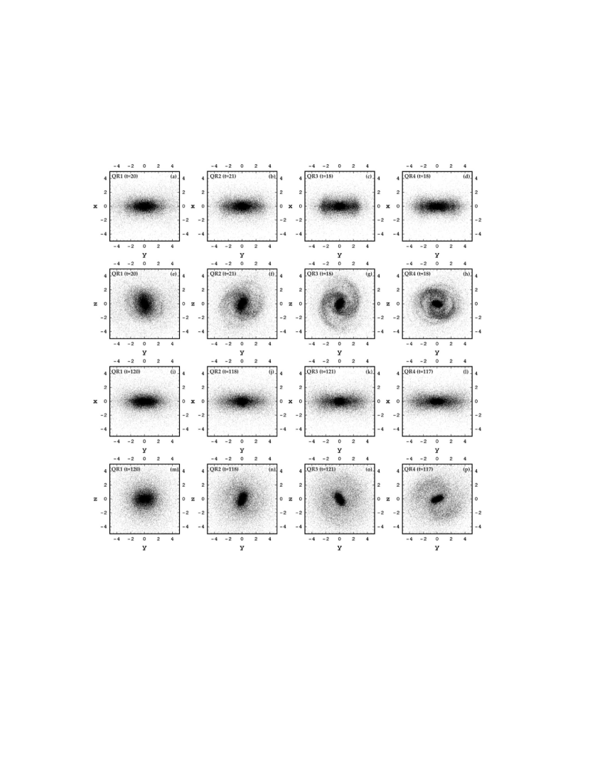
Figure 1: First row: Edge-on projections of the rotating models at $t_{1}=20,21,18,18$. Second row: Face-on projection at the same snapshots as in the first row. Density waves form a rotating bar embedded in a thick disc. The size of the bar decreases with increasing angular momentum along the sequence of the models. Spiral arms are excited on the disc that are more clearly-sighted in the models QR2, QR3, QR4. Third row: As in the first row but at a time about 100$T_{hmct}$ later. The total number of rotations from $t=0\rightarrow t\approx 120$ is 9, 11, 13, 15 for the four models respectively. An expansion on the plane of the disc has occurred, increasing along the sequence of the models. Fourth row: Face-on projections of the same snapshots as in the third row. In QR4 spiral arms are still well discernible. In QR2, QR3 they are fainter, and in QR1 cannot be seen in this projection (see Section 3.5). As it is shown in Section 5 (Fig. 16, Fig. 17) these spiral arms are almost completely formed by chaotic orbits.

In the first row of Fig. 1 the edge-on projections (y-x plane) of the four models (QR1, QR2, QR3, QR4) are shown, respectively, at their snapshots at time $t_{1}\approx 20$ of their run time. (More precisely, $t_{1}$ is $20,~{}~{}21,~{}~{}18,~{}~{}18$ for the four models, respectively. Hereafter, these times are referred simply as $t_{1}\approx 20$).

In the second row of Fig. 1 the face-on projections (on the equatorial plane, y-z) of these models are shown at the same snapshots as in the first row. In these figures we can see that the size of the bar decreases with increasing angular momentum along the sequence of the models. We can also see that density waves form two symmetric spiral arms emanating from the ends of the bar, that become more prominent along the sequence QR1, QR2, QR3, QR4.

The third and the forth row in Fig. 1 are similar to the first two rows, respectively, but at a time of about $100T_{hmct}$ later. During this long interval of time ($t=0\rightarrow t\approx 120$) the bar has described a total number of about 9, 11, 13, 15 rotations, respectively in the four models. We see that in QR4 spiral arms are still well discernible at this time. In QR2 and QR3 they are fainter. In QR1 they cannot be seen in this projection. Furthermore, we see that the distribution of mass in QR2, QR3, QR4 has been expanded along the equatorial plane by a factor that is more prominent in the QR4 model.

3.2 Radial profiles of the surface density

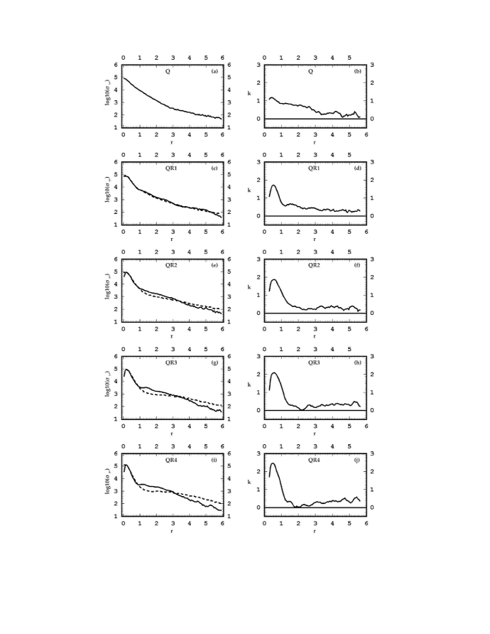
Figure 2: Left column: Radial profiles of the mean surface density $\overline{\sigma}_{yz}(r)$ for all the models at $t_{1}\approx 20$ (solid line) and at $t_{2}=300$ (dashed line). At small radii $r\lesssim 1$ the profiles become steeper and steeper along the sequence of the models. At larger radii the profiles in the rotating models become exponential. The exponential profiles show a slow time evolution tending to be flatter. (Solid line is at $t_{1}\thickapprox 20$, while dashed line is at $t_{2}=300$). Right column: The slope $k$ of the profiles as a function of the radius at $t=150$. In Q this slope decreases gradually (on the average) along the radius. In the rotating models $k$ has a pronounced maximum at $r<1$, but falls to a smaller roughly constant value at larger radii.

In the five frames of the left column of Fig. 2 the radial profiles of the mean surface density $\overline{\sigma}_{yz}(r)$ at a radius $r$ on the equatorial plane of all the models (Q, QR1, QR2, QR3, QR4) are shown as functions of the radius $r$, in $r$-$\log_{10}{\overline{\sigma}_{yz}}(r)$ scale.

As the rotation increases along the sequence of the models, the radial surface density profiles at small radii ($r\lesssim 1$) become steeper. In the rotating models the slope in the outer parts remains remarkably constant along the radius, indicating an exponential radial profile of the surface density.

The time variations of these profiles during a Hubble time are small. For example, in the frames for the models QR1,QR2,QR3,QR4, in Fig. 2 the surface density radial profiles are drawn at $t_{1}\thickapprox 20$ (solid line) and at $t_{2}=t_{Hub}=300$ (dashed line). There is a tendency of these profiles to become flatter in time. This tendency increases along the sequence of the models and it is due to a slow expansion of the mass at large radii combined with a slow contraction at smaller radii.

The exponential radial profiles of the surface density in the rotating models can also be seen in the five frames of the right column of Fig. 2 where the corresponding slopes

$$k=-\frac{d\log_{10}\overline{\sigma}_{yz}(r)}{dr}$$ (3)

are shown as functions of $r$ at an intermediate snapshot of $t=150$. We see that the value of the slope $k$ in the non-rotating Q model decreases almost constantly up to large radii. However, in the rotating models QR1, QR2, QR3, QR4 the values of $k$ show a maximum at a small radius ($r<1$), but beyond this radius, $k$ flattens and remains remarkably constant up to large radii, expressing the exponential character of the profile. Such radial profiles of the surface density are similar to the observed profiles of the discs (see, for example, Grosbol & Patsis 1998, figs.1a-c therein).

3.3 Rotation curves and angular momentum transference

It is interesting to examine the time evolution of the rotational velocity curves and the distribution of the angular momentum for each model.

In order to find the rotation curve at a given snapshot of such a system we define 50 successive cylindrical co-axial rings around the rotation axis (x), so that the mass inside every ring is the same for all the rings. The rotational velocity $v_{i}$ at the mean radius $r_{i}$ of the ring $i$ is evaluated from the equation

$$v_{i}={J_{i}\over r_{i}}$$ (4)

where

$$J_{i}=\frac{1}{N_{i}}\sum_{j=1}^{N_{i}}(y_{j}\dot{z_{j}}-\dot{y_{j}}z_{j})$$ (5)

is the mean angular momentum per particle along the x axis of the $N_{i}$ particles in the ring $i$.

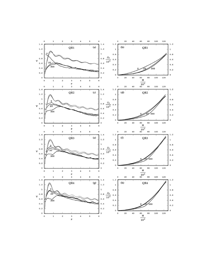
Figure 3: Left column: Rotational velocity curves. Solid lines give the rotational velocity $v_{i}(r_{i})$ evaluated from the mean angular momentum per particle in successive cylindrical rings at times $t=0,20,300$ as indicated by the numbers in the figures. These curves show that $v_{i}(r_{i})$ decreases in time particularly in the inner parts, due to the transference of angular momentum outwards. The dashed lines give the “dynamical” rotational velocity curves evaluated from the monopole terms of the potential at $t_{1}\approx 20$ and $t_{2}=300$. These curves show a small variation during this period, due to a slow redistribution of mass. Right column: The cumulative angular momentum vs the cumulative mass from the center at the same times as in the left column. At later times more mass is required in order to collect the same amount of angular momentum, as a result of the transference of the angular momentum outwards.

In the left column of Fig. 3 the rotational velocity curves of the four models are shown. In these figures the velocity $v$ is measured in units of $R_{h}/T_{hmct}$. The conversion factor in real units is

$$v_{realunits}=v*21.5{\text{km}\over\text{sec Kpc}}R_{h}$$ (6)

The value of $R_{h}$ in Kpc depends on the cosmological model, on the total mass of the system and on the value of the redshift $z_{v}$ at the epoch of virialization of the galaxy. It is given by

$$R_{h}\approx 8\text{Kpc}(\Omega h^{2})^{-1/3}{9\over 1+z_{v}}({M\over M_{12}})^{1/3},$$ (7)

where $\Omega$ is the total density parameter of the Universe, $h$ is the Hubble constant in units of $100{\text{Km}\over\text{sec Mpc}}$, $M$ is the mass of the galaxy and $M_{12}=10^{12}M_{\odot}$. For $\Omega=1$, $h=0.72$, $M=5*10^{11}M_{\odot}$ and a redshift of formation $z_{v}=5$ we get

$$R_{h}\approx 10.6\text{Kpc}$$ (8)

which is a typical value for $R_{h}$.

The solid lines in Fig. 3 give the rotational velocity curves $v_{i}(r_{i})$ evaluated from (4) at different times, namely $t=0,~{}20,~{}300$, as indicated by the numbers next to the curves.

For comparison, dashed lines in these figures give the “dynamical” rotational velocity $v(r)=\sqrt{r\dfrac{dV(r)}{dr}}$ curves as evaluated at $t_{1}\approx 20$ and at $t_{2}\approx 300$ from the centrifugal equilibrium under the forces $\dfrac{dV(r)}{dr}$ due to the monopole terms of the potential. At the end of a Hubble time the values of $v(r)$ become slightly larger near the center, while they become slightly smaller at large radii, indicating a slow redistribution of the mass during this time.

However, this variability of $v(r)$ is small compared to the evolution of the rotational velocity curves $v_{i}(r_{i})$ in all the models. In the inner parts (e.g. for $r\lesssim 1$) the rotational velocity $v_{i}(r_{i})$ becomes gradually smaller. This occurs at a decreasing rate and it is a result due to the transference of angular momentum outwards.

The transference of angular momentum outwards can be seen in the right column of Fig. 3, where the cumulative angular momentum is plotted as a function of the cumulative mass from the center at the same snapshots as the rotation curves in the left column of Fig. 3. We see that at later times more mass is required in order to collect the same amount of angular momentum. It is remarkable that the transference of angular momentum outwards depends also on the model. For example, in QR1 the distribution of angular momentum at $t_{1}=20$ is close to the distribution at $t_{2}=300$, while in QR2, QR3 and QR4 the distribution of angular momentum at $t_{1}=20$ is close to the distribution at $t=0$.

3.4 Evolution of the pattern speeds and the corotation radii

A direct consequence of the angular momentum transference is that the bar grows and its rotation slows down. We examine the deceleration of the bar, i.e. the evolution of its pattern speed and the corresponding corotation radius.

We find first, numerically, the function of time $\Phi(t)$, that gives the angle $\Phi$ of the orientation of the longest axis of the inertia ellipsoid of the mass inside a radius $r$ (containing the bar), with respect to the initial orientation of this axis. The pattern speed of the bar as a function of time is evaluated from the slope of $\Phi(t)$ at time $t$, i.e. $\Omega_{p}(t)=\dfrac{\Delta\Phi(t)}{\Delta t}$.

The corotation radius at a particular snapshot can be estimated by locating the unstable Lagrangian point $L_{1}$ from the autonomous Hamiltonian (Jacobi integral)

$$H=\frac{\dot{r}^{2}}{2}+\frac{P_{\phi}^{2}}{2r^{2}}-\Omega_{p}P_{\phi}+\frac{\dot{x}^{2}}{2}+V(\sqrt{r^{2}+x^{2}})+V_{1}(r,\phi,x)$$ (9)

where $(r,\phi)$ are the polar coordinates on the equatorial plane (yz) and $\Omega_{p}$ is the value of the pattern speed of the bar at this snapshot. In this expression the term $V(\sqrt{r^{2}+x^{2}})$ is the monopole component of the self-consistent potential at this snapshot.

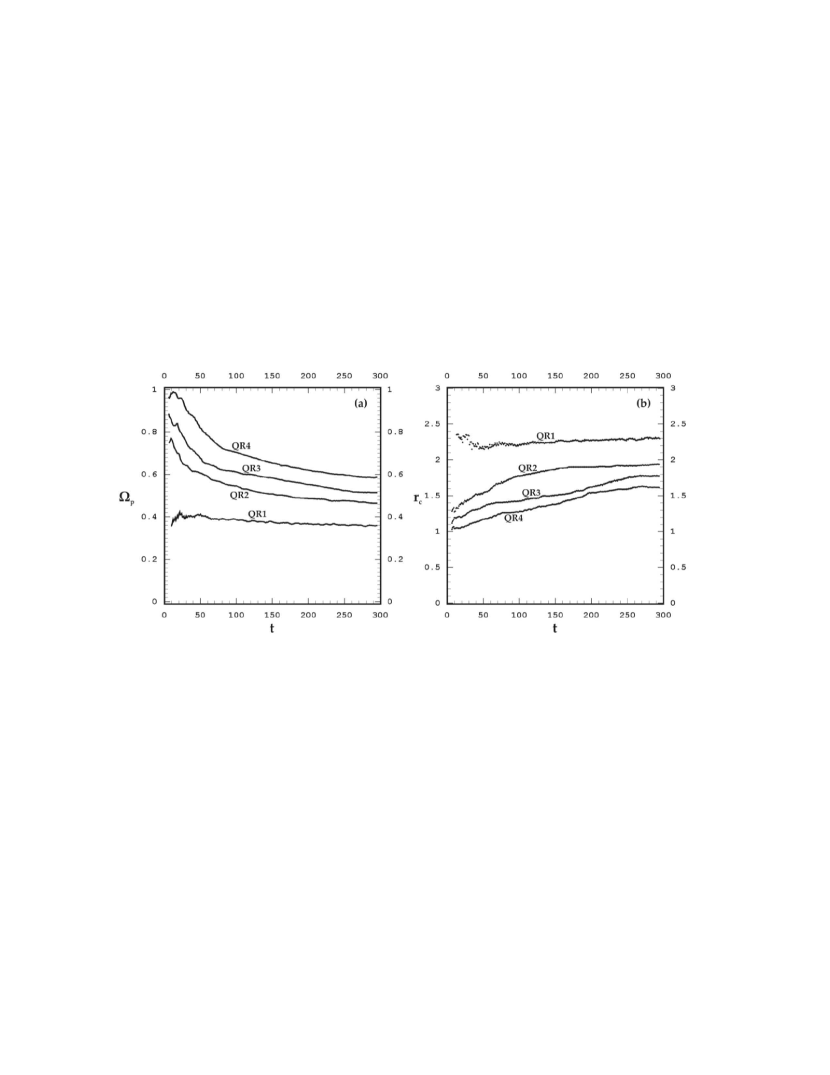
Figure 4: (a) Time evolution of the pattern speed $\Omega_{p}$ of the bar in every model. (b) Time evolution of the corotation radius $r_{c}$ (radius of the unstable Lagrangian point L1). In QR1 the pattern speed and the corotation radius remain roughly constant. In QR2, QR3, QR4 $\Omega_{p}$ decreases to about 60% the initial value, while the corotation radius increase to about 150% the initial value.

In Fig. 4 the time evolution of $\Omega_{p}(t)$ (Fig. 4a) and of the corresponding corotation radius $r_{c}$ (the radius of the unstable Lagrangian point $L_{1}$, Fig. 4b) are plotted for every model.

In QR1 $\Omega_{p}(t)$ does not vary considerably preserving a value about $0.4$ (in units of $rads/T_{hmct}$). The corotation radius also remains roughly constant at about 2.3.

In QR2, QR3, QR4 $\Omega_{p}(t)$ starts from larger values about 0.75, 0.90, and 1.0, respectively, and decreases initially faster, but more slowly later on. The corotation radii start from the values about 1.3, 1.2, 1.0 and increase by about $50\%$ at the end of the Hubble time. Gadotti & de Souza (2005, 2006) investigated the kinematics, the lengths, and the colors and ages in a good number of face-on bars in real galaxies. They classified the bars in these galaxies in old and young bars. One of their main results is that bars can survive for a Hubble time. Furthermore, the mean linear size of the young bars is $5.4\pm 1.6\text{Kpc}$, while the mean linear size of the old bars is $7.5\pm 1.2\text{Kpc}$, i.e. old bars are by about $40\%$ longer than the young bars. Thus our results are in agreement with observations, as regards the time evolution of the linear sizes of the bars.

3.5 On the longevity of spiral arms

The surface density $\sigma_{yz}(r,\phi,t)$ of the mass projected on the equatorial plane is a function of the position $(r,\phi)$ on this plane and of the time $t$. An important question regards the evolution and the longevity of the spiral pattern. In order to investigate this question we define the relative surface density fluctuation of $\sigma_{yz}(r,\phi,t)$ with respect to the mean surface density $\overline{\sigma}_{yz}(r,t)$ at the radius $r$, i.e.

$$\delta(r,\phi,t)=\frac{\sigma_{yz}(r,\phi,t)-\overline{\sigma}_{yz}\,(r,t)}{\overline{\sigma}_{yz}\,(r,t)}$$ (10)

and we analyzed $\delta(r,\phi,t)$ in Fourier component as

$$\delta(r,\phi,t)=\sum_{m}A_{m}(r,t)\cos{m[\phi-\phi_{m}(r,t)]}$$ (11)

The appearance of two spiral arms requires a serious relative contribution of the $m=2$ mode (with respect to the total power of $\delta(r,\phi,t))$ and a monotonic (on the average, increasing or decreasing) function of $\phi_{2}(r,t)$ with $r$, at least beyond a certain (not very large) radius.

The relative contribution of the $m=2$ mode is measured by

$$a_{2}^{2}(r,t)=\frac{A_{2}^{2}}{C^{2}}$$ (12)

where

$$C^{2}=\sum_{m}A_{m}^{2}$$ (13)

We define 80 successive cylindrical co-axial rings around the rotation axis (x), extended up to $r=5$, with equal width $\Delta r$. We calculate the values of $a_{2}^{2}(r,t)$ and the corresponding azimuthal angle $\phi_{2}(r,t)$ at any given time $t$.

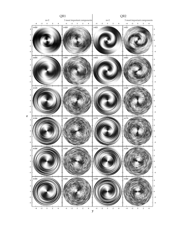
Figure 5: Two columns are plotted for every rotating model. For each model the left column gives six snapshots of the distribution on the equatorial plane $(r,\phi))$ of the function $\delta_{2}(r,\phi,t)$, i.e. the mode $m=2$ of the fluctuations of the surface density. This mode forms a spiral pattern starting slightly inside the corotation radius and going out beyond the corotation to large radii in all these snapshots. The right column gives the corresponding distributions of $\delta_{3imp}(r,\phi,t)$, resulting from the superposition of the three most important modes of the spectrum. The $m=2$ mode is obscured to some extent by other modes, but it can be discernible in the distributions of $\delta_{3imp}(r,\phi,t)$ even at the latest snapshots of the simulation, as in the bottom row in this figure.

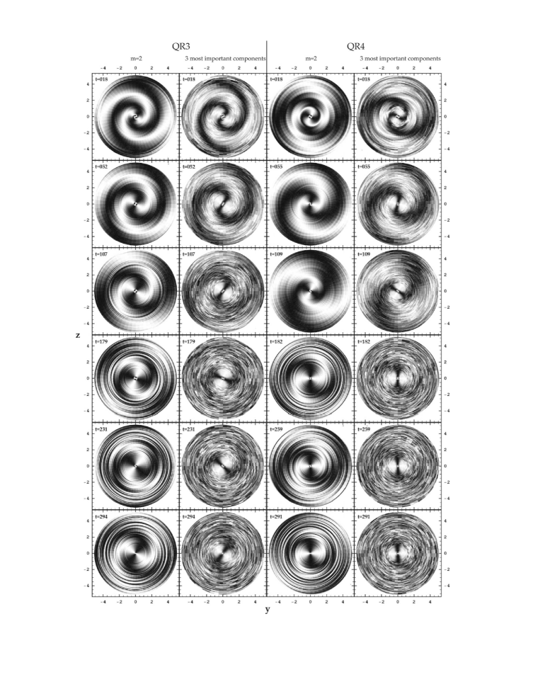
Figure 5: (Continued).

A series of 6 snapshots are displayed in Fig. 5 for every model QR1, QR2, QR3, QR4 at various times along the evolution for a Hubble time. For every model two columns are displayed. The left column shows the distribution of values of

$$\delta_{2}(r,\phi,t)=A_{2}(r,t)\cos{2[\phi-\phi_{2}(r,t)]}$$ (14)

on the equatorial plane $(r,\phi)$. In these figures black means positive and white means negative values of $\delta_{2}(r,\phi,t)$. We see that the $m=2$ mode forms a pattern composed of two parts.

The first part is a ‘bow tie’ pattern around the center, where the phase $\phi_{2}$ is independent of $r$ and corresponds to the central part of the bar, composed mainly of regular orbits (see Section 4). This ‘bow tie’ pattern ends at a radius shorter than the corotation radius, close to the Inner Lindblad resonance (ILR).

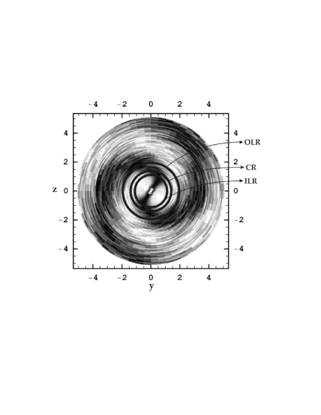
Figure 6: A magnification the distribution of $\delta_{2}(r,\phi,t)$ at the snapshot of QR4 at $t=55$ (second row, seventh column of Fig. 5), where the three cycles at the radii of the resonances ILR, CR, OLR are drawn.

An example of how the three resonances (ILR, CR, OLR) are located in the distribution of $\delta_{2}(r,\phi,t)$ is given in Fig. 6. The snapshot of QR4 at $t=55$ (second row, seventh column of Fig. 5) is shown in magnification in Fig. 6, with three cycles drawn at the radii of the above resonances.

The second part in the distribution of $\delta_{2}(r,\phi,t)$ is a two-armed spiral pattern emanating from the ends of the bar near the corotation radius. This structure appears in all the models and, despite its intermittent behavior described below, it is recreated up to the end of the Hubble time for all the models. Notice that, during the Hubble time the bar has described about 19, 25, 29 and 33 rotations in the four models QR1, QR2, QR3, QR4, respectively.

The right column for each model in Fig. 5 gives the distribution of $\delta_{3imp}(r,\phi,t)$ on the equatorial plane, as it comes out from the superposition of the three most important modes (i.e. the modes with the three highest amplitudes) of the spectrum at the same snapshots as the left column. Most frequently and for the majority of the rings outside the corotation radius, three most important modes are those with $m=2,4,6$. Sporadically at various rings and occasionally in time the modes with $m=3,5,8,10,12$ appear also in $\delta_{3imp}(r,\phi,t)$.

A careful examination of the figures in the right column of each model in Fig. 5 shows that, although the distribution of the $m=2$ mode is to some extent obscured by the other modes, it is still discernible even at the latest snapshots (see for example the last row in Fig. 5, where the snapshots at $t=288,~{}~{}280,~{}~{}294,~{}~{}291$ for the four models are displayed).

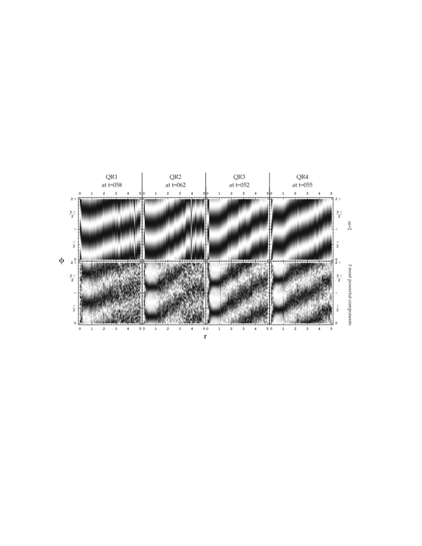
Figure 7: First row: Distributions of $\delta_{2}(r,\phi,t)$ on a rectangular frame $(r,\phi)$ for the four models at the snapshots of the second row of Fig. 5. Beyond the corotation radius the phase $\phi_{2}(r,t)$ is (on the average) a monotonic almost linear function of $r$, revealing a spiral pattern. Second row: As in the first row, but for $\delta_{3imp}(r,\phi,t)$. The obscuration of $\phi_{2}(r,t)$ by the other modes is rather small.

As regards the dependence of the azimuthal phase $\phi_{2}(r,t)$ on the radius $r$ along the spiral arms this is very close to linear, on the average. This can be seen if we plot the distributions of $\delta_{2}(r,\phi,t)$ and $\delta_{3imp}(r,\phi,t)$ on a rectangular frame $(r,\phi)$ as shown in Fig. 7 for the snapshots of the four models shown in the second row of Fig. 5, for example. The spiral arms are displayed in this figure by dark lanes along almost straight oblique lines beyond the corotation radius up to a radius $r=5$, indicating that $\phi_{2}(r,t)$ is approximately linear in $r$ along the spiral arms.

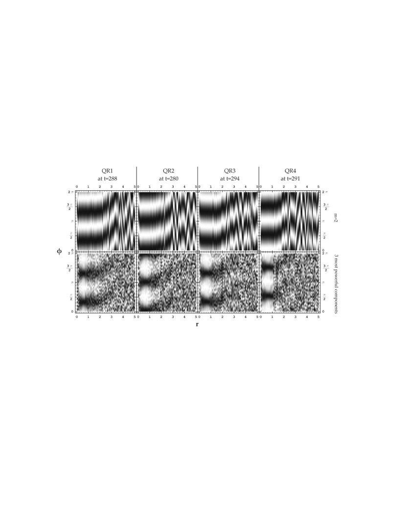
Figure 8: As in the first and the second row of Fig. 7, but for the snapshots of the last row in Fig. 5. In the first row the dark lanes are along a straight line segment between the corotation radius and $r\approx 3$ or $3.5$. In the second row, despite the obscuration by other modes at this late snapshot, the spiral structure of the $m=2$ mode is still discernible.

Fig. 8 is the same as Fig. 7, but for the latest snapshots of the four models shown in the last row of Fig. 5. In these late snapshots of evolution the linear dependence of $\phi_{2}(r,t)$ on $r$ is shorter, extended from the corotation radii to a radius of about $r=3$ or $3.5$.

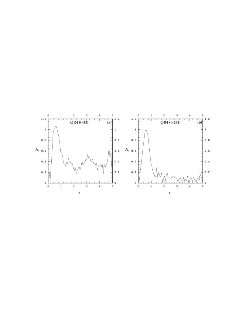
Figure 9: The size of the amplitude $A_{2}(r,t)$ of the $m=2$ mode (eq. 14) as a function of the radius $r$ at the two snapshots of QR4 shown in the second and the sixth row of Fig. 5.

In order to have some idea of the absolute size of the $m=2$ mode at the early and the late stages of evolution, we examine the amplitude $A_{2}(r,t)$ of $\delta_{2}(r,\phi,t)$ in (14). As an example, in Fig. 9 we give $A_{2}(r,t)$ as a function of $r$ at the two snapshots of QR4 shown in the second row ($t=55$) and the last row ($t=291$) of Fig. 5. In Fig. 9a (snapshot at $t=55$) the amplitude $A_{2}(r,t)$ has a maximum value about 1.1 inside the bar ($r<1$) and falls to a level of about 0.4 in the region of spiral arms. In Fig. 9b ($t=291$) the maximum value of $A_{2}(r,t)$ in the bar is only slightly reduced. In the region of spiral arms, however, it falls to the level of about 0.1 or 0.2.

Ohta, Hamabe & Wakamatsu (1990) estimated the relative amplitude $I_{2}(r)/I_{0}(r)$ of the $m=2$ of the light distribution along the radius in real barred-spiral galaxies. Similar estimations of $I_{2}(r)/I_{0}(r)$ are given by Buta, Block & Knapen (2003) and by Buta et al. (2005) for different samples. Under the assumption of constant mass-to-light ratio along the radius of a galaxy, the quantities $I_{2}/I_{0}$ and $A_{2}(r,t)$ are the same. In the region of spiral arms the values of $A_{2}(r,t)$ given above are in quite good agreement with the values of $I_{2}/I_{0}$ found in real galaxies by the above authors. The same is true for the four models.

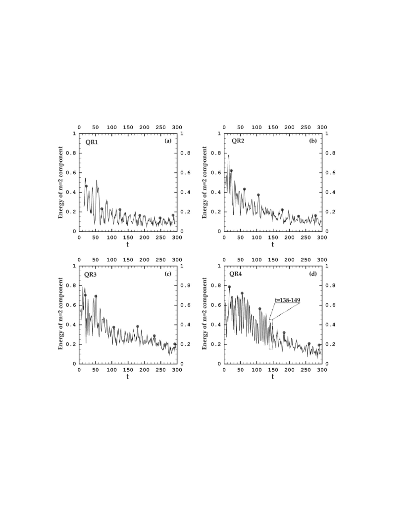
Figure 10: Evolution of the mean relative power of the $m=2$ mode $<a_{2}^{2}>(t)$ evaluated in the region with radii between the corotation radius $r_{c}$ and $r_{c}+1$. This quantity oscillates quasi-periodically in a time scale depending on the rotation period of the bar and decreases on the average due to the growth of noise and the higher Fourier modes. The dots on the top of six peak corresponds to the six snapshots shown in Fig. 5. In (d), the box with dashed line sides gives the time window of the snapshots of Fig. 11.

In order to estimate the time evolution of the relative contribution of the $m=2$ mode in the whole power spectrum of $\delta(r,\phi,t)$ we define the mean value $<a_{2}^{2}>(t)$ of $a_{2}^{2}(r,t)$ from all the rings with radii between the corotation radius $r_{c}$ and $r_{c}+1$. In Fig. 10 the quantity $<a_{2}^{2}>(t)$ is plotted as a function of time for all the rotating models. We see that $<a_{2}^{2}>(t)$ oscillates up and down, but on the average it decays with time, tending to a minimum value somehow smaller than 0.2 at $t_{2}=300$. It is remarkable that the mean values of $<a_{2}^{2}>(t)$ at early times (e.g. at $t_{1}\approx 20$), as well as the time intervals when $<a_{2}^{2}>(t)$ maintains values greater than a certain value, e.g. $0.3$, increase along the sequence of the models.

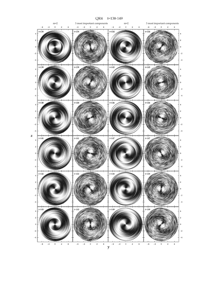
Figure 11: Detailed snapshots (every $\Delta t=1T_{hmct}$) of $\delta_{2}(r,\phi,t)$ and $\delta_{3imp}(r,\phi,t)$ (in pairs as in Fig. 5) for the model QR4, during the $18^{th}$-$19^{th}$ period of rotation of the bar. Observing carefully the evolution of $\delta_{2}(r,\phi,t)$, we see that a continuous spiral arm is formed at $t=143$ (first column, last row) out to radii more than $r=4$. At this time $<a_{2}^{2}>(t)$ has a maximum in Fig. 10d (inside the box with dashed lines). At the next snapshots $t=144\longrightarrow 147$ (third column) the bar goes temporarily out of phase with respect to the previously excited wave, which travels outwards and rotates more slowly than the bar. The continuation of the spiral arms is temporarily broken. The bar emits new waves travelling outwards that come in phase with the previous wave at $t=149$ and form again a continuous spiral wave extending out to large radii. This process is repeated up to the end of the Hubble time, although spiral arms become fainter at very late snapshots. The $m=2$ mode is discernible also in the projections of $\delta_{3imp}(r,\phi,t)$ at the same snapshots (second and fourth columns).

Notice that the bold dots drawn on the top of six of the peaks in Fig. 10 indicate the snapshots displayed in Fig. 5. An example of the evolution between two successive peaks is described below in Fig. 11.

The oscillations of $<a_{2}^{2}>(t)$ in Fig. 10 show a periodicity related to the period of rotation of the bar. This effect certainly betrays information related to the mechanism of excitation and propagation of spiral waves. It requires a much thorough investigation, but here, we will give a short qualitative description of what seems to happen, based only on the observation of a number of successive snapshots. In order to see this effect in more details, we select a series of 12 successive snapshots (at every $\Delta t=1T_{hmct}$) in the time interval between $t=138$ and $t=149$ of the evolution of the QR4 model during the 18th-19th rotation of the bar. This interval of time is marked by a box with dotted lines in Fig. 10d. During this interval the quantity $<a_{2}^{2}>(t)$ describes about 1.5 oscillations, i.e. minimum-maximum-minimum-maximum.

In Fig. 11 the distributions of $\delta_{2}(r,\phi,t)$ and $\delta_{3imp}(r,\phi,t)$ are shown (in pairs as in Fig. 5) for the 12 successive snapshots ($t=138\rightarrow 149$). Observing carefully these distributions we can describe the following mechanism:

Spiral pattern is due to a wave fluctuation mode of $m=2$ on the surface density, that is excited by the bar. This wave travels outwards and rotates more slowly than the bar. The bar goes out of phase with respect to a previously excited part of the mode. Two parts of this mode, excited at a small difference of time are not always in phase. In this case the continuation of the spiral shape of the wave can be interrupted. The quantity $<a_{2}^{2}>(t)$ has a minimum. The two parts of this mode come in phase quasi-periodically producing a global spiral wave with maximum amplitude $<a_{2}^{2}>(t)$ and smoothly joined azimuthal phases. They come out of phase again and the global spiral structure is temporarily deformed, or interrupted and so on.

It is possible in this case that, temporarily, Quarter-Turn Spirals (QTS) appear as, for example, in the snapshot at $t=147$ (Fig. 11). Notice that QTS are observed e.g. in NGC 3631 and NGC 1365, (Fridman, Khoruzhii & Polyachenko 2002; Polyachenko & Polyachenko 2002; Polyachenko, 2002a, 2002b).

It is also possible that spiral arms can be so confused, due to an irregular dependence of $\phi_{2}(r,t)$ on $r$ that can hardly be discernible, but the dependence of $\phi_{2}(r,t)$ on $r$ becomes smooth again and continuous spiral arms are re-created again in about half the period of the bar, or in any case in less than a period of rotation of the bar. This process is repeated all during the Hubble time in our experiments, when the bar describes a good number of rotations ranging from 19 rotations in QR1 to 33 rotations in QR4, although the relative power of the $m=2$ mode with respect to higher modes decreases by a factor of about 2 or 3.

3.6 Secular evolution and the mass in chaotic motion

In general the fraction of mass in chaotic motion, the spatial distribution of this mass, the mean level of the Lyapunov numbers and their distribution among the chaotic orbits are important parameters related to the morphology and the secular evolution of galaxies.

If chaotic orbits have so small Lyapunov numbers that the rate of their chaotic diffusion in a Hubble time cannot be efficient, or if chaotic orbits are only a small fraction of the total mass, or if they are uniformly distributed inside the equipotential surface of their energy, they cannot drive any secular evolution in a galaxy.

Secular evolution can be driven within a Hubble time by chaotic orbits provided that:

i) Lyapunov times of chaotic orbits do not exceed the Hubble time

ii) the mass in chaotic orbits with such Lyapunov times is a good fraction of the total mass and

iii)these chaotic orbits occupy a limited part of their available phase space.

A better understanding of the various features of our models can be obtained, if we make a distinction between regular and chaotic orbits. The method of the distinction and the results obtained are discussed in the next section.

4 Mass in chaotic versus mass in regular motion

We use the method introduced in Voglis et al. (2002) to find the fraction of mass in chaotic motion at various snapshots of our models and compare the results.

As a measure of the chaotic character of an orbit one can use the mean logarithmic divergence between neighboring orbits in a finite time, called Finite Time Lyapunov Characteristic Number ($FT-LCN$) defined by

$$FT-LCN=\frac{1}{t}\log{\frac{\xi(t)}{\xi(0)}}$$ (15)

where $\xi(t)$ is the length at time $t$ of the deviation vector from an orbit under study and $\xi(0)$ is its initial value.

The deviation vector $\vec{\xi}(t)$ is defined in the 6-dimensional phase space $\vec{\xi}(t)=(dx,dy,dz,dp_{x},dp_{y},,dp_{z})$ from the differentials of the position and momentum variables $(x,y,z,p_{x},p_{y},p_{z})$. It is evaluated from the variational equations, derived by differentiating the equations of motion. The coefficients of the variational equations are evaluated from the solutions of the canonical equations of motion resulting from the Hamiltonian (9), when this Hamiltonian is applied to a particular snapshot of the self-consistent run of our systems.

As it is well known (see e.g. Contopoulos 2004, for a review) the maximal Lyapunov Characteristic Number $LCN$ of an orbit is the limit of $FT-LCN$ as $t$ tends to infinity. If $LCN$ is zero the orbit is regular (called also ordered), while if $LCN$ acquires a positive constant value the orbit is chaotic and the constant value of the $LCN$ is a measure of the chaotic character of the orbit.

Since in practice the orbit can be integrated only for a finite time $t_{max}$, $LCN$ can only be approximated by the values of $FT-LCN$. However, the values of $FT-LCN$ never become exactly zero. In regular orbits the values of $FT-LCN$ tend to zero on the average as $\log{t}/t$ (with an average slope $1/t$). In chaotic orbits, for a transient period $t_{L}$, the values of $FT-LCN$ again decrease on the average following the same law ($\log{t}/t$), but later on they tend to be stabilized at a constant value $L$. This value can be considered as an estimate of the $LCN$ of the orbit.

If $t_{L}$ is known, a first estimate of $L$ is $L\approx\log{t_{L}}/t_{L}>1/t_{L}$. Thus the detectable values of $LCN=L$ of a chaotic orbit are limited by the inequality $L>1/t_{max}$. In order to obtain a distinction between chaotic and regular orbits in terms of $L$, it is necessary to define a threshold value of $L=L_{min}\gtrsim 1/t_{max}$. All the orbits for which $FT-LCN$ has already been stabilized at a value $L>L_{min}$, at $t=t_{max}$, can be characterized as chaotic. The maximum Lyapunov time of these orbits is $T_{L,max}=1/L_{min}$. For insuring that all the orbits, that practically behave as chaotic, have been detected, $T_{L,max}$ should be remarkably larger than a Hubble time.

On the other hand, the orbits for which $FT-LCN$ at $t=t_{max}$ still decreases on the average as $\log{t}/t$ could be either regular (with $LCN=0$), or chaotic but with $LCN<L_{min}$. All these orbits can conventionally be characterized as regular orbits.

A difficulty arising in applying this method in galaxies is the fact that in galaxies there are orbits evolving in very different characteristic time scales. The radial period $T_{rj}$ (i.e. the time for a orbit to go from its apocenter to pericenter and back to apocenter) of the orbit $j$ depends on the binding energy $E_{j}$ of this orbit according to the relation $T_{rj}\sim\mid E_{j}\mid^{-3/2}$, almost independently of the angular momentum of the orbit. This relation is exact in a Keplerian field, as well as in the isochrone potential model. In gravitational N-body simulations, the same relation still holds with a remarkable accuracy (Voglis, 1994).

In galaxies the binding energies of individual orbits, and therefore the corresponding radial periods, spread to more than four orders of magnitude. The departure from integrability of an orbit depends on the variability per dynamical time of the actions associated with the orbit. If in an orbit a certain variation of actions takes place in 1 dynamical time and in another orbit the same variation takes place in 10 dynamical times, the departure from integrability is larger in the former case.

Therefore, a fair estimate of the departure of orbits from integrability can be obtained by integrating the orbits for the same number $N_{r,max}$ of radial periods than for the same time $t_{max}$.

For this reason we use the Specific Finite Time Lyapunov Characteristic Number ($SFT-LCN$) denoted by $L_{j}$ for every orbit $j$. The term ‘Specific’ is used to declare that $L_{j}$ is evaluated in units of the inverse radial period $1/T_{rj}$ of the particular orbit. This makes the values of $L_{j}$ almost invariant in the characteristic time scale of the orbit. A particular threshold value of $L_{j}=L_{min}$ is a better index for distinction between regular and chaotic orbits.

A disadvantage of the index $L_{j}$ is that the Lyapunov times measured by $T_{L}=T_{rj}/L_{j}$ (in fixed time units) are different for orbits with the same $L_{j}$, but different energies. The chaotic diffusion of an orbit is important for times greater than its Lyapunov time $T_{L}$. Among the chaotic orbits, only those with $T_{L}<t_{Hub}$ are able to develop effective chaotic diffusion in a Hubble time.

In order to estimate the ability of orbits for an effective chaotic diffusion in a Hubble time we use, instead of the index $L_{j}$, the index

$$L_{cu}=L_{j}\frac{T_{hmr}}{T_{rj}},$$ (16)

which is the value of $FT-LCN$ measured in a common unit $1/T_{hmr}$ for all the orbits, where $T_{hmr}$ is the radial period of an orbit with binding energy $E_{hmr}$. A Hubble time is $t_{Hub}=300T_{hmct}=100T_{hmr}$, as described in the introduction. The Lyapunov times of the orbits in common units of $T_{hmr}$ are $T_{L}=1/L_{cu}$. Therefore, chaotic diffusion of an orbit $j$ becomes important in a Hubble time, if $T_{L}\lesssim t_{Hub}$, or if $L_{cu}\gtrsim 10^{-2}$.

An alternative index that can be combined with the index $L_{j}$ for the distinction between regular and chaotic orbits is the so called Alignment Index ($AI$) defined as

$$AI=\sqrt{1-\left|\frac{\vec{\xi}_{1}(t)\centerdot\vec{\xi}_{2}(t)}{\xi_{1}(t)\xi_{2}(t)}\right|}$$ (17)

where $\vec{\xi}_{1}(t)$ and $\vec{\xi}_{2}(t)$ are two different deviation vectors of the same orbit. This index is a direct measure of the angle between the two deviation vectors.

The behavior of the deviation vectors in four-dimensional symplectic maps or in three-dimensional Hamiltonian systems has been examined in Voglis, Contopoulos & Efthymiopoulos (1998,1999) and Voglis et al. (2002). In the case of ordered motion, two initially arbitrary deviation vectors, after a transient period of time, become tangent to the surface of the corresponding torus. On the surface of the torus they oscillate around each other. Thus, the angle between the two vectors (and hence the alignment index $AI$) shows no systematic variation, but remains always around a finite mean value.

On the contrary, if the orbit is chaotic, the directions of the two deviation vectors tend exponentially to coincide to each other along the same direction (parallel or antiparallel), which is the direction of the nearby passing most unstable manifold. Thus, the index $AI$ tends exponentially to zero.

In Voglis et al. (2002) the alignment index $AI$ was defined as the smaller between the sum or the difference of the two deviation vectors (normalized to unity at every time step), depending on whether they are antiparallel or parallel, respectively. This index is often called SALI (Smaller ALignment Index, Skokos 2001). But by the definition given in (17) the distinction between parallel or antiparallel deviation vector is avoided.

The adopted maximum number of radial periods of the run time $t_{j,max}$ of the orbit $j$ is $N_{r,max}=t_{j,max}/T_{rj}=1200$ for all the orbits. The corresponding threshold value of $L_{j}$ is $L_{j}=10^{-2.8}$. By evaluating simultaneously the two indices ($AI_{j}$ and $L_{j}$) along the orbits of the system we can obtain a reliable distinction between ordered and chaotic orbits in our models at a particular snapshot of their self-consistent run.

It should be stressed that by this distinction we only check whether the positions and velocities of the particles, if they are considered as initial conditions in the fixed potential of the particular snapshot, belong to regular or to chaotic orbits. In general, the same initial conditions in a self-consistent run, i.e. in a time varying potential, do not lead exactly to the same orbits. This distinction regards a particular snapshot and informs us only about the character of the initial conditions of the orbits in the fixed potential of this snapshot. However, if the system is in a well established equilibrium (it has no significant secular evolution) the coefficients of the potential have only a small noise (less than 1%). We have shown (Voglis et al. 2002) that, in this case, if the method of distinction is applied at a different snapshot, e.g. a time of $100T_{hmct}$ later, only a small number of particles in the system (less than $3\%$) have changed the character of their motion (from regular to chaotic, or vice versa), because of the noise in the coefficients of the potential. Thus, an uncertainty in estimating the fractions of mass in regular or chaotic motion of the order of about $3\%$ always exists.

In a system that develops significant secular evolution, as it is the case of our rotating systems, or the case when the system contains a massive central concentration (e.g. Kalapotharakos et al. 2004), the coefficients of the potential can considerably vary in time, resulting in a considerable change on both the number of chaotic orbits and on the distribution of the Lyapunov numbers. Useful pieces of information about the secular evolution of such systems can be obtained by repeating the distinction between regular and chaotic orbits at several snapshots.

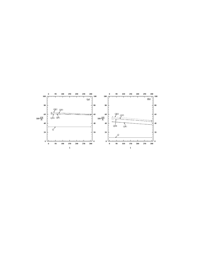
Figure 12: (a) The fraction of mass in chaotic motion detected at $t_{1}\approx 20$ and at $t_{2}=300$ for the all the models. Rotation produces a serious increase of this fraction, (by a factor of $\approx 2$, compare the non-rotating Q model with the rotating models). (b) The fraction of mass in every model, that can develop effective chaotic diffusion in a Hubble time (with Lyapunov numbers $L_{cu}>10^{-2}$). Rotation not only increases the total chaotic mass, but also produces a shift in the Lyapunov numbers, so that this fraction increases by a factor of 6 or 7 in the rotating models.

In Fig. 12a the fractions of mass detected in chaotic motion are shown by points at the snapshots of $t_{1}\approx 20$ and $t_{2}=300$ joined by lines for all the models as indicated in the figure. In the non-rotating model Q the fraction of mass in chaotic motion remains constant at about $32\%$ all along the period of a Hubble time. In the rotating models the fraction of mass in chaotic motion is at the level of about $60\%$ to $65\%$ and remains on this level, presenting only a small decrease (of a few %) at the end of the Hubble time. (Notice that all the fractions of mass in this article are with respect to the total mass of the system).

A similar representation is shown in Fig. 12b, but for the fractions of mass with $L_{cu}>10^{-2}$, that can develop chaotic diffusion in a Hubble time. These fractions range from about $45\%$ to $55\%$ at $t_{1}$ and from about $35\%$ to $45\%$ at $t_{2}$. In other words, the Lyapunov numbers $L_{cu}$ of a fraction of about $10\%$ of the total mass have been shifted to values smaller than $10^{-2}$ at $t_{2}$. This indicates a tendency of the mass to be self-organized to some degree.

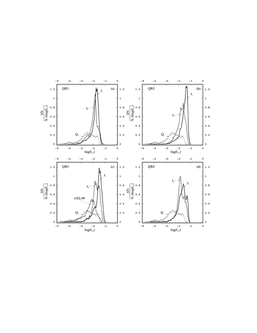
Figure 13: Distributions of the chaotic mass along the $\log L_{cu}$ axis normalized with respect to the total mass. The solid line gives this distribution at $t_{1}$, while the dashed line at $t_{2}$ for every rotating model. The dotted line with index Q corresponds to the non-rotating model. The transition from the curve Q to the curve $t_{1}$ is due to the rotation. The dotted line with index $t_{1}(\Omega_{p}=0)$ in (c) gives the chaotic mass in a hypothetical model with the same self-consistent potential as QR3, but not rotating ($\Omega_{p}=0$). The transition from the curve Q to $t_{1}(\Omega_{p}=0)$ is only due to the different geometry of the distribution of the mass caused by the rotation. The transition from the curve $t_{1}(\Omega_{p}=0)$ to the curve $t_{1}$ is due to the increase of the chaotic mass and to the shift of the Lyapunov numbers due to the resonant effects. The transition from the curve $t_{1}$ to the curve $t_{2}$ shows a slow tendency of the system for self-organization.

The distributions of chaotic orbits along the axis of $\log{L_{cu}}$ are shown in Fig. 13 for the four rotating models. In every model the solid line comes from the snapshot at $t_{1}$ and the dashed line comes from the snapshot at $t_{2}$. The dotted line with index Q in this figure gives the distribution of the Q model, for comparison. All the distributions are normalized with respect to the total mass of the system.

At $t_{1}$ the maximum of these distributions occurs at values of $\log{L_{cu}}$ about $-1.7,-1.5,-1.5,-1.7$ for QR1, QR2, QR3, QR4, respectively, i.e. by about one order of magnitude larger than in the Q model, in which the maximum of the distribution occurs at about $-2.5$. This difference is important for the chaotic diffusion in a Hubble time. A direct consequence of this shift of the Lyapunov numbers is that the fraction of mass that can develop effective chaotic diffusion in a Hubble time ($L_{cu}>10^{-2}$) presents a considerable increase from the level of $8\%$ to the level of $45\%-55\%$, as mentioned above.

It comes out, therefore, that rotation enhances chaos, not only as regards the fraction of mass in chaotic motion, but also as regards the magnitude of the Lyapunov numbers, that are seriously shifted towards larger values. This impressive enhancement of chaos is due to the rotation.

Rotation produces two effects. A re-distribution of mass that creates a different self-consistent potential and a series of resonances that affect the dynamical evolution of the system. A reasonable question at this point is, which of the two effects is more responsible for the enhancement of chaos?

As we have seen in the models Q and C, if there is no rotation chaos increases with increasing departure from sphericity, e.g. with increasing maximum ellipticity. The new distribution of mass caused by rotation is more complicated than the distribution of mass in the non-rotating models. Namely, the whole distribution of mass is flatter, but the density becomes larger near the center. A central bar is formed surrounded by a thin and a thick disc. On the disc the surface density shows an exponential radial dependence and a spiral azimuthal dependence. This more complicated structure is expected to be in favor of chaos.

On the other hand, the rotation of the above pattern with a speed $\Omega_{p}$ introduces instabilities and a sequence of important overlapping resonances between $\Omega_{p}$ and the frequencies of orbits. Interactions between resonances is known to be an important source of chaos (Contopoulos 1966; Rosenbluth et al. 1966; Walker & Ford 1969; Chirikov, Israilev & Shepelyansky 1971; Zaslavsky & Chirikov 1972; Chirikov 1979. For a review see Contopoulos 2004).

These two effects cannot be disentangled. However, we can check to what extend each effect is responsible for chaotic motion by the following test. We consider, for example, that the distribution of mass at a given snapshot, e.g. at $t_{1}\approx 20$, of QR3 does not rotate. We run the orbits in the fixed potential of this snapshot without rotation ($\Omega_{p}=0$) and separate the mass in regular and in chaotic motion by the same method. The resulting distribution of the chaotic mass along the $\log{L_{cu}}$ axis in this case (non-rotating potential of QR3 at $t_{1}$) is shown by the dotted line with index $t_{1}(\Omega_{p}=0)$ in Fig. 13c. The corresponding fraction of mass is about 46% of the total mass, while the fraction with $\log{L_{cu}}>-2$ is only about 15%. Notice that, more than 95% of the identities of particles under the curve $t_{1}(\Omega_{p}=0)$ in Fig. 13c appear also in the group of particles under the curve $t_{1}$ of the same figure.

The enhancement of chaos between the curves Q and $t_{1}(\Omega_{p}=0)$ can be attributed to the scattering of high energy orbits by the bar and to the torques due to the spiral structure. Such torques are not negligible. (Notice that this is also true in real galaxies, see e.g. Gnedin, Goodman & Frei 1995; Kormendy & Kennicutt 2004; Block et al. 2004). Thus, we conclude that the complicated pattern itself (formed by the rotation) increases the mass in chaotic motion even under the absence of resonances.

In the rotating pattern, resonances increase further the fraction of chaotic orbits. Furthermore, instabilities introduced by the resonances and interactions between them produce a remarkable increase on the mean level of the Lyapunov numbers. (Compare the curves $t_{1}(\Omega_{p}=0)$ and $t_{1}$ in Fig. 13c).

Thus, we conclude that rotation enhances the mass in chaotic motion, as well as the mean level of the Lyapunov numbers by two collaborating mechanisms, i.e. the more complicated distribution of mass and the instabilities introduced by resonances and interactions between resonances.

During the secular evolution of the systems, part of the mass in chaotic motion is self-organized, or tends to smaller Lyapunov numbers. Comparing the distributions of the chaotic mass along the $\log{L_{cu}}$ axis at $t_{1}\simeq 20$ (solid line) and $t_{2}=300$ (dashed line) in Fig. 13, shows that the maximum is shifted towards smaller values and the mass in chaotic motion decreases. The mass with values of $\log{L_{cu}}$ above the limit of $-2$ at $t_{2}=300$ becomes by about 10% smaller as described above (Fig. 12).

A question at this point is how the self-organization observed in this investigation can be compatible with the second law of thermodynamics. What happens to the entropy?

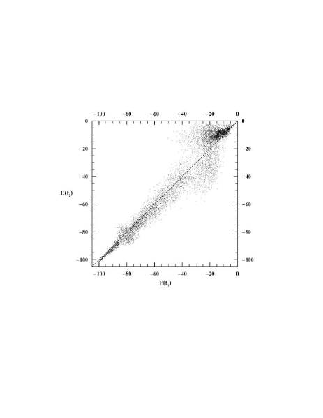
Figure 14: The binding energies of the particles $E(t_{1})$ at $t_{1}$ vs the binding energies of the particles $E(t_{2})$ at $t_{2}$ in QR4. During the evolution from $t_{1}$ to $t_{2}$ particles at lower energies lose energy, while particles at higher energies gain energy. This allows self-organization in the inner parts, although the total entropy of the system is expected to increase due to the second law of thermodynamics.

Self-gravitating systems have negative specific heat (Lynden-Bell & Wood 1968; Binney & Tremaine 1987). The angular momentum transference outwards causes an expansion of the outer material of the disc and a shrinking of the inner material. The energy is redistributed along the radius of the system. In the inner parts the energy decreases, while in the outer parts the energy increases. An example of comparison of the binding energies of individual particles from QR4 is shown in Fig. 14 ($E(t_{1})$ at $t_{1}$ and $E(t_{2})$ at $t_{2}$). Particles at lower energies lose some of their energy and are projected below the diagonal in this figure, while particles with high energies gain energy and they are projected above the diagonal. Some particles can acquire even positive energies and escape from the system, so the energy of the bound part becomes smaller. This really happens for about $0.5\%$ of the particles in each model, as already mentioned at the end of Section 2. The redistribution of energies is associated with a redistribution of entropy. Some entropy of the inner parts is transferred outwards. Thus, although the total entropy of the system is expected to increase according to the second law of thermodynamics, self-organization is possible due to the redistribution of the binding energies that allows redistribution of the entropy as well.

5 Spatial distribution of the mass in chaotic motion

The values of the Jacobi integral of the majority of regular orbits belong to the deepest parts of the potential well, while the majority of chaotic orbits have values of the Jacobi integral around the maximum value $h_{J}(r_{c})$ of the effective potential at the corotation radius $r_{c}$.

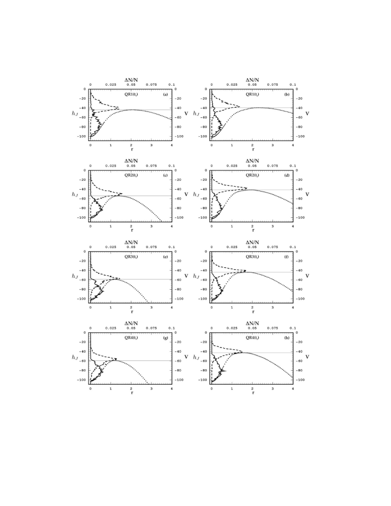
Figure 15: Distribution of the mass (upper horizontal axis) in regular motion (solid line) and in chaotic motion (dashed line) along the Jacobi integral $h_{J}$ (left vertical axis). The dotted line gives the effective potential (right vertical axis) as a function of the radius $r$ (lower horizontal axis) taken along the longest axis of the bar. The left column refers to the rotating models at $t_{1}$ and the right column at $t_{2}$. The values of the potential are normalized so that the deepest value at the center of QR1 is $-100$. Regular orbits always dominate in the inner parts of the system, well inside the corotation radius. Chaotic orbits are always concentrated near corotation. The peak of their distribution is always slightly above the Lagrangian points $L1$,$L2$.

In Fig. 15 the effective potential in the rotating frame (right vertical axes V in each panel) is given as a function of the radius $r$ (lower horizontal axis r), when $r$ is taken along the longest axis of the bar (dotted line). (The values of the potential are normalized so that the deepest value of the potential at the center of QR1 is $-100$). A horizontal straight line is also plotted at the maximum value $h_{J}(r_{c})$ of this potential.

In the same figures, for comparison, the left vertical axis gives the values of the Jacobi integral $h_{J}$ of the orbits. The upper horizontal axis gives the fraction of mass $\Delta N_{c}(h_{J})/N$ of chaotic orbits (dashed curve) and the fraction of mass in regular orbits $\Delta N_{r}(h_{J})/N$ (solid curve) as they are distributed along the $h_{J}$ axis.

The left column of Fig. 15 refers to the four models at $t_{1}$. The right column is similar to the left column, but at $t_{2}$.

As it can be seen in Fig. 15 chaotic orbits are concentrated around the maximum values $h_{J}(r_{c})$ of the effective potential (the unstable Lagrangian points $L1$, $L2$). The maximum of the distribution of chaotic orbits always occurs for energies slightly above the corotation energy $h_{J}(r_{c})$. Regular orbits dominate in the inner parts well inside the corotation radius.

The different distribution of regular and chaotic orbits along the energy axis implies an important difference in their spatial distribution.

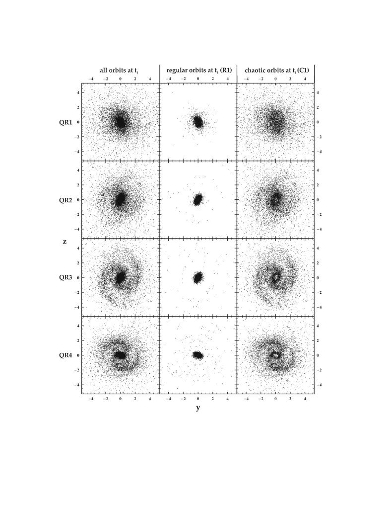
Figure 16: Projections on the equatorial plane of the four models at $t_{1}\approx 20$. Every row belongs to the same model. A sample of 1 every 12 particles uniformly distributed along the mass of the model are plotted. The middle panel in every row shows the spatial distribution of the particles in regular orbits (R1), while the right panel shows the particles in chaotic orbits (C1) of this sample. A spiral pattern (more clearly-sighted in QR2, QR3, QR4) is almost completely formed by chaotic orbits.

In Fig. 16 the projections of the rotating models on their equatorial plane are shown at $t=t_{1}$. The panels of the same row correspond to the same model at the same time. In this figure a sample of 1 particle every 12 particles, uniformly distributed along the mass of the system, is plotted in the left panel for each model.

From this sample the set of particles that are detected in chaotic motion at $t_{1}$ is denoted by C1 and is plotted separately in the right panel of the same row, while the set of the particles that are detected in regular motion at this time is denoted by R1 and is plotted separately in the middle panel.

By comparing the set R1 (middle panel) with the set C1 (right panel) in a row of these figures we infer that the spiral arms that are clearly-sighted in QR2, QR3, QR4 are almost completely formed by chaotic orbits.

This is a striking new result revealing that a mechanism able to produce spiral arms should be sought in the properties of chaotic orbits rather than in the properties of regular orbits, at least in the case of large deviations from axial symmetry (strongly perturbed disc). Such a mechanism is proposed in Voglis, Tsoutsis & Efthymiopoulos (2006). In this article we show that the spiral structure in these models is guided by the projection on the equatorial plane of the unstable manifolds emanating from the unstable periodic orbits, mainly the unstable manifold emanating from the lagrangian points $L1$, $L2$ (main manifold). This manifold determines the basic features of the geometry of all the unstable manifolds in the same chaotic domain. All the unstable manifolds create long-living soliton-like phase correlations between orbits (as those described in Voglis 2003). An example of how the main manifold reproduces the whole grand design pattern in the model QR3 is given.

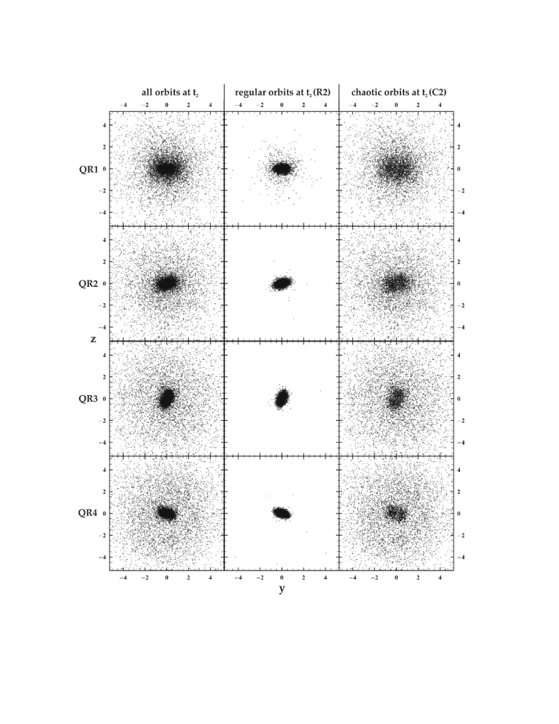
Figure 17: As in Fig. 16, but at $t_{2}=300$. The sets of particles in regular and in chaotic motion found at this snapshot are denoted R2 and C2. About 91%-93% of the identities of the particles in these sets maintain their initial character of motion and belong also to the sets R1 and C1, respectively. Although a spiral pattern cannot be easily seen in these projections, due to the small amplitude of the $m=2$ mode, this mode preserves its spiral pattern even at so late snapshots (see, for example, Fig. 8).

During the evolution of the models from $t_{1}\approx 20$ to $t_{2}=t_{Hub}=300$, most of the particles in R1 or in C1 maintain their character of motion, but some particles change their character of motion from regular to chaotic and some other particles organize their motion from chaotic to regular. Thus, out of the same initial sample, two new sets of particles in regular and in chaotic motion are detected at $t_{2}$. These sets are denoted by R2 and C2 and they are shown in Fig. 17, which is similar to Fig. 16, but for the time $t_{2}$. Spiral arms are not easily discernible in this figures, although we know that even at so late times, as $t_{2}$, the $m=2$ mode has a spiral form at least in the region between the corotation radius and $r\approx 3$ (see Fig. 8). This is because the contrast of the surface density along the spiral arms is so small that cannot be easily recognized simply by projecting a sample of particles on the equatorial plane.

It should be noted that the vast majority (92%-93%) of the identities of particles preserve their initial character of motion (regular or chaotic) up to the end of the Hubble time. They are common in R1 and R2 or in C1 and C2. About $2\%$-$3\%$ of the initially regular orbits become chaotic, and about 5% of the initially chaotic orbits become regular. Also a number of chaotic orbits reduce their Lyapunov numbers during a Hubble time, showing a tendency of self-organization in the system, as discussed above.

The bar in our simulations is formed by the vast majority of regular orbits (about 30%-35%) that remain the same by a factor more that 90% all during the run. This regular part of the bar is surrounded by a layer of chaotic particles (of mass about 10%-15%) that belongs also to the bar (chaotic shell of the bar). There is a continuous exchange of chaotic particles between the bar and the disc. Part of the orbits in the chaotic shell of the bar travel outside the bar (beyond the corotation radius) along the spiral arms or the disc, but a somehow larger number of other chaotic orbits come into the chaotic shell of the bar and they are trapped there, as chaotic (or they organize their motion), so the size of the bar increases in time.

6 Conclusions and discussion

We have presented the results of several N-body simulations of iso-energetic models of galaxies, having different amounts of angular momenta, but the same scalar virial equilibrium. We have examined a number of morphological and dynamical properties of these models and we have found the sets of particles that move in regular or in chaotic orbits in every model. We have compared the spatial distribution of these two sets. Our main conclusions can be summarized as follows:

1) Density waves form a rotating central bar embedded in a rotating thin and a thick disc. The size of the bar decreases and the density in the region of the bar increases with increasing angular momentum of the models.

2) Beyond the ends of the bar an exponential radial profile of the surface density is formed, resembling the observed corresponding profiles of disc galaxies.

3) Spiral arms are spontaneously formed on the disc, due to an $m=2$ spiral wave fluctuation mode on the surface density, excited by the bar. Spiral arms show an intermittent behavior. They are deformed, fade or disappear temporarily, but they grow again, in a time scale less than the rotation period of the bar. The $m=2$ mode preserves its spiral structure outside corotation for a Hubble time, during which the bar describes about 20 to 30 rotations (depending on the angular momentum of the model). The relative amplitude of this mode with respect to higher modes and noise decreases in time. However, in the region of spiral arms the amplitude of $A_{2}(r,t)$ at the end of a Hubble time is on the same level as it is given from observational data.

4) The dynamical rotational velocity curve shows a relatively small variability in a Hubble time indicating a slow redistribution of mass. However, the rotational velocity curve, evaluated from the mean angular momentum of particles inside successive cylindrical rings around the rotation axis, shows a remarkable evolution in time. Namely, this rotation curve decreases in the inner parts, particularly inside one half mass radius, due to the transference of angular momentum outwards.

5) In faster rotating models (as in QR2, QR3, QR4) the central bar loses angular momentum and slows down. The pattern speed $\Omega_{p}$ of the bar decreases in time and the respective corotation radius increases by about $50\%$ at the end of a Hubble time. This result is in good agreement with observational data comparing the linear sizes of young and old bars.

6) Rotation enhances chaos substantially, both by increasing the fraction of mass in chaotic motion and by shifting the Lyapunov numbers to larger values (by about one order of magnitude with respect to the non-rotating model). Two effects collaborate for this enhancement of chaos, both due to rotation. The deformation of the distribution of mass relative to the non-rotating model and the resonant effects, particularly near corotation. The mass that can develop effective chaotic diffusion in a Hubble time increases significantly. In our examples, this mass rises (from the level of 8% of the total mass in the non-rotating Q model) to the level of 45% - 55% in the rotating models.

7) The energies of chaotic orbits are concentrated around the value of the energy near the corotation radius (based on the pattern of the central bar), while the energies of regular orbits are mainly in the deepest part of the potential well.

8) A most remarkable result in this work is that spiral arms are almost completely formed by mass in chaotic motion. This is clearly demonstrated by examining the spatial distribution of the mass in regular and in chaotic motion.

It is significant that in all our models the $m=2$ mode preserves a spiral pattern up to the end of a Hubble time. This mode is gradually obscured by excitation of higher modes and noise. At least part of the power of the higher modes and the noise is expected to be a real effect, but numerical effects are expected to be present as well. We should keep in mind that integrating orbits in a time varying potential is a demanding problem, mainly as regards the accuracy of reproducing the self-consistent potential and its evolution.

In the level of the available accuracy in the dissipationless simulations presented in this paper, our investigation shows only what gravity, combined with rotation, can do. The relative strength of the $m=2$ wave could be better preserved by the end of a Hubble time under the presence of dissipation. Dissipation could absorb noisy components and reinforce the robustness of the $m=2$ mode. Furthermore, gaseous material could be sunk and trapped well inside the corotation radius, as e.g. in Bournaud & Combes (2002); Kormendy & Kennicutt (2004). This process enriches the bar with angular momentum, competing the angular momentum transference outwards.

Other parameters, not involved in this study, could play a role as well. E.g. the presence of a massive central black hole could moderate the strength of the bar (or even destroy the bar, see e.g. Shen & Sellwood 2004). Furthermore, the rate of redistribution of angular momentum can be modified by the presence of a halo with low values of $\lambda$. However, chaos can still play an important role in the dynamics and morphology of these systems.

References

- (1) Allen A.J., Palmer P.L., Papaloizou J., 1990, MNRAS, 242,576.
- (2) Athanassoula E. 2002, ApJ, 569, L83.
- (3) Athanassoula E. 2003, MNRAS, 341, 1179.
- (4) Barnes J., Efstathiou G., 1987, ApJ, 319, 575.
- (5) Binney J., Tremaine S., 1987, Galactic Dynamics. Princeton Series in Astrophysics.
- (6) Block D.L., Buta R., Knapen J.H., Elmegreen D.M., Elmegreen B.G., Puerari I., 2004, AJ, 128, 183
- (7) Buta R., Block D.L., Knapen J.H., 2003, AJ, 126, 1148
- (8) Buta R., Vasylyev S., Salo H., Laurikainen E., 2005, AJ, 130, 506
- (9) Bournaud F., Combes F., 2002, A&A, 392, 83
- (10) Chirikov B.V., 1979, Phys. Rep., 52, 263
- (11) Chirikov B.V., Israilev P.M., Shepelyansky D.L., 1971, Physica D, 33, 77
- (12) Contopoulos G., 1966, ApJ, 144, 1260
- (13) Contopoulos G., 2004, Order and Chaos in Dynamical Systems. Springer.
- (14) Debattista V.P., Sellwood, J.A., 1998, ApJ, 493, L5.
- (15) Debattista V.P., Sellwood, J.A., 2000, ApJ, 543, 704.
- (16) Efstathiou G., Jones B.J.T., 1979, MNRAS, 186, 133.
- (17) Fridman A.M., Khoruzhii O.V., Polyachenko, E.V., 2002, Space Science Reviews, 102, 51
- (18) Gadotti D.A., de Souza R.E., 2005, ApJ, 629, 797
- (19) Gadotti D.A., de Souza R.E., 2006, ApJS, 163, 270
- (20) Gnedin O.Y., Goodman J., Frei Z., 1995, AJ, 110, 1105
- (21) Grosbol P.J., Patsis P., 1998, A&A, 336, 840.
- (22) Innanen K., 1966, ApJ, 143, 150.
- (23) Kalapotharakos C., Voglis N., 2005, Cel. Mech. Dyn. Astr., 92, 157.
- (24) Kalapotharakos C., Voglis N., Contopoulos G., 2004, A&A.,428, 905.
- (25) Kormendy J., Kennicutt R.C. Jr., 2004, ARA&A, 42, 603
- (26) Lin C.C., Shu F.H., 1964, ApJ, 140, 646.
- (27) Lin C.C., Shu F.H., 1966, Proc. Nat. Acad. Sci., 55, 229.
- (28) Linden-Bell D., Kalnajs A.J., 1972, MNRAS, 157, 1.
- (29) Lynden-Bell D., Wood R., 1968, MNRAS, 138, 495
- (30) Muzzio J.C., Carpintero D.D., Wachlin F.C., 2005, Cel. Mech. Dyn. Astr., 91, 173.
- (31) Ohta K., Hamabe M., Wakamatsu K., 1990, ApJ, 357, 710.
- (32) Peebles P.J.E., 1969, ApJ., 155, 393.
- (33) Polyachenko E.V., 2002a, MNRAS, 330, 105
- (34) Polyachenko E.V., 2002b, MNRAS, 331, 394
- (35) Polyachenko V.L., Polyachenko E.V., 2002, Astronomy Reports, 46, 1
- (36) Rosenbluth M.N., Sagdeev R.A., Taylor J.B., Zaslavsky G.M., 1966, Nucl. Fusion, 6, 217
- (37) Shen J., Sellwood J. A., 2004, ApJ, 604, 614
- (38) Skokos Ch., 2001, J. Phys. A: Math. Gen., 34, 10029.
- (39) Tremaine S., Weinberg M., 1984, MNRAS, 209, 729.
- (40) Voglis N., 1994, MNRAS, 267, 379
- (41) Voglis N., 2003, MNRAS, 344, 575
- (42) Voglis N., Hiotelis N., 1989, A&A, 218,1.
- (43) Voglis N., Hiotelis N., Hoflich P. 1991, A&A, 249,5
- (44) Voglis N., Contopoulos G., Efthymiopoulos C., 1998, Phys. Rev. E, 57, 372
- (45) Voglis N., Contopoulos G., Efthymiopoulos C., 1999, Cel. Mech. Dyn. Astr., 73, 211
- (46) Voglis N., Kalapotharakos C., Stavropoulos I., 2002, MNRAS, 337, 619
- (47) Voglis N., Tsoutsis P., Efthymiopoulos C., 2006, MNRAS, submitted, (astro-ph/0607174)
- (48) Walker G.H., Ford, J., 1969, Phys. Rev., 188, 416
- (49) Weinberg M., 1985, MNRAS, 213, 451.
- (50) Zaslavsky G.M., Chirikov B.V., 1972, Sov. Phys. Upsekhi, 14, 549
- (51) Zurek W.H., Quinn P.J., Salmon J.K., 1988, ApJ, 330, 519