HIGH ACCURACY MATCHING OF PLANETARY IMAGES

Abstract

We address the question of to what accuracy remote sensing images of the surface of planets can be matched, so that the possible displacement of features on the surface can be accurately measured. This is relevant in the context of the libration experiment aboard the European Space Agency’s BepiColombo mission to Mercury. We focus here only on the algorithmic aspects of the problem, and disregard all other sources of error (spacecraft position, calibration uncertainties, etc.) that would have to be taken into account. We conclude that for a wide range of illumination conditions, translations between images can be recovered to about one tenth of a pixel r.m.s.

1 Introduction

One of the goals of the European Space Agency’s BepiColombo mission to Mercury is the measurement of the amplitude of the libration of Mercury. In order to do this images of the same surface areas will be taken at different times during the libration cycle and compared. When all other effects—spacecraft position, Mercury’s rotation, spacecraft attitude, etc.—are taken into account, any remaining discrepancy between the positions of features on the surface must be due to the libration of the crust of the planet.

Here we address the question of to what accuracy images can be matched, and we focus only on the algorithmic aspects of the problem, disregarding all other sources of error that would have to be taken into account to solve the scientific problem. We shall show that by using a shape-based matching algorithm images taken under a wide range of illumination conditions can be matched to one tenth of a pixel root-mean-square. Based on this we conclude that the accuracy of the pattern matching algorithm is not the limiting factor in the ultimate accuracy that can be achieved by the libration experiment on BepiColombo.

2 Pattern Matching

The pattern matching algorithms to be used in this study will have to deal with images that may appear to be drastically different from one another, still they refer to the same region. Consider for example the images shown in figure 1. To the human eye it is clear that the images refer to the same region, but any algorithm that relied on the presence of identical features in the images would have great difficulty concluding that the images are related at all.

What is clear by visual inspection is that a number of edges—sharp changes in the level of illumination between contiguous pixels—are common between images. These edges appear where sharp changes in the altimetric profile occur. It is also clear that not all edges appear in all images, owing to the complex interplay between the position of the Sun, and the orientation and slope of the features on the ground.

Compare for instance images b and d in figure 1: the left rim of the crater is bright in one image, and dark in the other. No similar change is observed on the right rim of the crater.

Take now images a and c. Here the left rim of the crater appears almost to be the same, but the extent of the shadow cast by the right rim is dramatically different.

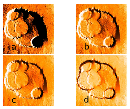
Figure 1: A digital elevation model of Olympus Mons viewed by an imaging camera under different illumination conditions: (a) The Sun is at $\mathit{5}^{\circ}$ elevation; (b) The Sun is at $\mathit{25}^{\circ}$ elevation; (c) The Sun is at $\mathit{50}^{\circ}$ elevation; (d) The Sun is at $\mathit{85}^{\circ}$ elevation. In all cases the Sun’s azimuth is $\mathit{0}^{\circ}$ (to the right).

The ideal algorithm must be able to identify the edges in the two images, must be robust against local, non-linear changes in illumination conditions, and it must be able to operate by identifying a subset of features that are common to the pair of images being compared. Finally, based on the common features identified, the algorithm must be able to recover a possible translation between the two images.

Algorithms that try to minimize the difference between the two, possibly scaled, images are clearly not going to be suited for the task, unless the images to be compared are taken under very similar illumination conditions. While this is possible, it would be a very strong constraint on the operations of a mission.

Based on the considerations above, we have chosen to make use of the image matching algorithms available in the HALCON software library halcon . This is a commercial product used in image vision and image recognition applications.

One particular technique available in the HALCON library is the so-called shape-based matching halcon_manual . This technique is based on an algorithm that identifies the shape of patterns in images, and can be instructed to find in a comparison image the shape identified in a reference image.

2.1 Shape-Based Pattern Matching

The detailed description of the algorithm can be found in the HALCON documentation halcon_manual and has been submitted as part of a European Patent Application espacenet .

The algorithm proceeds through the following steps:

1. A so-called region of interest is identified in the reference image. This is a region of the image where edges will be looked for. The region of interest must be selected to be fully contained in both images. This step is done by hand, based on some a priori knowledge, or visual inspection of the images. In our case, where the simulated translations amount to a few pixels along either or both the X and Y axes (see § 5), the region of interest is the whole reference image, minus a few pixels around the edges. In the case of two partially overlapping images of the same region one would choose the intersection of the two images.

2. Features are identified in the comparison image with an edge detection algorithm. Pixels identified by the edge detection algorithm are part of the reference pattern.

3. The edge detection algorithm is run on the comparison image. This results in a second collection of pixels, the search pattern.

4. The algorithm now overlays the reference pattern on the search pattern. The reference pattern is stepped over the search pattern in an attempt to maximize the number of overlapping pixels. In doing so the algorithm is allowed to reduce the number of pixels in the reference pattern. The maximum fraction of the search pattern that can be discarded in the process can be set by the user. In our application the reference and search patterns can differ vastly. Therefore we have allowed the algorithm to throw away up to $70\,\%$ of the pixels. In trying to maximize the overlap between the two patterns, the algorithm can be instructed to allow for a rotation and a scaling factor.

5. The algorithm reports the recovered translations and the fraction of the pixels in the reference pattern that was used to find a match. The latter is called the score. Within the parameters given by the user, the algorithm always chooses the match with the highest score.

2.1.1 The Meaning of the Score

The HALCON score is the normalized sum of the cross product between the vectors describing the position of the pixels in the reference pattern and those describing the pixels in the search pattern. If the two patterns are identical, it is clear that the score will be equal to one. When pixels have to be dropped from the reference pattern, the score will decrease.

In the actual algorithm, the sum of the cross products of the pixels used in the match is slightly modified to take into account the possibility of non-linear changes in the illumination conditions, either locally, around certain features, or globally, across the entire image espacenet .

It is tempting to interpret the HALCON score as a quality factor for the goodness of the translation parameters found. However this would be wrong on two counts.

First of all, it is clear that often only a subset of the pattern to be looked for is to be found in the search pattern. (Refer back to the examples shown in figure 1.) In this case the search algorithm must discard some of the pixels in the reference pattern in order to find a good matching sub-pattern. How many pixels are left in the sub-pattern has nothing to do with whether the match is good or not.

Second, the notion of goodness of match implies that the matched pattern can be compared to an expected result, or true pattern, or that the algorithm proceeds through the optimization of an objective function. But the only measure of how well the algorithm has performed, is how close the recovered translation is to the values injected in the simulation. This means that the accuracy of the algorithm can only be judged through an extensive set of Monte Carlo simulations. Only by repeatedly comparing two images in multiple realizations of the same detection and matching process, is it possible to gauge the statistical errors in the results, and therefore establish to what accuracy and under what conditions the algorithm can be effectively employed.

3 Approach

The following steps were identified.

1. Render a digital elevation model of the surface of a planet, by choosing the position of the Sun and of the spacecraft. We have used povray povray for this task.

2. Create two images, the reference image and the comparison image. The latter is possibly translated along one or both of the image axes.

3. Convert the rendered images to instrument count images of a given signal-to-noise ratio.

4. Recover translation parameters between the two images using a shape-based pattern matching algorithm.

5. Study the accuracy with which the parameters are recovered, and derive information on the range of illumination conditions for which the parameters can be successfully recovered.

4 Digital Elevation Models

Four digital elevation models have been used in this study. These are shown in figure 2.

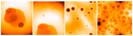
Figure 2: The four digital elevation models used in this study. From left: The Olympus Mons caldera; a bowl-shaped crater close to the Olympus Mons caldera; a synthetic landscape with several bowl-shaped craters; another synthetic landscape containing approximately 5000 craters. (An image of Mercury taken from an height of 400 km might contain a few thousands of craters with a diameter larger than a few tens of meters.) Darker colors represent lower elevations.

5 Simulation Runs

After some preliminary simulations used to determine a useful sampling scheme of the parameter space, the bulk of the simulations were carried out with the following parameters values:

• Translations: 100 meter in X, in Y, and in X and Y.

• Sun elevation angles: 10^∘, 30^∘, 60^∘, 90^∘.

• Nominal spacecraft height 1500 km .

• Sun azimuth angle: several (the same azimuth angle for reference and comparison images). For one model a difference in azimuth of $30^{\circ}$ between the two images was introduced.

• Four digital elevation models rendered with a signal-to-noise ratio of 50. The signal-to-noise ratio is determined when the Sun is at the zenith.

6 Results

For each digital elevation model used, several thousand data points have been calculated. Each data point refers to a particular combination of Sun elevation and azimuth for the reference and comparison images, and a translation along one or both of the image axes. For each combination of parameters, the same number of simulation runs (ten) was carried out.

In the following we use $\Delta_{x}$ and $\Delta_{y}$ to indicate the difference between the amplitude of the translation recovered by the algorithm and the amplitude of the translation used in the simulation. Therefore the expectation value of $\Delta_{x}$ and $\Delta_{y}$ is always 0, and the width of their distributions is a measure of the statistical error in the reconstruction.

In table 1 we give a summary of how successful the algorithm has been. For each digital elevation model we give the number of realizations (all Sun angles and all translations), how many times the algorithm failed to return a match, and how many times the returned result was more than 2 pixels away from the expected result. The latter figure has no special meaning, but is meant to give an idea of the global behavior of the algorithm.

DEM	Total	No match	$\Delta_{x}>2$ or $\Delta_{y}>2$
A	9878	$2.8\%$	$2.3\%$
B	7300	$3.2\%$	$4.2\%$
C	6254	$0\%$	$12.6\%$

Table 1: Global success statistics for the simulation runs. For each digital elevation model (DEM) the following data are reported: the total number of independent realizations; the fraction of realizations for which the algorithm was not able to find any match; the fraction of realizations for which either $|\Delta_{x}|$ or $|\Delta_{y}|$ were larger than two pixels. DEM keys: A = Olympus Mons, B = bowl crater, C = synthetic.

One thing is immediately apparent: for the synthetic digital elevation model the algorithm always returned a match, but a larger fraction of the returned answers was significantly wrong. Because the synthetic model is significantly more regular than the other two — in particular the craters are identical but for a scale factor, the algorithm has an easier job at finding some matching pattern, although relatively more often the pattern found is not the good one.

Based on these observations, we present the results for the synthetic model separately. However, we will be able to show that the same conclusions on the accuracy of the algorithm can be reached for all digital elevation models by applying the same selection criteria on the illumination conditions.

In the following sections we use the following notation:

• $\theta_{cut}$ refers to the following selection: $\theta_{sun}>10^{\circ}$ and $\theta_{sun}\neq 90^{\circ}$ , where $\theta_{sun}$ is the Sun elevation angle in the reference or the comparison image.

• $\phi_{cut}$ refers to the following selection: $|\phi_{sun}-n\times 90^{\circ}|>20$ for $n\in{0,1,2,3,4}$ , where $\phi_{sun}$ is the Sun azimuth — this is the same in both the reference and the comparison images.

6.1 The Olympus Mons Models

Most of the high-deviation points come from images where the Sun elevation is equal to $90^{\circ}$, or images where the Sun elevation is lower than $10^{\circ}$ ($\theta_{cut}$). This is shown in figure 3.

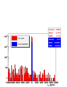
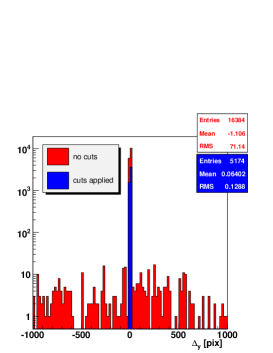
Figure 3: The effect of the Sun elevation cut on the distribution of $\Delta_{x}$ (top) and $\Delta_{y}$ (bottom) for the Olympus Mons data.

In figure 4 we plot the data with $\theta_{cut}$ applied versus the Sun azimuth. We observe that the mean of $\Delta_{x}$ and $\Delta_{y}$ vary with $\phi_{sun}$ in a quasi-periodic fashion. What we observe is that the deviation is larger when the Sun azimuth is orthogonal to one of the image axes. Namely, the largest deviations for $\Delta_{x}$ are observed when $\phi_{sun}\approx 90^{\circ}$ or $270^{\circ}$, whereas the largest deviations for $\Delta_{y}$ are observed when $\phi_{sun}\approx 0^{\circ}$ and $180^{\circ}$ . The direction defined by the Sun azimuth appears to be a preferential direction: translations along this direction can be more accurately recovered, because the features on the terrain create sharper shadows along the direction to the Sun.

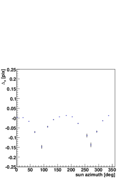
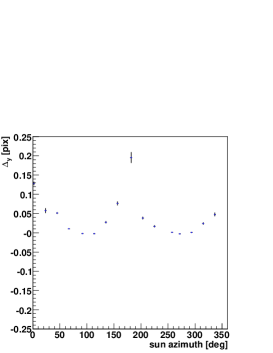
Figure 4: The average $\Delta_{x}$ and $\Delta_{y}$ versus the Sun azimuth for the Olympus Mons data. The error bar on each point represents the root-mean-square.

Based on the data in figure 4 we can devise a selection criterion for the Sun azimuth, so that translations along both axes can be recovered with comparable accuracy. The selection criterion is that the Sun azimuth must be more than $20^{\circ}$ away from both image axes. The distributions of $\Delta_{x}$ and $\Delta_{y}$ when both $\theta_{cut}$ and $\phi_{cut}$ are applied are shown in figure 5.

Figure 5 represents the end point of our analysis. We observe that the two distributions are centered on 0, and have a width of $\approx$ 0.1 pixel root-mean-square. The two distributions have a tail in the direction of the translation applied in the simulations (-100 m along the X axis, and +100 m along the Y axis). The nature of this slight asymmetry in not understood at present.

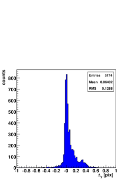
Figure 5: The distribution of $\Delta_{x}$ and $\Delta_{y}$ for the Olympus Mons data, once both the Sun cuts are applied.

6.1.1 Changing the Sun Azimuth

The bulk of the simulation runs was carried out with the same Sun azimuth for both the reference and comparison images. We however also made a set of simulation runs where the azimuth of the Sun in the comparison image was $30^{\circ}$ away from the azimuth used in the reference image; only a translation of 100 meters along the X axis was applied. The results are shown in figure 6. Even in this case the algorithm is able to recover the injected translation with an accuracy of $\approx$ 0.1 pixel root-mean-square.

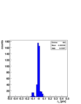
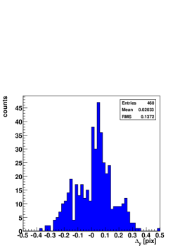
Figure 6: The distribution of $\Delta_{x}$ (top) and $\Delta_{y}$ (bottom) for the Olympus Mons data for date where the Sun azimuth of the comparison and reference images differ by $30^{\circ}$.

6.2 The Synthetic Model

As already hinted to, the results based on the synthetic digital elevation model give a slightly different picture, although the main conclusions do not change.

The $\theta_{cut}$ criterion is still effective in rejecting data points that return a large deviation from the expectation.

A point of discrepancy with respect to the Olympus Mons data is the behavior of the recovered translations as a function of Sun azimuth. Figure 7 shows that the effect observed for the Olympus Mons models is almost not observed here. After the $\theta_{cut}$ criterion is applied, any remaining offset is smaller than 0.05 pixel.

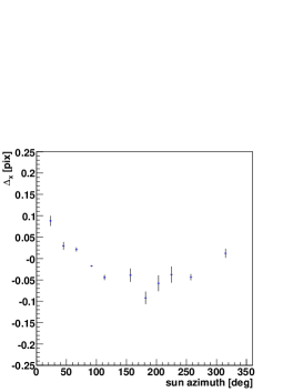
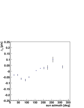
Figure 7: The average $\Delta_{x}$ (top) and $\Delta_{y}$ (bottom) versus the Sun azimuth for the Synthetic Model data. The error bar on each point represents the root-mean-square.

Finally, figure 8 shows the distribution for $\Delta_{x}$ and $\Delta_{y}$. Again, the translation is recovered with an accuracy of $\approx$ 0.1 pixel root-mean-square, but the details of the distributions differ from what was observed before.

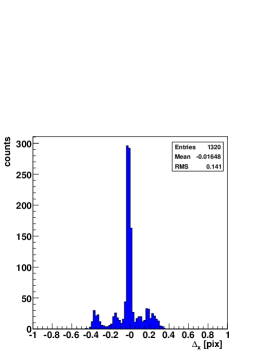
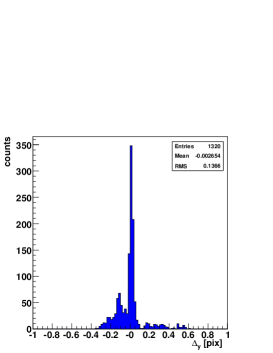
Figure 8: The distribution of $\Delta_{x}$ (top) and $\Delta_{y}$ (bottom) for the Synthetic Model data, once both the Sun cuts are applied.

7 Conclusions

We have performed a study of the accuracy with which a shape-based pattern matching algorithm can identify translations between remote sensing images of the same planetary features. We have applied the algorithms in a Monte Carlo fashion to digital elevation models (both real and synthetic) in order to investigate the statistical performance of the procedure.

We find that for a broad range of illumination conditions translations between images can be recovered with an accuracy of 0.1 pixel r.m.s.

The algorithm performs best for translations along the projected direction to the Sun on the image plane. This study shows that translations along both image axes at the same time can be recovered with the same accuracy of 0.1 pixel as long as the projected direction to the Sun lies more than $\approx 20^{\circ}$ away from the same image axes.

Finally, this study demonstrates that the images to be compared need not be taken under the very same illumination conditions in order to be effectively matched. For a given Sun azimuth, any pair of images taken with Sun elevation angles larger than $10^{\circ}$ can be used; images taken when the Sun is at the zenith must also be avoided. The range of useful illumination conditions is further broadened because this study concludes that differences in Sun azimuth of at least $30^{\circ}$ do not affect the accuracy of the matching algorithm.

The error contributed by the matching algorithm is but one of the several error contributions to be taken into account during the analysis of the data pertaining to the measurement of the possible libration of the surface of Mercury. This study shows that the accuracy of the pattern matching algorithm is not a limiting factor in the ultimate accuracy of the libration experiment aboard the BepiColombo mission to Mercury.

References

- (1) HALCON Documentation. http://www.mvtec.com/halcon/.
- (2) HALCON Manual. http://www.mvtec.com/download/documentation/.
- (3) EP1193642, April 2002. http://www.espacenet.com/.
- (4) Persistence Of Vision Raytracer. http://www.povray.org/.