Measuring the Average Evolution of Luminous Galaxies at $z<3$: The Rest-frame Optical Luminosity Density, Spectral Energy Distribution, and Stellar Mass Density

Abstract

We present the evolution of the volume averaged properties of the rest-frame optically luminous galaxy population to $z\sim 3$, determined from four disjoint deep fields with optical to near-infrared wavelength coverage. Our use of independent lines of sight substantially mitigates field-to-field variations. We select galaxies above a fixed rest-frame $V$-band luminosity of $3\times 10^{10}$${\rm~{}h_{70}^{-2}~{}L_{\odot}}$ and characterize their rest-frame ultraviolet through optical properties via the mean spectral energy distribution (SED). To measure evolution we apply the selection criteria to a sample of galaxies from the Sloan Digital Sky Survey (SDSS) and COMBO-17 survey. The mean rest-frame 2200${\rm\AA}$ through $V$-band SED becomes steadily bluer with increasing redshift but at all redshifts $z<3$ the mean SED falls within the range defined by “normal” galaxies in the nearby Universe. Rest-frame 4000Å/Balmer breaks are present in the volume averaged SED at all redshifts, indicating significant light and mass contributions from evolved populations, even at $z\sim 2.8$. We measure stellar mass-to-light ratios (${\cal M_{\star}}/{\rm L}$) by fitting models to the rest-frame UV-optical SEDs. Multiplying our volume averaged ${\cal M_{\star}}/{\rm L}_{V}$ estimates at each redshift by the measured mean $V$-band luminosity density, we derive the stellar mass densities $\rho_{\star}$. The stellar mass density in galaxies selected at a fixed luminosity has increased by a factor $3.5-7.9$ from $z=3$ to $z=0.1$, where the range includes the uncertainty due to field-to-field variance within our own data. If we use our observed ${\cal M_{\star}}/{\rm L}_{V}$ evolution to select galaxies at a fixed mass, the stellar mass density evolves by a factor of $5.3-16.7$. After correcting to total, the measured mass densities at $z<2$ lie below the integral of the star formation rate (SFR) density as a function of redshift as derived from UV selected samples after a standard correction for extinction. This may indicate a systematic error in the total $\rho_{\star}$ or SFR($z$) estimates. We find large discrepancies between recent model predictions for the evolution of $\rho_{\star}$ and our results, even when our observational selection is applied to the models. Finally we determine that Distant Red Galaxies (selected to have $J_{s}-K_{s}>2.3$) in our ${\rm L}_{V}^{rest}$ selected samples contribute $30\%$ and 64% of the stellar mass budget at $z\sim 2$ and $z\sim 2.8$ respectively. These galaxies are largely absent from UV surveys and this result highlights the need for mass selection of high redshift galaxies.

1. Introduction

Our knowledge of the high redshift Universe has increased rapidly over the past decade and is becoming ever more comprehensive. The initial large advances in this field were enabled by the efficient selection of $z\sim 3$ starforming galaxies based on their optical light, e.g. Steidel et al. (1996) and Steidel et al. (1999), and by the development of efficient multi-object spectrographs on large 8-10m class telescopes. Objects selected by these techniques allowed us for the first time to study statistically significant samples of galaxies at $z>1.5$. Resultant follow-up work on these optically (rest-frame ultraviolet; UV) selected objects at $z\sim 3$ (Lyman Break Galaxies; LBGs) and subsequent samples at $z\sim 2$ (BM/BX objects; Steidel et al. 2004; Adelberger et al. 2004) have demonstrated that these galaxies have generally low extinctions $E(B-V)\sim 0.15$ and modest ages ($<1$ Gyr) and stellar masses ($\cal{M_{\star}}$$\sim 10^{10}$${\cal M_{\odot}}$) with a tail to high end values existing at bright $K$ magnitudes, e.g. Sawicki, Lin, & Yee (1997), Papovich, Dickinson, & Ferguson (2001; hereafter P01), Shapley et al. (2001), Shapley et al. (2005), Reddy et al. (2005).

Although efficient in telescope time for observing objects with $R\lesssim 25$, optical surveys will miss objects that have high extinctions or those with a lack of current vigorous star formation. In fact, most galaxies with $\cal{M_{\star}}$$\gtrsim 10^{11}$${\cal M_{\odot}}$ have optical magnitudes too faint for optical spectroscopic followup (van Dokkum et al., 2006). A comprehensive view of the high redshift Universe requires that UV selection be complemented with selection from light at least as red as the NIR, which corresponds to the rest-frame optical out to $z\sim 3$. Deep NIR observations allow us to detect highly extincted (e.g. SCUBA galaxies; Smail et al. 1997) or passive galaxies at $z>1.5$ (e.g. Daddi et al. 2005), which have very little rest-frame UV emission.

However, getting deep NIR data is observationally expensive and even over small fields requires substantial investments of 8-10m telescope time to reach depths fainter than $K_{s}$$=20-21$. Until the recent development of megapixel NIR arrays progress was measurable but slow, e.g. Hogg et al. (1997) and Bershady et al. (1998). A large step forward was taken with the Faint Infrared Extragalactic Survey (FIRES; Franx et al. 2000; Rudnick et al. 2001; Labbé et al. 2003; Förster Schreiber et al. 2005) and with the NICMOS observations of the Hubble Deep Field North (HDF-N; P01; Dickinson et al. 2003). FIRES is an ESO large program which imaged in $J_{s}$, $H$, and $K_{s}$ the HDF-S and a field centered around the x-ray luminous cluster MS1054-03 at $z=0.83$. At the time these fields had a unique combination of area and deep HST optical imaging and the ESO data extended this coverage to the $K_{s}$-band. The FIRES data were particularly valuable because the associated deep $K_{s}$-band data provide access to the rest-frame $V$-band all the way out to $z\sim 3$. The very deep FIRES data allowed us to probe rest-frame $V$-band luminosities ${\rm L}_{V}^{rest}$ down to $\sim 50\%$ of the local ${\rm L}^{\star}_{V}$ value.

The powerful combination of very deep NIR and optical data now make it possible to assemble representative samples of the Universe at $z>1.5$. For example, Franx et al. (2003) and van Dokkum et al. (2003) have shown that galaxies selected to have $(J_{s}-K_{s})$$>2.3$ are luminous in the rest-frame optical, likely have high $\cal{M_{\star}}$, but would be almost completely missed by rest-frame UV selected surveys. Subsequent studies of these Distant Red Galaxies (DRGs) have shown that they have systematically older ages, higher extinctions, higher $\cal{M_{\star}}$, and comparable or even higher star formation rates than the optically selected LBGs at comparable redshifts and $K$ magnitudes (van Dokkum et al., 2004; Förster Schreiber et al., 2004; Labbé et al., 2005; Papovich et al., 2005; van Dokkum et al., 2006) and may contribute significantly to the stellar mass density at $z>1.5$ (Rudnick et al. 2003 – hereafter R03). Other author have also found galaxy populations that would be missed by rest-frame UV selection, highlighting the need for a comprehensive selection of galaxies (e.g. Daddi et al. 2004).

While individual properties of galaxies are indeed important, for some quantities the modeling of the volume averaged population may yield more robust results. For example R03 demonstrated that bursty SFHs cause a smaller systematic error in the mean stellar mass-to-light ratio ${\cal M_{\star}}/{\rm L}$ of the galaxy population - and hence estimates of $\rho_{\star}$ - than when it is determined from averages of ${\cal M_{\star}}/{\rm L}$ estimates of individual galaxies. The utility of using cosmically averaged quantities has also been demonstrated by other authors across a range of topics. Using the luminosity density determinations at many wavelengths Madau, Pozzetti, & Dickinson (1998) tried to constrain the shape of the cosmic SFH by fitting the different bands simultaneously. Pei, Fall, & Hauser (1999) derived independent constraints on the cosmic SFH by modeling the cosmic gas content, metallicity, and extragalactic background light. Using the FIRES data on the HDF-S R03 modeled the rest-frame optical mean colors and luminosity densities to derive the evolution in the stellar mass density at $z<3$. At low redshifts Baldry et al. (2002) and Glazebrook et al. (2003) modeled the mean galaxy spectrum from 2dF and the Sloan Digital Sky Survey (SDSS; York et al. 2000) to constrain the cosmic SFH.

Using the deepest existing $K_{s}$-band data R03 showed for the HDF-S that the evolution in the volume averaged rest-frame optical colors, e.g. $(U-B)_{rest}$, $(B-V)_{rest}$, and $(U-V)_{rest}$, at $z<3$ was monotonic, with bluer colors at higher redshifts. The colors also lay close to the locus of colors occupied by individual normal galaxies in the local Universe (Larson & Tinsley, 1978; Jansen et al., 2000a). They also found that the evolution in the rest-frame colors could be approximated by smooth SFHs with a constant metallicity and dust. Models with these SFHs were then used to convert the $(U-V)_{rest}$ to ${\cal M_{\star}}/{\rm L}_{V}$ and hence to a mass density.

A primary goal of this paper is to extend the analysis of R03. One major area of improvement is that this paper will model the full rest-frame UV through optical volume averaged SED of luminous galaxies in the Universe, allowing more freedom in the choice of dust attenuation, SFH, and age. The full rest-frame UV through optical information also gives us more insight as to the nature of the mean stellar population of luminous galaxies at high redshift. Perhaps the most important improvement with respect to R03 is that we include data from four disjoint fields, covering a total area of $\approx 98.8$ arcminutes. This is crucial since the field-to-field variations in the number densities of galaxies are expected to be large in small fields. In addition, multiple fields are important to characterize the mean contribution of different galaxy populations, e.g. DRGs, to the volume averaged SED and $\rho_{\star}$. For example the field-to-field variations in the number densities of DRGs is known to be high with large differences between the HDF-N and HDF-S (Labbé et al. 2003; hereafter L03).

In this paper we combine FIRES data from the HDF-S and MS1054-03 fields with those from the HDF-N catalog of P01 and D03 and a catalog from the Great Observatories Origins Deep Survey (GOODS) images of the Chandra Deep Field South (CDF-S; Wuyts et al. in preparation). Using photometric redshifts from these four catalogs we derive the rest-frame luminosities, luminosity densities and colors. We examine the trends in color and redshift and compute the full rest-frame 2200${\rm\AA}$ through $V$-band volume averaged SED. We then apply the same analysis to a galaxy sample from SDSS and from the COMBO-17 survey and use it to derive the evolution of mean SED properties in a consistent manner from $z\sim 3$ down to $z=0$. Finally, we fit the full rest-frame mean SED with a set of simple models and use these to derive the mean ${\cal M_{\star}}/{\rm L}_{V}$ and $\rho_{\star}$ in each redshift bin.

In § 2 we describe the data. In § 3 we review the methods that we use to calculate photometric redshifts, rest-frame luminosities, luminosity densities, and global colors. In § 4 we present the results including the evolution of the rest-frame luminosity density, color, and volume averaged SED. In this section we also present the model fits to the mean SED and the derived ${\cal M_{\star}}/{\rm L}$ and $\rho_{\star}$ evolution. We discuss these results in § 5 and present our conclusions and summary in § 6. Throughout this paper we assume $\Omega_{\mathrm{M}}=0.3,~{}\Omega_{\Lambda}=0.7,~{}\mathrm{and~{}H_{o}}=70~{}{\rm h_{70}~{}km~{}s^{-1}Mpc^{-1}}$ unless explicitly stated otherwise.

2. The Data

We combine results from four different fields: the HDF-S, MS1054-03, HDF-N, and CDF-S. Below we briefly describe the data reduction and the construction of catalogs. All magnitudes are quoted in the Vega system unless specifically noted otherwise. Our adopted conversions from Vega system to the AB system are $J_{s,vega}$ = $J_{s,{\rm AB}}$ - 0.90, $H_{vega}$ = $H_{{\rm AB}}$ - 1.38, and $K_{s,vega}$ = $K_{s,{\rm AB}}$ - 1.86 (Bessell & Brett, 1988).

2.1. FIRES Data

The reduced images and photometric catalogs for the two FIRES fields are available online through the FIRES homepage at
http://www.strw.leidenuniv.nl/$\sim$fires.

2.1.1 The HDF-S

A complete description of the FIRES HDF-S observations, reduction procedures, and the construction of photometric catalogs is presented in detail in L03; we outline the important steps below.

The FIRES data on the WFPC2 field of the HDF-S is comprised of 101.5 hours of exposure with ISAAC (Moorwood, 1997) on the VLT. These exposures were split into 33.6, 32.3, and 35.6 hours in $J_{s}$, $H$, and $K_{s}$ respectively. The data were taken in service mode at the VLT and have a mean image quality better $0\farcs 48$ in all bands. These NIR data were combined with the very deep optical data from WFPC2 taken by Casertano et al. (2000).

Objects were detected in the $K_{s}$-band image with version 2.2.2 of the SExtractor software (Bertin & Arnouts, 1996). For consistent photometry between the space and ground-based data, all images were then convolved to $0\farcs 48$, corresponding to the effective resolution of the NIR band with the worst average seeing. Photometry was then performed in the $U_{300}$, $B_{450}$, $V_{606}$, $I_{814}$, $J_{s}$, $H$, and $K_{s}$-band images using specially tailored isophotal apertures defined from the detection image. In addition, a measurement of the total flux in the $K_{s}$-band, $K_{s}^{\rm tot}$, was obtained using an aperture based on the SExtractor AUTO aperture, which includes a conservative aperture correction. The effective area of the HDF-S is 4.74 square arcminutes, including only areas of the chip with exposure time $\geq 20\%$ of the total integration time in all bands. The accuracy of photometric redshifts (to be discussed in §3.1) and rest-frame optical luminosities in our $K_{s}$-selected sample is very dependent on the quality of the NIR data (e.g. Rudnick et al. 2001) and once the S/N in the NIR bands becomes too low the quality of the photometric redshifts becomes too poor for a useful analysis. Since the $K_{s}$-band is our shallowest NIR band a cut there is a conservative proxy for a cut in the S/N of the other NIR bands, keeping in mind the range of galaxy NIR colors. The final catalog has 358 objects with $K_{s}^{\rm tot}$$<23.14$, which for point sources corresponds to a 10$\sigma$ S/N in the custom isophotal aperture.

2.1.2 The MS1054-03 Field

The MS1054-03 observations, data reduction, and catalog construction are described in detail in Förster Schreiber et al. (2006). This field has an x-ray detected cluster at $z=0.83$ and at the time of the FIRES proposal was the field with the best combination of depth and area observed with WFPC2. The WFPC2 data in $V_{606}$ and $I_{814}$ are presented in van Dokkum et al. (2000). The FIRES observations of this field consisted of 78 hours of $J_{s}$, $H$, and $K_{s}$ imaging with ISAAC, supplemented with $UBV$ imaging with FORS1 on the VLT. The observations were split over four pointings. The total effective area is 23.5 square arcminutes, including only those pixels with exposure time $\geq 20\%$ of the total integration time in all bands. Observing conditions in the MS1054-03 field were generally similar to the HDF-S and since the exposures were split over 4 pointings the depth is 0.7 magnitudes shallower than in the HDF-S.

Object detection and catalog construction were performed in an identical way as in the HDF-S. The final catalog has 1380 sources with $K_{s}^{\rm tot}$$<22.34$, which also corresponds roughly to a 10$\sigma$ detection for point sources.

2.2. HDF-N

The WFPC2 data on the HDF-N are presented in Williams et al. (1996). The data reduction of the NICMOS $J_{110}$ and $H_{160}$ data and the Kitt Peak $K_{s}$ data is described by Dickinson (1999) and Dickinson et al. (2000) as is the catalog construction. Objects were detected in a weighted sum of the $J_{110}$ and $H_{160}$ images, which are individually much deeper than the $K_{s}$-band image. The HST $U_{300}$, $B_{450}$, $V_{606}$, $I_{814}$, $J_{110}$, and $H_{160}$ data were then convolved to the same PSF and the fluxes were measured in matched apertures. The ground-based $K_{s}$ data, which has much worse image quality, was extracted using the “TFIT” method described in P01 to achieve consistent colors between the space-based and ground-based images. A total magnitude in the $H_{160}$-band was estimated using the SExtractor AUTO aperture. The area of the HDF-N is 5 square arcminutes. The final catalog has 854 sources with $H_{160}^{\rm tot}$(AB)$<26.5$.

The HDF-N is unique among our fields in that the the detection is not done in the $K$-band. Nonetheless, the $H_{160}$-band data are sufficiently deep so that we are complete to the rest-frame $V$-band luminosity limit above which we select galaxies for this study (see § 3.2).

2.3. CDF-S

From GOODS/EIS observations of the CDF-S (data release version 1.0) a $K_{s}$-band selected photometric catalog is constructed, described by Wuyts et al. (in preparation). ISAAC imaging on the VLT provides 72 hours of exposure in $J$, 55 in $H$ and 122 in $K_{s}$, split over 21, 12 and 23 pointings respectively. GOODS zeropoints were adopted for $J$ and $K_{s}$. The $H$-band zeropoint was obtained by matching the stellar locus on a $J-K$ vs $J-H$ color-color diagram to the stellar locus in HDF-S and MS1054. The difference with the official GOODS $H$-band zeropoint varies across the CDF-S but on average our $H$-band zeropoints is $\approx 0.1$ magnitudes brighter. ACS imaging provides photometry in $B_{450}$, $V_{606}$, $I_{814}$, and $z_{850}$ bands. All images were smoothed to match the NIR pointing with the worst seeing, $0\farcs 64$. Identical procedures as in the HDF-S and MS1054 fields were applied to detect objects and construct the catalog. A total effective area of 65.6 square arcminutes is well exposed in all bands. The final catalog contains 1588 objects with $K_{s}^{\rm tot}$$<21.34$ in this area. At $K_{s}^{\rm tot}$$=21.34$ the median S/N in the $K_{s}$ isophotal aperture is $\sim 12$.

2.4. DRG selection

Because the depth across our four fields is non-uniform we do not consistently apply a magnitude selection for DRGs. This may produce a slight error when comparing the DRGs to non-DRGs in each field. In addition, DRGs have different magnitude distributions in the different fields (Förster Schreiber et al., 2004) and this may slightly bias the mass budgets determined in §4.4.1. In all fields our limiting $K_{s}$ magnitude for DRG selection was dictated by the depth of our $J_{s}$ data, which must be deep enough so that non-detections in $J_{s}$ can still be selected as DRGs.

In all fields DRGs were selected to have $z_{phot}>1.5$. In the HDF-S 12 DRGs were selected to have $J_{s}-K_{s}>2.3$, $K_{s}^{\rm tot}$$<22.5$ and $z_{phot}>1.5$. In the MS1054-03 field 31 DRGS were selected at $K_{s}^{\rm tot}$$<21.7$. The brighter $K_{s}$ limit in comparison to the HDF-S is a direct result of the shallower data. In the CDF-S 65 DRGs were selected with $K_{s}^{\rm tot}$$<21.14$. This is 0.2 magnitudes shallower than the CDF-S catalog depth to insure reliable colors for objects that are red in $(J_{s}-K_{s})$.

We select DRGs in the HDF-N to have $K_{s}^{\rm tot}$$<21.05$, which corresponds to a 5-$\sigma$ detection in $K_{s}$. The very deep NICMOS $J_{110}$ observations allow robust color measurements of red objects at this $K_{s}$ limit. The selection of DRGs in the HDF-N is complicated, however, by the use of the $J_{110}$ filter, which is significantly bluer (effective wavelength of $1.13\mu m$ for $J_{110}$ and $1.25\mu m$ for $J_{s}$) and about twice as broad (c.f. the NICMOS Instrument Handbook). It is therefore not appropriate to select DRGs using a $J_{110}-K_{s}>2.3$ color cut. Instead we compute a synthetic $J_{s}-K_{s}$ color using our best fit photometric redshift template (see §3.1) to derive the $J_{s}$ magnitude. To assess the reliability of this method we first synthesize the $J_{110}-K_{s}$ color and compare it the observed color. At $K_{s}^{\rm tot}$$<21.05$ the outlier resistant normalized absolute median deviation ($\sigma_{NMAD}$; equal to the rms for a Gaussian distribution) in the colors is 0.05 for all sources and 0.14 for those sources at $1.6<z<3.5$. Computing the synthetic $J_{s}-K_{s}$ color for every galaxy we find two DRGs in the HDF-N with $1.6<z<3.5$.

3. Methods

3.1. Photometric Redshifts and Rest-Frame Luminosities

Photometric redshifts $z_{phot}$ for all galaxies are derived using an identical code to that presented in Rudnick et al. (2001) and R03 but with a slightly modified template set. This code models the observed SED using non-negative linear combinations of a set of 8 galaxy templates. As in R03 we use the E, Sbc, Scd, and Im SEDs from Coleman, Wu, & Weedman (1980), the two least reddened starburst templates from Kinney et al. (1996) and a synthetic template corresponding to a 10 Myr year old simple stellar population (SSP) with a Salpeter (1955) stellar initial mass function (IMF). In this paper we have added a 1 Gyr old SSP with a Salpeter IMF.

Using spectroscopic redshifts $z_{spec}$ we have determined that $\sigma_{NMAD}(z_{spec}-z_{phot}~{}/~{}(1+z_{spec})=0.06$, 0.06, and 0.08 at $z<4$, $0<z<1.5$, and $1.5\leq z<4$ respectively.

It is important to remember, however, that the spectroscopic samples in the HDF-S and HDF-N are highly biased toward UV bright objects at high redshift, e.g. LBGs. In the MS1054-03 and CDF-S field spectroscopy has been performed on $K_{s}$ selected sources and those selected to be red in $J_{s}-K_{s}$ and in $I-H$. The photometric redshift accuracy for DRGs is $\sigma_{NMAD}=0.11$ and 0.09 in in MS1054 and the CDF-S respectively. There are, however, very few DRGs with secure $z_{spec}$ measurements (4 in MS1054-03 and 3 in the CDF-S) causing the determination of the $z_{phot}$ accuracy itself to be uncertain at this point. From these first determinations, the accuracy of the $z_{phot}$ measurements is still adequate for the construction of the luminosity densities and colors that we use here.

The two sided 68% confidence intervals on $z_{phot}$, i.e. $\delta z_{phot}$, are computed using the monte carlo simulation described in R03. In general the differences between $z_{phot}$ and $z_{spec}$ are well reflected by $\delta z_{phot}$. $\delta z_{phot}$ can therefore be used to judge the reliability of the $z_{phot}$ estimates.

Rest-frame luminosities are computed using the method described in the appendix of R03. We compute rest-frame luminosities ${\rm L^{rest}_{\lambda}}$ in two UV bands centered approximately at 2200 and 2700${\rm\AA}$. These filters correspond to the $ST-UV22$ and $ST-UV27$ filters from (Bruzual & Charlot 2003; hereafter BC03). In addition we compute rest-frame luminosities in the $UX$, $B$, $V$, $R$, and $I$ filters of Bessell (1990). For these filters we use $M_{\odot,U}=+5.66$, $M_{\odot,B}=+5.47$, $M_{\odot,V}=+4.82$, $M_{\odot,U}=+4.28$, and $M_{\odot,U}=+3.94$. For each galaxy we only compute ${\rm L^{rest}_{\lambda}}$ in rest-frame filters that are at shorter observed wavelengths than the $K_{s}$ filter. In all cases where a spectroscopic redshift is available we compute the rest-frame luminosities fixed at $z_{spec}$.

3.1.1 Star Identification

Stars in all four fields were identified by spectroscopy, by fitting the object SEDs with stellar templates from Hauschildt, Allard, & Baron (1999), and by inspecting their morphologies, as in R03. In well exposed regions of the HDF-S, MS1054-03, HDF-N, and CDF-S data we identified 29, 68, 16, 236 stars respectively down to $K_{s}^{\rm tot}$$<23.14$, $K_{s}^{\rm tot}$$<22.34$, $H_{160}^{\rm tot}$(AB)$<26.5$, and $K_{s}^{\rm tot}$$<21.34$. All stars were excluded from the analysis

3.2. Computing Luminosity Densities and Mean Colors

In Figure 1 we show the ${\rm L}_{V}^{rest}$ vs. cumulative enclosed co-moving volume and redshift for each field. The tracks in each plot give the ${\rm L}_{V}^{rest}$ limit for a set of galaxy templates that corresponds to the observed 90% completeness limit in each image. From this plot we choose the minimum ${\rm L}_{V}^{rest}$ for which we are highly complete to the largest redshift over the largest area. The CDF-S image has the largest area but the data in this field are also our shallowest. Choosing an ${\rm L}_{V}^{rest}$ limit such that we are complete out to $z<3$ in the CDF-S would cause us to throw away many galaxies with useful photometry in the other fields. Instead we compromise by choosing a threshold such that we are complete out to $z<3$ for the HDF-S, HDF-N, and MS1054, while still being complete out to $z<2.41$ in the CDF-S. This ${\rm L}_{V}^{rest}$ limit is ${\rm L}_{V}^{\rm thresh}$ $>3\times 10^{10}$${\rm~{}h_{70}^{-2}~{}L_{\odot}}$ corresponding to the $K_{s}^{\rm tot}$$=22.34$ magnitude limit of the MS1054-03 field. All computations of mean properties presented hereafter are computed for galaxies with ${\rm L}_{V}^{rest}$$>$${\rm L}_{V}^{\rm thresh}$. For the CDF-S, therefore, average quantities are only computed at $z<2.41$.

We compute the luminosity density $j^{\rm rest}_{\lambda}$ in every rest-frame filter in four bins which span the redshift ranges $0<z\leq 1.0$, $1.0<z\leq 1.6$, $1.6<z\leq 2.41$, and $2.41<z\leq 3.2$ and which are centered at redshifts of 0.73, 1.33, 2.01, and 2.8 respectively. These centers were chosen to split the co-moving volume in each bin evenly. The latter two bins have equal co-moving volumes. The 0.73 and 1.33 bins take this same volume and split it approximately 40/60%. This was done partly to sample better the large amount of time spanned by the $z=0-1.6$ interval and partly because of the rich cluster at $z=0.83$ in the MS1054-03 field. We don’t wish to bias our analysis by this rich cluster and by splitting the lowest redshift bin we exclude the lowest redshift bin (containing the cluster) in the MS1054-03 field without throwing out the valuable $1.0<z<1.6$ information in that field. We compute $j^{\rm rest}_{\lambda}$ in an identical fashion as described in R03, by adding up the luminosities of all galaxies in each bin with ${\rm L}_{V}^{rest}$$>$${\rm L}_{V}^{\rm thresh}$. A more sophisticated method such as a $V/V_{max}$ method is not needed since our threshold is in rest-frame luminosity and was chosen such that we are complete at all redshifts. As in R03 we exclude galaxies with photometric redshift confidence intervals $\delta z/(1+z)>0.16$ but correct for their contribution to $j^{\rm rest}_{\lambda}$ under the assumption that they have the same luminosity distribution as those sources with small redshift errors. Uncertainties in $j^{\rm rest}_{\lambda}$ are computed via a bootstrapping method in which 1000 samples are drawn from the subsample of galaxies with ${\rm L}_{V}^{rest}$$>$${\rm L}_{V}^{\rm thresh}$, with replacement allowed. The size of each bootstrap sample is a Poisson distributed number drawn from the measured number of galaxies with ${\rm L}_{V}^{rest}$$>$${\rm L}_{V}^{\rm thresh}$. For each iteration we recompute the correction for galaxies with large photometric redshift confidence intervals and compute the luminosity density. We store the bootstrap iterations of the luminosity density in every band and use them later when performing the model fits in § 4.3.

It is important to note here that these $j^{\rm rest}_{\lambda}$ values are lower limits to the total $j^{\rm rest}_{\lambda}$, since we do not extrapolate the luminosity function (LF) below ${\rm L}_{V}^{\rm thresh}$. We choose this method because the faint end slope of the rest-frame optical LF is observationally unconstrained at high redshift, for example, even our extremely deep $K_{s}$-band data in the HDF-S reach to only $\sim 50\%$ of the present day ${\rm L}^{\star}$. To circumvent this limitation, many authors adopt a faint end slope from lower redshift bins and apply this to the higher redshift data. We prefer to avoid the uncertain extrapolation to the faint end of the LF by restricting ourselves to the observed data.

To compute the luminosity densities averaged over the different fields we combine them weighting by their respective volumes, i.e. the total solid angle of each field. The mean colors we generate from the $j^{\rm rest}_{\lambda}$ values, e.g.

$$(U-V)_{rest}=-2.5~{}\times~{}{\rm log}_{10}~{}j^{\rm rest}_{U}+M_{\odot,U}+2.5~{}\times~{}{\rm log}_{10}~{}j^{\rm rest}_{V}-M_{\odot,V}.$$ (1)

In such a formalism the mean color corresponds to the luminosity weighted mean colors of all galaxies with ${\rm L}_{V}^{rest}$ $>$ ${\rm L}_{V}^{\rm thresh}$. As in R03 we corrected the $(U-B)_{rest}$ for the $(B-V)_{rest}$ dependent contribution of emission lines, as determined using the spectra of the Nearby Field Galaxy Survey (NFGS; Jansen et al. 2000b).

We point out that the measured values are weighted heavily to the largest field, which at $z<2.4$ is the CDF-S. Because of the small number of fields and their very different weighting the determination of the field-to-field variance in our mean value of $j^{\rm rest}_{\lambda}$ is not well statistically defined.

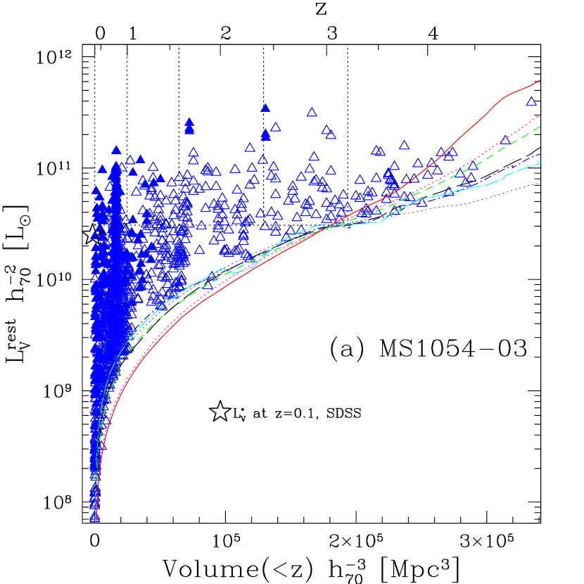
Figure 1.— The distribution of rest-frame $V$ luminosities as a function of enclosed co-moving volume and $z$ is shown for MS1054-03, the HDF-S, the HDF-N, and the CDF-S in figures (a), (b), (c), and (d) respectively for galaxies with $K_{s}^{\rm tot}$$<22.34$, $K_{s}^{\rm tot}$$<23.14$, $H_{160}^{\rm tot}$(AB)$<26.5$, and $K_{s}^{\rm tot}$$<21.34$. Galaxies which have spectroscopic redshifts are represented by solid points and for these objects ${\rm L^{rest}_{\lambda}}$ is measured at $z_{spec}$. The large star in each panel indicate the value of ${\rm L}^{\star}_{\rm local}$ from Blanton et al. (2003b). The tracks represent the values of ${\rm L^{rest}_{\lambda}}$ for seven template spectra normalized at each redshift to the limiting magnitude in that field. The specific tracks correspond to the E (solid), Sbc (dot), Scd (short dash), Im (long dash), SB1 (dot–short dash), SB2 (dot–long dash), and 10my (dot) templates. The horizontal dotted line each panel indicates the luminosity threshold ${\rm L}_{V}^{\rm thresh}$ above which we measure the rest-frame luminosity density $j^{\rm rest}_{\lambda}$ and the vertical dotted lines in each panel mark the redshift boundaries of the regions for which we measure $j^{\rm rest}_{\lambda}$.

3.2.1 Construction of Low Redshift Comparison Samples

All deep surveys are limited by a small volume at $z\lesssim 1$, e.g. even the GOODS CDF-S field encloses only $6.6\times 10^{4}{\rm Mpc}^{3}$ or a cube of $40$Mpc on a side, 50% of the distance to the Coma cluster. To build up a large volume at low redshift it is necessary to include a large redshift range in a single bin, which at low redshift smears together large epochs of time. To supplement our data at these low redshifts we utilized data from the COMBO-17 survey and from SDSS.

We computed $j^{\rm rest}_{\lambda}$ at $z<0.2$ for the SDSS Early Data Release (EDR; Stoughton et al. 2002) as in R03, deriving $j^{\rm rest}_{\lambda}$ in $UBVRI$ from maps of number density as a function of ${\rm L^{rest}_{\lambda}}$ and rest-frame color. These maps were computed as described in Blanton et al. (2003a). While the Poisson errors in the SDSS are negligible, cosmic variance and systematic errors do contribute to the uncertainties. For a more conservative error estimate, we adopt 10% errors on the luminosity density. For the SDSS luminosity function, our ${\rm L}_{V}^{\rm thresh}$ encompasses 28% of the total light.

To provide data at $0.2<z<0.9$ we used $j^{\rm rest}_{\lambda}$ measurements from the COMBO-17 survey (Wolf et al., 2003), which has a $\sim 30$ times larger survey area than the four deep fields combined. Specifically we used a catalog with redshifts of 29471 galaxies at $z<0.9$, of which 7441 had ${\rm L}_{v}^{rest}$$>$${\rm L}_{V}^{\rm thresh}$ . Using this catalog we calculated $j^{\rm rest}_{\lambda}$ identically to the deep fields. We divided the data into redshift bins of $\Delta z=0.2$ and counted the light from all galaxies contained within each bin which had ${\rm L}_{v}^{rest}$$>$${\rm L}_{V}^{\rm thresh}$. The size of the redshift slices was chosen to well sample the $0.2<z<1$ redshift interval while still being large enough to include many sources in each bin. The large solid angle of the COMBO-17 survey (0.75 deg²) assured that these slices still contained considerable co-moving volume. The formal 68% confidence limits were calculated via a bootstrapping method as in § 3.2. In addition, in Figure 2 we indicate the rms field-to-field variations among the three COMBO-17 fields. As also pointed out in Wolf et al. (2003), the field-to-field variations dominate the error in the COMBO-17 $j^{\rm rest}_{\lambda}$ determinations.

4. Results

In this section we first present our estimates of $j^{\rm rest}_{\rm V}$ and of the evolution of the volume averaged color of luminous galaxies. We then discuss the color evolution in terms of simple models. We also present the full rest-frame UV to optical volume averaged SED of luminous galaxies and show its evolution to higher redshifts, highlighting the mean SEDs of different subpopulations. Finally, we fit these mean SEDs with models and use the results to constrain the evolution in the global ${\cal M_{\star}}/{\rm L}$ and $\rho_{\star}$, also highlighting the contribution to the mass budget by different galaxy subpopulations.

4.1. The Luminosity Density

R01 were the first to estimate the evolution of the rest-frame optical luminosity function and luminosity density to $z\sim 3$, based on the number of rest-frame optically luminous galaxies in the HDF-S. In Figure 2 we show $j^{\rm rest}_{\rm V}$, $j^{\rm rest}_{\rm B}$, and $j^{\rm rest}_{\rm U}$ as a function of cosmic epoch for our four deep fields and for the complementary $z<1$ surveys. These estimates are given in Table 1 and Table 2 . As in R03, there is little evolution of $j^{\rm rest}_{\rm V}$ at $z<3$. Figure 2 also shows the large field-to-field variations present in our four deep fields. Large variations in $j^{\rm rest}_{\rm V}$ among the three COMBO-17 fields are also seen, as indicated by the dotted error bars in Figure 2. Still, it is encouraging that the mean evolution in $j^{\rm rest}_{\rm V}$ is smoother than in the individual fields, indicating that we are getting closer to a measure of the true volume average value.

The power of the COMBO-17 data is demonstrated here. With its inclusion it is apparent that there is a slight evolution toward brighter $j^{\rm rest}_{\rm V}$ out to $z\sim 1$, as found by many authors (e.g. Lilly et al. 1996; Wolf et al. 2003). Moving to bluer wavelengths the evolution from $z\sim 3$ to $z\sim 0$ becomes more apparent, even within our own data. This already foreshadows the trends with color that we discuss in the following section.

The field-to-field rms in $j^{\rm rest}_{\rm V}$ ranges from $20-75\%$ in our 4 redshift bins. From this it is clear that data must be combined over large areas to robustly measure the evolution, especially for bright galaxies, which may be strongly clustered (e.g. Giavalisco & Dickinson 2001; Daddi et al. 2003). To mitigate field-to-field variations the most it is desirable for the individual fields to be larger than the typical clustering scale of objects in the field or to be spread over many independent lines of sight (Somerville et al., 2004).

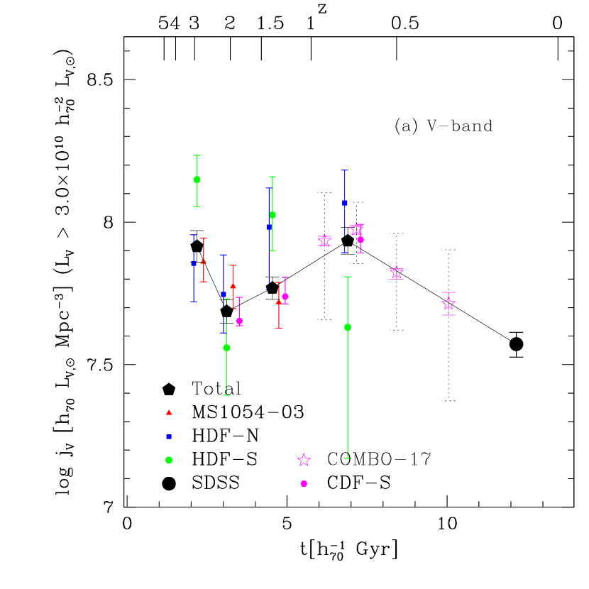
Figure 2.— The evolution of $j^{\rm rest}_{\rm V}$, $j^{\rm rest}_{\rm B}$, and $j^{\rm rest}_{\rm U}$ with time in panels (a), (b), and (c) respectively for galaxies with ${\rm L}_{V}^{rest}$$>$${\rm L}_{V}^{\rm thresh}$. The solid symbols indicate the values for the individual fields as labeled while the large solid symbol is the mean value. The values are offset in time for viewing clarity. The errorbars reflect the 68% uncertanties in each field as characterized by a bootstrap simulation. The dotted errorbars represent the explicit rms field-to-field variations among our four fields. The open stars are the values for the COMBO-17 data and the open circle is the value for the SDSS. The dotted errorbars in the COMBO-17 data reflect the field-to-field rms uncertainties among the 3 COMBO-17 fields. Note the large field-to-field variation even between fields as large as 0.25 square degrees. Note also that the MS1054-03 field was excluded from the lowest redshift bin because of the presence of a rich cluster and that we excluded the CDF-S from the highest redshift bin due to the depth of the NIR data in that field, which which made us highly incomplete at ${\rm L}_{V}^{rest}$$>$${\rm L}_{V}^{\rm thresh}$ and $z>2.41$.

4.2. The Volume Averaged Color and SED

We now proceed to measure the galaxy-averaged rest-frame colors at a given redshift/epoch. As discussed in R03 this average reflects a relatively smooth SFH for the ensemble of galaxies, even if individual SFHs are bursty. Therefore, a conversion of rest-frame color into a mean ${\cal M_{\star}}/{\rm L}$ will be more robust when modeling with a smooth SFH. In Figure 3 we illustrate this using an example which shows that the volume averaged color of a set of bursts behaves just like a population with the sum of their SFHs.

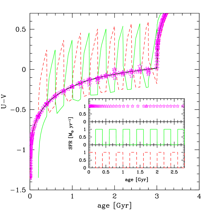
Figure 3.— A stylized example of how the volume averaged color of bursty SFHs reflects the sum of the individual SFHs. In the inset plot we show in the two lower panels two periodic SFHs with an identical duty cycle and peak SFR but which are perfectly out of phase. In the top panel we show the sum of their SFHs, which is equal to a constant. The main plot shows the evolution of the $(U-V)$ colors associated with the individual SFHs and the evolution of a constant SFR model which is simply the sum of the individual SFHs (thick black line). We also show the $(U-V)$ color which is derived from adding up the luminosities of each SFH in each band and using them to derive a total color as described in the text (stars). This luminosity weighted color is exactly the same as the color of a constant star formation model which is the sum of the individual SFHs.

In Figure 4 we present the redshift evolution of the luminosity weighted average color of all galaxies with ${\rm L}_{V}^{rest}$ $>3\times 10^{10}$${\rm~{}h_{70}^{-2}~{}L_{\odot}}$, computed using Equation 1. The colors become continuously redder from $\sim 3$ to $z\sim 0$.

Contrary to the conclusions of R03, with our multiple fields it is apparent that the colors are only slightly less susceptible to field-to-field variations than the luminosities, with the rms variations per redshift bin ranging from 5-50% for $(U-V)_{rest}$ and 20-75% for the $j^{\rm rest}_{\rm V}$. This indicates that the mix of SED types also varies greatly from field to field, implying that large area surveys are even necessary to study the mean stellar populations of luminous galaxies in the Universe.

In Figure 5 we show our average color estimates and those from COMBO-17 and SDSS in color-color space. It is clear that all of the average estimates lie on a narrow locus in this space. To interpret this trend we refer to Larson & Tinsley (1978) who demonstrated that individual galaxies with normal morphological types lie on a narrow locus in the $(U-B)_{rest}$ vs. $(B-V)_{rest}$ diagram and that galaxies with large bursts of star formation scattered away from the relation, preferentially to blue $(U-B)_{rest}$ colors. To ascertain the amount of “burstiness” in our average colors we therefore compare them to those of individual local galaxies from the NFGS (Jansen et al. 2000a) in Figure 5. In general our colors and those of COMBO-17 are similar to the colors of local galaxies, implying a relatively smooth ensemble SFH. Our data in the highest redshift bin, however, have a slight systematic offset to bluer $(U-B)_{rest}$ colors at a given $(B-V)_{rest}$ color with respect to the local sample. We explored whether part of this offset could result from systematic errors in the photometric redshifts. At $z>2$ it appears that $z_{phot}$ slightly overestimates the redshift on average, by about 0.2. These uncertainties likely result from an imperfect template set or an incorrect amount of extinction. Although the redshift solution is driven primarily by the rough position of the dominant break in the SED, small color mismatches in the template set can slightly change the redshift. These systematic redshift errors can indeed produce $(U-B)_{rest}$ colors which are bluer than the true values by up to 0.1 magnitudes, although they can’t entirely make up the differences with respect to the local data. The $(U-B)_{rest}$ color is especially sensitive to these effects, implying that more information than simply one color should be used to infer physical properties of the stellar population. The remaining differences between the high redshift and local samples can be understood, at least qualitatively, by considering the effects of bursty SFHs on the mean color. Although the deviation from a smooth SFH is reduced when averaging over more galaxies there is still some residual burstiness left.

We can also use the rest-frame UV to optical volume averaged SED to further constrain the nature of the mean stellar population. In Figure 6 we show the galaxy-averaged SED from the rest-frame UV through the optical for our four redshift bins and compare it to the SEDs of local galaxy templates. The volume averaged SED at all redshifts falls well within the locus of normal local galaxies. Even in our highest redshift bin the mean SED is not as blue as a local starburst. Also evident is the presence of a break in the mean SED between the $U$ and $B$ bands. That this break is present even in our highest redshift bin indicates that the rest-frame optical light at $z>1.6$ in rest-frame optically bright galaxies has significant contributions from evolved stellar populations.

In Figure 7 we also split our sample into DRGs and non-DRGs and display their volume averaged SEDs. This is only done in the two highest redshift bins, covering the redshift interval targeted, by design, by the DRG selection criterion. The DRG mean SED is uniformly redder than that of the non-DRGs. This is not surprising at rest-frame optical wavelengths since these galaxies were in fact selected to have red rest-frame optical (observed NIR) colors. The origin of the redder optical colors is partially elucidated by the detailed shape of the mean SED. It is apparent that the DRGs have stronger rest-frame optical breaks than the non-DRGs, indicative that evolved stellar populations are more prevalent in DRGs than in non-DRGs, to the same rest-frame optical luminosity limit. Similar conclusions were reached by Förster Schreiber et al. (2004) and L03 based on the results of SED fits to individual galaxies. DRGs, selected by their red rest-frame optical colors also have red UV SEDs.

In summary, it appears in all cases that the volume averaged SED of all rest-frame optically luminous galaxies has a strong contribution from evolved stellar populations and evolves to redder colors toward lower redshifts.

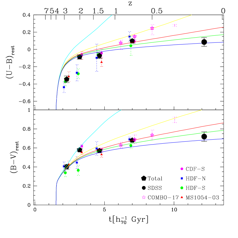
Figure 4.— The redshift evolution of the volume averaged $(U-B)_{rest}$ and $(B-V)_{rest}$. The symbols are identical to those in Figure 2 with the addition that the $(U-B)_{rest}$ colors have also been corrected for probable emission line contamination as in R03. For clarity we have also plotted the errorbars of the individual fields as dotted lines. The colors of the lowest redshift COMBO-17 point are artificially red due to the use of small central apertures to measure the color. For this reason we de-emphasize this point by only plotting a dotted errorbar. The integrated colors evolve redward with decreasing redshift with a much smoother progression than seen in the evolution of $j^{\rm rest}_{\rm V}$ in Figure 2. The solid tracks indicate a set of solar metallicity exponentially declining SFHs with $z_{form}=4$, $E(B-V)=0.25$ (using a Calzetti et al. 2000 attenuation law), and with timescales of 1, 3, 6, 10, and 100 Gyr moving from top to bottom. Although these are merely example SFHs they highlight the inability of simple models with an exponential SFH, dust content, and metallicity to fit the time evolution of the global colors.

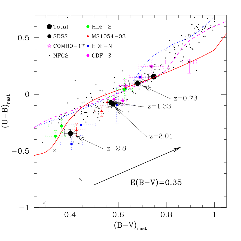
Figure 5.— The $(U-B)_{rest}$ vs. $(B-V)_{rest}$ at $z=$0.73, 1.33, 2.01, and 2.8 of all the stars in galaxies with ${\rm L}_{V}^{rest}$$>3\times 10^{10}$${\rm~{}h_{70}^{-2}~{}L_{\odot}}$. The large symbols are identical to those in Figure 4. For clarity we have plotted the errorbars of the individual fields as dotted lines and we do not plot the field-to-field errorbars for the COMBO-17 data. The small solid points are the colors of nearby galaxies from the NFGS (Jansen et al., 2000a), which have been corrected for emission lines. The small crosses are the NFGS galaxies which harbor Active Galactic Nuclei. The thin tracks correspond to an exponentially declining SFH with a timescale of 6 Gyr. The tracks were created using a Salpeter (1955) IMF and the BC03 models. The dotted track has no extinction, the dashed track has been reddened by $E(B-V)=0.15$, and the thin solid track has been reddened by $E(B-V)=0.35$, using the Calzetti et al. (2000) extinction law. The thick black arrow indicates the reddening vector applied to the solid model track. The emission line corrected data lie very close the track defined by observations of local galaxies but are systematically bluer than all of the smooth models.

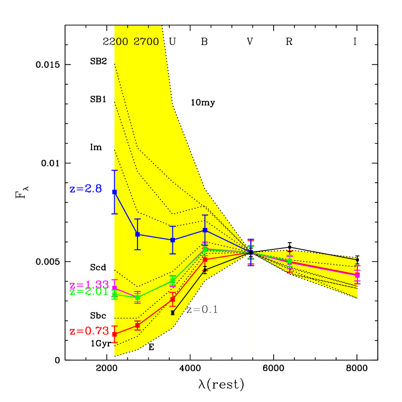
Figure 6.— The 2200${\rm\AA}$ through $I$-band volume averaged SED of all the galaxies with ${\rm L}_{V}^{rest}$ $>3\times 10^{10}$${\rm~{}h_{70}^{-2}~{}L_{\odot}}$. The different colored lines correspond to the different redshifts. The mean SEDs have been normalized to the same $V$-band rest-frame luminosity to highlight the evolution in the colors. The dotted lines are the SEDs of a set of galaxy templates, as labeled on the left side. The 2200${\rm\AA}$ through $I$-band volume averaged SED at all redshifts falls well within the range of colors occupied by “normal” nearby galaxies. Even at the highest redshift bin the mean SED looks more like that of a late type galaxy than of a starburst. A break is also visible between the $U$ and $B$ bands, indicating the presence of an evolved population - with an associated 4000${\rm\AA}$/Balmer break - that is dominating the light.

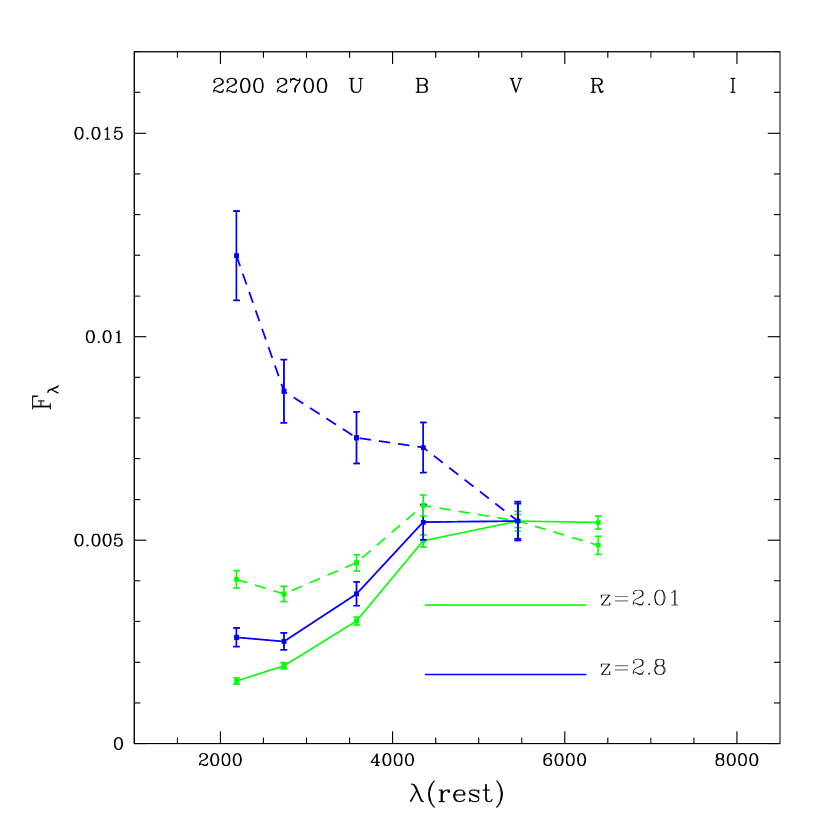
Figure 7.— Same as for Figure 6 but splitting the two highest redshift bins split into DRGs (solid lines) and non-DRGs (dashed lines). At both redshifts the DRGs are redder than the non-DRGs, both in the rest-frame optical - where breaks are easily visible - and in the rest-frame UV. Because the DRGs still have light in the rest-frame UV the red colors are likely caused by a mix of old stars and dusty star formation.

4.3. Modeling the Volume Averaged Stellar Population

In order to derive global ${\cal M_{\star}}/{\rm L}$ and subsequently $\rho_{\star}$ values from our mean SEDs it is necessary to use models to interpret them. In R03 we derived ${\cal M_{\star}}/{\rm L}_{V}$ estimates by using exponentially declining models applied to the global $(U-V)_{rest}$ color in which the SFR timescale, dust content, and metallicity were constant as a function of redshift . With better data we attempt this same exercise again and find that the same simple models cannot accurately describe our higher precision data. We show five example models in Figure 4. These models have a Salpeter (1955) IMF, solar metallicity, $E(B-V)=0.25$, $z_{form}=4$ and exponentially declining SFHs with timescales of 1, 3, 6, 10, and 100 Gyr. Although these models represent only one possible set of parameters we find it is generally impossible to simultaneously fit the $(U-B)_{rest}$ and $(B-V)_{rest}$ colors, in the sense that the models have consistently too red $(U-B)_{rest}$ colors for a given $(B-V)_{rest}$ color for our data but with the opposite trend apparent for the COMBO-17 data. This same disagreement is seen in Figure 5 where we plot our data, along with that of COMBO-17 and SDSS, in the $(U-B)_{rest}$ vs $(B-V)_{rest}$ color plane. The emission line corrections we applied to the colors did move the data in the direction of better agreement with the models but these corrections are already quite extreme at high redshift (0.04 magnitudes in $(U-B)_{rest}$) and larger shifts would be difficult to accommodate given the range in corrections inferred from the NFGS. To determine the robustness of the disagreement between the models and data we have explored different combinations of metallicity and extinction values and have found that no single set can reproduce these two colors at all redshifts. As we have mentioned already, however, the $(U-B)_{rest}$ color in particular is susceptible to redshift uncertainties and uncertainties in the emission line corrections.

To mitigate the influence of one color on the global fit we choose to model the full UV-optical volume averaged SED to constrain the set of population parameters. As we have pointed out earlier, averaging over the whole galaxy population also averages over the SFHs of the individual galaxies, making it more appropriate to apply smoothly varying SFHs when performing the model fits. This point of view is generally supported by the general agreement of our mean SEDs with those of “normal” local galaxies, which have been shown to be consistent with extended, relatively smooth SFHs (e.g. Kennicutt, Tamblyn, & Congdon 1994). With our choice of simple models there are four possible free parameters that we consider: age, metallicity, dust, and SFH. We use the BC03 models and an updated version of the Hyperz code (Bolzonella et al., 2000) to fit our data (Bolzonella private communication). We assume a Salpeter IMF with lower and upper mass cutoffs of 0.1 and 100 ${\cal M_{\odot}}$ respectively. Fitting with a different IMF, e.g. a Chabrier, would result in a scaling of the ${\cal M_{\star}}/{\rm L}$ values by a constant factor at all redshifts (assuming that the IMF is universal). Thus the relative trends would be preserved. In all cases we use the Calzetti et al. (2000) attenuation law. We find that there exists some combination of parameters that can fit the rest-frame UV-optical volume averaged SEDs as long as we don’t require that the model parameters are the same at all redshifts.

When fitting broad band photometry, especially only out to the rest-frame optical, there are very large degeneracies between age, SFH, metallicity, and dust content, e.g. P01, Shapley et al. (2001). For example, in some cases high redshift SEDs can be fit reasonably well with both a constant SFH (hereafter CSF), moderate ages, and high extinctions and SFRs, or with an exponentially declining model with lower extinction and SFRs. Despite these degeneracies, however, ${\cal M_{\star}}/{\rm L}$ are better constrained, since different combinations of stellar population parameters can give similar derived mass-to-light ratios (Förster Schreiber et al., 2004; van Dokkum et al., 2004). We will therefore use our fits to measure ${\cal M_{\star}}/{\rm L}$ but will not discuss the constraints on the stellar population parameters in detail. There is tentative evidence from NIR spectroscopy of bright galaxies at $z<3$ that metallicities are typically around solar (van Dokkum et al., 2004; Shapley et al., 2004; de Mello et al., 2004) and we therefore limit our fits to solar metallicity.

To span the range of possible models we perform fits with either a CSF, Simple Stellar Population (SSP), or exponentially declining model with a timescale of 300 Myr ($\tau_{\rm 300Myr}$). In all cases we restrict the age of the population in each redshift bin to be younger than the age of the Universe for the middle redshift in that bin. We parameterize the amount of extinction by the magnitudes of attenuation in the $V$-band $A_{V}$. For the CSF and $\tau_{\rm 300Myr}$ models we allow the extinction to vary between $0<A_{V}<3.0$ and for the SSP models between $0<A_{V}<0.5$. This latter choice is to prevent the fitting from choosing highly extincted very young models with no ongoing star formation, which would result in unphysically large intrinsic luminosities. The upper limit of 3.0 magnitudes of extinction does not affect our conclusions. For each redshift bin we choose the best-fit SFH, age, and extinction combination and use the ${\cal M_{\star}}/{\rm L}_{V}$ of that model, which includes the stellar mass loss from evolved stars. We then multiply that ${\cal M_{\star}}/{\rm L}_{V}$ by $j^{\rm rest}_{\rm V}$ to derive $\rho_{\star}$.

To derive uncertainties on ${\cal M_{\star}}/{\rm L}_{V}$ and $\rho_{\star}$ we fit the ensemble of mean SEDs produced by our bootstrap simulation described in § 3.2. Each bootstrapped SED was computed from the same set of galaxies, which is necessary because each galaxy contributes luminosity in every passband, i.e. the $j^{\rm rest}_{\lambda}$ values are correlated. We then use the distribution of ${\cal M_{\star}}/{\rm L}_{V}$ and $\rho_{\star}$ values from the fit to the ensemble of SEDs and determine the 68% confidence limits.

The best fit SFH for each volume averaged SED is presented in Figure 8. We also indicate the formal best fit SFH, which is the $\tau_{\rm 300Myr}$ model for the three lowest redshift bins and the SSP model for the highest redshift bin. It is important to note, however, that the $\tau_{\rm 300Myr}$ model is statistically allowed at all redshifts and that our ${\cal M_{\star}}/{\rm L}$ determinations are not very sensitive to the exact SFH. As was visible in Figure 6 the rest-frame optical break is present at all redshifts, with the strength of the break decreasing toward higher redshifts. This is also reflected in the model fits.

We also fit the mean SED from the SDSS survey to constrain the evolution of ${\cal M_{\star}}/{\rm L}$ and $\rho_{\star}$ to low redshift. The COMBO-17 data were very useful for characterizing the overall trends of color and for assessing the applicability of certain models for the color evolution. Nonetheless, we do not model the COMBO-17 data in detail since the lack of deep NIR observations limits us to only a relatively small range in rest-frame wavelength at each redshift, with correspondingly poor constraints on the best-fit ${\cal M_{\star}}/{\rm L}_{V}$. The low redshift sample from the SDSS is crucial as our ${\rm L}_{V}^{rest}$ cut complicates the use of literature values for $\rho_{\star}$, which are always quoted as total values. By fitting the mean SED of the local sample as determined with our ${\rm L}_{V}^{rest}$ threshold we can consistently track the evolution over redshift. The only differences in analyzing the low and high redshift samples is in the allowed stellar population parameters and the derivation of uncertainties. Because luminous galaxies from the SDSS are almost entirely made up of evolved early type populations (Blanton et al., 2003a; Kauffmann et al., 2003) we limited the attenuation to 1 magnitude in the $V$-band. In addition it is difficult to obtain a realistic uncertainty estimate for the SDSS. The uncertainties in $j^{\rm rest}_{\lambda}$, and hence in ${\cal M_{\star}}/{\rm L}$ and $\rho_{\star}$ are dominated by systematic uncertainties. Therefore we give a 10% error to all derived SDSS quantities.

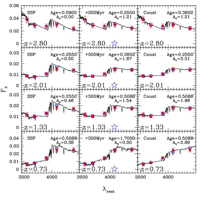
Figure 8.— The best fit models to the volume averaged SED. Each row corresponds to one of the redshift bins and each column corresponds a different SFH. The panel in each row with a star indicates the formal best fit SFH, although the other SFHs are generally allowed within the uncertainties. The filled points show the measured values and the open circles show the best fit model fluxes. As in Figure 6 the rest-frame optical break of both the data and best-fit model is apparent at all redshifts and increases toward lower redshifts.

4.4. ${\cal M_{\star}}/{\rm L}_{V}$ and $\rho_{\star}$

In Figure 9 we show the evolution of the derived $\langle{\cal M_{\star}}/{\rm L}_{V}\rangle$ for luminous galaxies as a function of time and redshift. These are also given in Table 4. As expected the bluer colors of the volume averaged SEDs and the decrease in the break strength toward higher redshift implies a lower value of $\langle{\cal M_{\star}}/{\rm L}_{V}\rangle$. $\langle{\cal M_{\star}}/{\rm L}_{V}\rangle$ increases by a factor of $\sim 10.7$ from $z=2.8$ to $z=0.1$.

Using the $\langle{\cal M_{\star}}/{\rm L}_{V}\rangle$ values and the $j^{\rm rest}_{\rm V}$ measurements we derive $\rho_{\star}$ for galaxies at high redshift and in the SDSS with ${\rm L}_{V}^{rest}$$>$${\rm L}_{V}^{\rm thresh}$. Our absolute $\rho_{\star}$ measurements at $0<z<3.2$ are given in Table 3. The mass density in luminous galaxies between decreases by a factor of $\approx 4.8$ between $z=0.1$ and $z=2.8$ and $\sim 50\%$ of the stellar mass was in place by $z\gtrsim 1$. This is in broad agreement with the results of R03, who measured a decline by a factor of $\sim 10$ in $\rho_{\star}$ between $z=0.1$ and $z=2.8$, although with significantly larger errorbars and with no accounting for cosmic variance. The rms field-to-field variations in $\rho_{\star}$ among our four fields ranges from $40-61\%$.

To compare our data to that from other authors we scale our data to “total” values. We calculate an upwards correction factor of 2.1 by measuring the total SDSS $\rho_{\star}$ value and comparing it to $\rho_{\star}$ for the SDSS galaxies with ${\rm L}_{V}^{rest}$$>$${\rm L}_{V}^{\rm thresh}$. After correcting all our measurements to total we normalize our values to the $z=0$ $\rho_{\star}$ measurement of C01 and plot them along with those of other authors in Figure 10. The relative values are given in Table 5. We also determine how the inferred evolution in the total $\rho_{\star}$ changes if we allow ${\rm L}_{V}^{\rm thresh}$ to evolve in the same way as our ${\cal M_{\star}}/{\rm L}_{V}$ values. The change this can induce is indicated by the vertical extent of the boxes in Figure 10 and is reflected in the confidence interval in $\Delta\rho_{\star}$ given in Table 5. Our local total mass density measurement from SDSS is $\approx 25\%$ lower than that of C01. Some of this discrepancy may be due to the slightly higher mean redshift of our data. C01 estimate their stellar masses at $z=0$ whereas the mean redshift for the SDSS sample is 0.1. Using the $z=0.1$ SFRD from Brinchmann et al. (2004) we would predict that $\rho_{\star}$ would increase by $\approx 9\%$ between $z=0.1$ and 0, accounting for some of the discrepancy. Another possible source of the discrepancy is the use by C01 of a fixed formation redshift of $z=20$ for their SED fitting derived $\cal{M_{\star}}$ estimates.

According to Bell et al. (2003) the old age assumed for all galaxies could bias their estimates by $\approx 10\%$ Bell et al. (2003). By refitting the SEDs of galaxies with SDSS and 2MASS data and letting the age vary Fontana et al. (2004) estimated that forcing an old age can bias the masses from C01 upwards by $<20\%$. Taking all these effects into account, the remaining difference between our SDSS point and that of C01 falls well within the range of expected systematic errors in our $\rho_{\star}$ estimates.

Compared to the C01 point, the mass density at $z=2.8$ is 5–8 times less than at $z=0$, where the range corresponds to our formal 68% confidence limits for a fixed ${\rm L}_{V}^{\rm thresh}$. As discussed in §4.5, however, it may not be appropriate to compare the evolution of our ${\rm L}_{V}^{rest}$ limited sample to that of the total estimates presented by different authors (see below). If we instead allow ${\rm L}_{V}^{\rm thresh}$ to vary along with our ${\cal M_{\star}}/{\rm L}_{V}$ values the mass density at $z=2.8$ is constrained to be 5.3–16.7 times less than at $z=0$.

At higher redshifts $\rho_{\star}$ is estimated by other authors using SED fits of individual galaxies. In all cases we have converted to a Salpeter IMF when necessary. Brinchmann & Ellis (2000) fit a set of $I$-band selected galaxies at $z<1$ from the Canada France Redshift Survey (CFRS). They are only complete over the range $10.5<{\rm log}{\cal M_{\star}}<11.6$ and their value here includes a $20\%$ correction to a total mass density recommended by Brinchmann & Ellis (2000). Drory et al. (2004) estimate $\cal{M_{\star}}$ for $z<1.2$ galaxies with $K<19$ over 0.28 deg² from the Munich Infrared Cluster Survey (MUNICS). They also adopt an SED fitting technique but use their best-fit models to derive ${\cal M_{\star}}/{\rm L}_{K}$ and then extrapolate their SEDs from the observed to the rest-frame $K$-band to derive ${\rm L}_{K}^{rest}$. Using the DEEP2 spectroscopic survey coupled with $K$-band imaging, Bundy et al. (2006) use an SED fitting technique to estimate galaxy masses and then fit a Schechter function and extrapolate it to get their $\rho_{\star}$ estimates. At high redshifts/faint magnitudes, they supplemented their spectroscopy with photometric redshifts but these have a minimal effect on the derived $\rho_{\star}$ values. The errorbars for the Bundy et al. (2006) points are from the variance in $\rho_{\star}$ between their four fields. Borch et al. (2006) computed the stellar mass density from 25,000 galaxies in the COMBO-17 survey. They fit their combination of 17 broad and medium optical bandpasses with SEDs to derive the stellar masses for each galaxy. They then fit Schechter functions to their data in each redshift bin and integrate this to derive $\rho_{\star}$. Fontana et al. (2004) use the K20 survey to measure the stellar mass function out to $z=2$ using stellar masses derived by SED fitting of individual galaxies. They then integrate this mass function to obtain $\rho_{\star}$. In their $1.5<z<2$ bin their mass function is complete only down to the $\sim{\cal M^{\star}}$ value of their best-Schechter fit to the mass function and the extrapolation to lower $\cal{M_{\star}}$ is large and uncertain. D03 and F03 derive $\rho_{\star}$ at $z\sim 3$ from the HDF-S and HDF-N WFPC2 fields respectively, where the raw data in the HDF-S are in common with the FIRES data and where the HDF-N catalog is identical to what is used in this paper. The techniques in both these papers are nearly identical, using SED fitting of individual galaxies to determine the mean ${\cal M_{\star}}/{\rm L}$ for all galaxies and then applying this to the luminosity density as determined by integrating a Schechter function fit to the rest-frame optical luminosities. Drory et al. (2005) estimate the mass density in the FORS Deep Field (FDF) using an $I$-band selection sample and in the GOODS-S field using a $K$-band selected sample drawn from the same raw data as used for this paper. They derive mass densities by fitting the observed SEDs and then add up all the galaxies in their sample at each redshift. Although they measure $\rho_{\star}$ out to $z\sim 5$ we only plot it out to $z\sim 2$ for two reasons. First, their $I$-band selection in the FDF corresponds to a selection in the UV at $z<1.5$ and the authors are therefore more sensitive to unobscured star formation than to stellar mass. They point out that their $I$-band data is deep enough to detect all but 10% of the $K$-selected objects in the deep FIRES images of the HDF-S but it is exactly these missed objects which comprise a significant fraction of the mass density at high redshift, i.e. DRGs. Second, although they do have $K$-band data in the GOODS-S field it is not deep enough to be mass complete for any but the most massive objects at $z>2$, but they add up all objects, regardless of whether they are complete for those masses. It is therefore difficult to interpret their total values at $z>2$. Glazebrook et al. (2004) determine stellar masses by fitting the observed SEDs with stellar population synthesis models and then compute $\rho_{\star}$ using a $V/V_{max}$ method. The compute $\rho_{\star}$ down to different mass limits and note their decreasing incompleteness in mass with increasing redshift and decreasing mass. After converting to a Salpeter IMF we plot their points down to their lowest mass limit, $10^{10.45}$${\cal M_{\odot}}$. At the highest redshift bins they are incomplete and the resultant $\rho_{\star}$ values can only be considered as lower limits.

In our $0<z<1.0$ redshift bin our data fall slightly lower than the other determinations. This difference may be because the CDF-S is underdense at low redshifts. We suspect this because Wolf et al. (2003) note that the Extended CDF-S is underdense at $0.2<z<0.4$ and that this trend apparently is true at $z\lesssim 0.6$ (Papovich private communication). Although there is a loose structure in the Extended CDF-S at $z=0.67$ and a cluster at $z=0.73$ Gilli et al. (2003), these should not dominate the counts over the much larger CDF-S field. We don’t include the MS1054 data in our $0<z<1$ measurement because of the massive cluster in that field. However, the large field-to-field variation among our 4 fields at $z<1$ makes our data consistent with those from other surveys. At $z>1$ our $\rho_{\star}$ estimates agree very well with those of the other authors but with smaller formal errors corresponding to the lower uncertainties afforded by the multiple fields. The only notable discrepancy is with the HDF-N determinations of D03; we address a possible cause for this in the following subsection.

We also show the curves that correspond to the integral of the parametric fit to the SFR($z$) curve from (Cole et al. 2001; C01), both with and without a substantial extinction correction. As pointed out by, e.g. D03, R03, F03, and Fontana et al. (2004), an extinction correction to the UV-derived star formation rates is required to match the $\rho_{\star}$ measurements at all redshifts, although the nature of this correction is highly uncertain. The $\rho_{\star}$ evolution predicted from the UV selected extinction corrected SFR is in broad agreement with the direct $\rho_{\star}$ measurements, notably at $z\sim 3$. Nonetheless, the measurements, including those from the literature are systematically below the extinction corrected curve by about 0.2-0.4 dex at $z<2$, with the exception of the Drory et al. (2004) data. This slight offset could be due to an erroneously high extinction correction to the SFR estimates, but these can’t be changed too much without coming into disagreement with the local $\rho_{\star}$ determinations. Additionally, some of the disagreement may come from systematic underestimates of $\rho_{\star}$, although it is not immediately clear what effects would plague all surveys, which use different techniques to estimate the mass densities. Finally, it may be that the galaxies which enter into the SFR($z$) determinations are too faint in the rest-frame optical to enter the NIR selected samples. The star formation rate density (SFRD) measurements rely on an extrapolation to the faint end of the rest-frame UV luminosity function. Estimates of the faint end slope have a large range, with the original determination from the HDF-N by Steidel et al. (1999) being $\approx-1.6$ but with a later measurement from the FORS Deep Field giving a value of $\approx-1.1$ (Gabasch et al., 2004). Also, as we describe in §4.5 the $\rho_{\star}$ measurements can have systematic errors at the factor of $\sim 2$ level which could also account for the difference. Obviously resolving the discrepancy between these two curves rests as much on an accurate determination of the SFR evolution as on that of $\rho_{\star}$.

4.4.1 The Stellar Mass Budget

With the larger number of galaxies afforded by our large area we can now split the sample into DRGs and non-DRGs to determine their relative contributions to the stellar mass budget. Using the mean SEDs for these two subsets we calculate ${\cal M_{\star}}/{\rm L}_{V}$, which is shown in Figure 9. The mean ${\cal M_{\star}}/{\rm L}_{V}$ for DRGs is a factor of 1.1 and 3.6 higher than for the non-DRGs at $z=2.01$ and 2.8 respectively. The higher ${\cal M_{\star}}/{\rm L}$ values for DRGs are in qualitative agreement with the results from SED fitting of individual galaxies (Förster Schreiber et al., 2004; van Dokkum et al., 2004; Labbé et al., 2005).

We show the corresponding mass densities as the blue and red filled pentagons in Figure 11. The DRGs contribute 30% and 64% of the stellar mass density at $z\sim 2$ and 2.8 respectively, comparable to that from UV selected samples. As shown in Franx et al. (2003) and more recently by Reddy et al. (2005) and (van Dokkum et al., 2006) DRGs are almost entirely absent in rest-frame UV selected samples like the LBG or BM/BX samples. Yet, they make up a comparable fraction of the mass budget down to similar rest-frame optical limits, showing that rest-frame UV selection misses significant amounts, if not most, of the stellar mass at $1.6<z<3.2$. Therefore NIR selection is crucial to obtaining a comprehensive and unbiased view of the high redshift Universe. The important contribution of DRGs agrees with new results from van Dokkum et al. (2006) who show that they are the most numerous constituent of the population of galaxies with $\cal{M_{\star}}$$>10^{11}$${\cal M_{\odot}}$ and $2<z<3$. It may be that the relatively unobscured star-forming UV-selected galaxies are over-represented in our luminosity selected sample due to their lower mass-to-light ratios. If this is true then the contribution of DRGs in a mass-selected sample should therefore be higher.

Interestingly the mass density of non-DRGs in our highest redshift bin is very similar to the HDF-N, which is $\sim 2$ times underdense compared to the total mass density from this work and from F03 and R03. This may indicate that much of the field-to-field variation at high redshift originates in the population of red massive galaxies. This was already indicated by the higher clustering amplitude of red galaxies seen by Daddi et al. (2003) in the HDF-S FIRES field and is also found by van Dokkum et al. (2006) who show that the CDF-S is underdense in massive ($\cal{M_{\star}}$$>10^{11}$${\cal M_{\odot}}$) galaxies at $2<z<3$. Clustering measurements of galaxies at high redshift as a function of color and over a much larger area will directly address this issue (Quadri et al. in preparation).

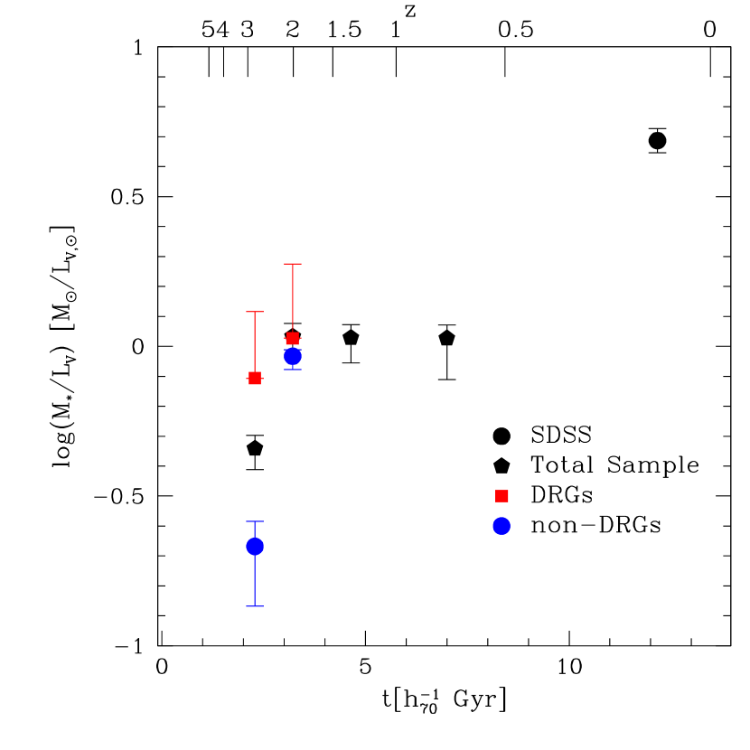
Figure 9.— The evolution of ${\cal M_{\star}}/{\rm L}_{V}$ for luminous galaxies with time and redshift, as derived by model fits to the volume averaged SEDS. The black pentagons are for the entire ${\rm L}_{V}^{rest}$$>$${\rm L}_{V}^{\rm thresh}$ sample and the blue circles and red squares are for non-DRGs and DRGs respectively. The open circle represents the local determination from the SDSS.

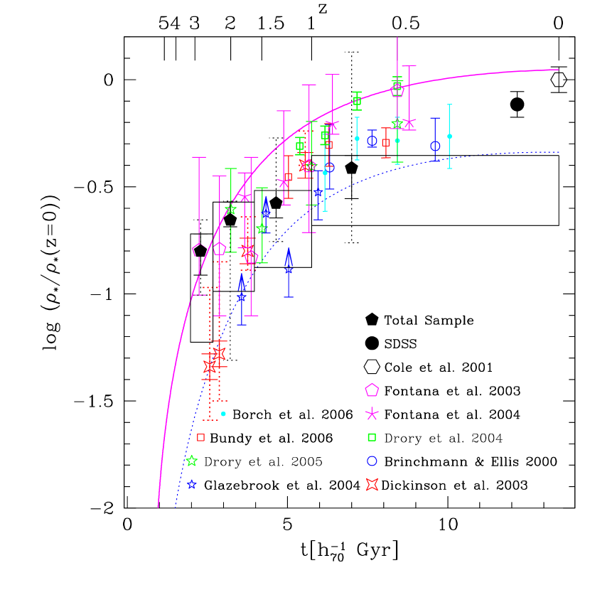
Figure 10.— The relative evolution of $\rho_{\star}$ with time and redshift. The symbols are as indicated in the plot. All quantities have been normalized to the local stellar mass density measured from Cole et al. (2001). As described in the text, most other authors have quoted “total” values determined by extrapolating fits to the luminous/massive galaxy population. Our measurements, on the other hand, are explicitly restricted to the luminous galaxy population, and are complete at ${\rm L}_{V}^{rest}$$>$${\rm L}_{V}^{\rm thresh}$. The dotted errorbars on the solid pentagons indicate the minimum and maximum $\rho_{\star}$ values among our fields and given an indication of the field-to-field variation. The horizontal extent of the solid boxes indicates the redshift range over which of our points are derived. The vertical extent of the solid boxes indicates the range in $\rho_{\star}$ values that are obtained by allowing the rest-frame luminosity threshold to evolve to fainter luminosities at lower redshifts in accordance with our derived evolution in ${\cal M_{\star}}/{\rm L}_{V}$. The mass density averaged over our four fields agrees well with most other surveys. The one notable exception is the HDF-N (D03) which has a substantially lower value than either the HDF-S or the mean value computed here. The two curves are the integrals of the Cole et al. (2001) parametric fit to the SFR($z$) data. The solid magenta line is the fit to the extinction corrected data and the dotted blue line line is for the data without an extinction correction. As has been noticed by many authors an extinction correction to the SFR($z$) measurements is necessary to reproduce the $\rho_{\star}$ measurements at almost all redshifts. There is a slight systematic difference between the $\rho_{\star}$ estimates and the integral of the SFR($z$) curve.

4.5. Possible Systematic Errors and Biases

There are various systematic errors which can affect our conclusions. First is the limitation that our observations only probe out to the rest-frame $V$-band in our highest redshift bin. While stellar mass-to-light ratios are much less variable in the rest-frame optical than the rest-frame UV they can still vary by an order of magnitude or more at a given ${\rm L}_{V}^{rest}$, depending on e.g. SFH, age, and extinction. Also, the extinction in very dusty starbursts can still be quite high in the rest-frame optical, implying that the light (and hence mass) from highly extincted stars will be missed. The work of Labbé et al. (2005) and Shapley et al. (2005) constrain the possible errors by deriving $\cal{M_{\star}}$ for objects using rest-frame NIR data obtained with the IRAC instrument on the Spitzer Space Telescope. For the most part $\cal{M_{\star}}$ derived from these fits agree with those derived from fitting only out to the rest-frame optical, although the $\cal{M_{\star}}$ uncertainties are reduced with the longer wavelength baseline. This implies that most of the stars that are visible in the rest-frame NIR are also visible in the optical, even though they may have a higher extinction. If significant stellar mass exists in environments which are obscured at optical and NIR wavelengths then our results would be biased. The amount of such heavily obscured stellar mass at $z<1$ is small, but increases rapidly out to higher redshift (Le Floc’h et al., 2005). If the fraction of extremely obscured stellar mass in rest-frame optically luminous objects at $z>1$ becomes significant then the decline in the true mass density will be shallower than what we observe.

Another systematic effect may stem from our relatively bright magnitude limits. Even in the HDF-S, which has the deepest $K_{s}$-band data in existence, we are limited to probing high luminosity galaxies and therefore may not be measuring a representative sample of the full galaxy population. We estimate the amount of light that we miss with our ${\rm L}_{V}^{rest}$ limit by using the rest-frame $B$-band luminosity function of Giallongo et al. (2005). We convert their Schechter parameters to the $V$-band by correcting ${\rm L}^{\star}$ using the mean $(B-V)_{rest}$ in each redshift bin. At $z=$0.73, 1.33, 2.01, and 2.8 our luminosity limit encompasses approximately 38, 40, 45, and 44% of the total $V$-band light respectively. We also check these numbers using the rest-frame $V$-band luminosity function from Marchesini et al. (2006) and find that our ${\rm L}_{V}^{rest}$ limit encompasses approximately 58 and 70% of the light in our two highest redshift bins. This is not to say that our relative trends in mass density will be more affected than other surveys that claim to measure “total” mass densities. Some of these surveys, e.g. D03 and F03, assume a faint end slope of the luminosity function as determined at lower redshift and use it to extrapolate their observed quantities to fainter levels. $\rho_{\star}$ is then derived by multiplying the resultant luminosity density by the mean ${\cal M_{\star}}/{\rm L}$ for their directly observed galaxies. While formally integrating over all luminosities, the implicit assumption about the constancy of the faint end of the luminosity function is largely uncertain. If the low end of the galaxy luminosity function is much steeper at high redshifts than at low redshifts this could cause the true decline rate in $\rho_{\star}$ to be less than what we observe. In addition, if rest-frame optically faint galaxies have very different ${\cal M_{\star}}/{\rm L}$ values than brighter ones a bias in the determinations will occur. The only solution to this quandary will be to go significantly deeper than the current deepest surveys in the $K$-band. Given the substantial investment in telescope time required to obtain the HDF-S FIRES data (100 hours) only space-based observation will be able to push to significantly fainter limits.

In R03 and in Figure 3 we demonstrated the advantages of averaging over the galaxy population when deriving stellar mass-to-light ratios. One possible complication may result when the different populations being averaged have very different extinction properties, such as the difference between LBGs and DRGs in our sample. We have explored the possible magnitude of such an error by fitting various combinations of models with SFHs and extinctions that correspond to star-forming DRGs, passive DRGs, and LBGs (e.g. P01; Shapley et al. 2001; Förster Schreiber et al. 2004; Labbé et al. 2005). Specifically we have used 3 models consisting of a 1 Gyr old CSF model with $A_{V}\sim 2$, a 2.9 Gyr old passive population with no extinction, and a 300 Myr old galaxy with $A_{V}\sim 0.6$. Depending on the exact contributions of the different populations to the mean SED errors of up to a factor of 2 in the derived masses can exist. We have also checked for the presence of these errors in our own data by using the DRG and non-DRG subsamples discussed in § 4.4.1. On average these two subsamples have very different stellar populations and extinctions (Förster Schreiber et al., 2004; van Dokkum et al., 2004; Labbé et al., 2005) but the sum of the $\rho_{\star}$ contributions from the two subsamples is within $15\%$ of the value measured for the total population, implying that this uncertainty is not dominant.

We also have explored the effect of our limited choice of SFH on our results. We increased the number of SFHs to include SSP, CSF, $\tau_{\rm 100Myr}$, $\tau_{\rm 300Myr}$, $\tau_{\rm 500Myr}$, $\tau_{\rm 800Myr}$, $\tau_{\rm 1Gyr}$, $\tau_{\rm 3Gyr}$, $\tau_{\rm 6Gyr}$, and a SFH that corresponds to the globally averaged SFR($z$) from Cole et al. (2001). With this larger range in SFHs the best-fit $\rho_{\star}$ values decrease by $<15\%$ and the confidence limits in $\rho_{\star}$ remain unchanged. Therefore our choice of SFH is not a large source of error.

Field-to-field variations are an obvious source of error, especially since the high luminosity galaxies we are examining are likely to be heavily clustered (Adelberger et al., 2004; Daddi et al., 2003). We have attempted to mitigate this as much as possible by using data from every available field where suitably deep optical and NIR data are available. Obviously deep NIR imaging over many spatially disjoint fields is crucial to making progress in this arena. This will require large investments of time on the next generation of wide-field NIR imagers on 8-meter class telescopes (e.g. HAWK-I/VLT, MOIRCS/Subaru).

The IMF is poorly constrained at high redshift. Although observations of the spectral signatures of massive stars in some LBGs indicate that the high mass slope must be close to Salpeter (Pettini et al., 2000) some authors have argued for the necessity of a top-heavy IMF at high redshift to explain abundance ratios in elliptical galaxies (e.g. Matteucci 1994 and Nagashima et al. 2005) and the abundance of submillimeter galaxies at $z\sim 2$ (Baugh et al., 2005). As noted in § 4.4 changing the lower end of the IMF would simply result in a scaling of all the $\rho_{\star}$ and SFR($z$) measurements by the same amount. A non-universal IMF, however, either as a function of time, environment, or metallicity would result in a biased determination of the evolution in $\rho_{\star}$ and SFR($z$).

In our modeling we assume solar metallicity and a Calzetti et al. (2000) attenuation law. It is impossible to constrain these directly using broad-band photometry. To determine the sensitivity to these assumptions we re-fit our data using $Z=0.004{\rm Z_{\odot}}$ models and found that $\rho_{\star}$ declines by $0.1-0.25$dex. This is somewhat less than the $0.3-0.5$dex change found by P01 and the reason is not entirely clear. It may be because our mean SEDs are significantly redder at all redshifts than the very blue starburst SEDs modeled by P01. We explore the dependence on the dust attenuation law by fitting using the SMC extinction curve of Prévot et al. (1984). In this case $\rho_{\star}$ decreases by $<0.1$dex. We conclude that uncertainties in the metallicity and dust extinction can result in up to a 0.2 dex error in our $\rho_{\star}$ estimates.

We rely entirely on BC03 models to interpret the average SEDs. van der Wel et al. (2006), however, have recently pointed out that the BC03 models incorrectly predict the evolution in ${\cal M_{\star}}/{\rm L}_{K}$ and rest-frame $B-K$ color for early type galaxies at $z<1$. The Maraston (2005) models do a better job at the fitting the evolution. In the rest-frame optical, the BC03 and the Maraston models yield identical ${\cal M_{\star}}/{\rm L}_{V}$ values for all models with $(U-V)_{rest}>0.5$ but the Maraston models yield ${\cal M_{\star}}/{\rm L}_{V}$ values between 5 and 35% higher for all models with $0<(U-V)_{rest}<0.5$ (for solar metallicity and a Salpeter IMF). Since our $(U-V)_{rest}$ colors range from $(U-V)_{rest}$$\approx 0$ at our highest redshift bin to $(U-V)_{rest}$$\approx 1$ at $z=0$, adopting the Maraston models would make our mass density evolution shallower by 5-35%. This is not a dominant source of uncertainty in our analysis.

Our analysis relies heavily on the use of photometric redshifts. An incorrect estimate of the redshift will lead to errors in the rest-frame colors and luminosities, and hence in the stellar masses. Unfortunately the most thorough calibrations for $z_{phot}$ estimates have only been performed for UV-bright populations for which abundant spectroscopic redshifts are already in hand. As we indicated in the previous section, however, much of the stellar mass density at high redshift likely resides in UV-faint objects, where $z_{phot}$ estimates are largely untested. Nonetheless, initial progress with optical and NIR spectroscopy of DRGs (Kriek et al. 2006; Wuyts et al. in preparation) has shown that the photometric redshifts for these objects, while slightly less reliable than for optically selected samples, are rarely catastrophically wrong. Looking at the whole spectroscopic sample with ${\rm L}_{V}^{rest}$$>$${\rm L}_{V}^{\rm thresh}$ we find that $z_{phot}$ errors result in systematic errors in ${\rm L}_{V}^{rest}$ of $\approx 4\%$ and $1\%$ at $z<1.5$ and $z\geq 1.5$ respectively. The systematic errors in $(U-V)_{rest}$ are also small, $\approx 5\%$ and $11\%$, at $z<1.5$ and $z\geq 1.5$ respectively. With the caveat that the spectroscopic samples are not representative of the NIR selected galaxy population we conclude that the photometric redshift errors should not be a dominant uncertainty in our analysis, although they are still important for the DRG population.

A final concern stems from our use of a luminosity as opposed to a stellar mass cut to define our galaxy sample. Galaxy luminosities can evolve rapidly due to bursts of star formation and rapidly changing dust contents. For this reason galaxies may pop in and out of a luminosity selected sample as they evolve, implying that our sample may not be representative of the population as a whole. In contrast to the luminosity, $\cal{M_{\star}}$ of a galaxy should evolve more slowly and a stellar mass selected sample will be less susceptible to the above problems. This effect may not be significant, since our redshift bins are large enough in time to span many typical starburst timescales ($\lesssim$ a few 100 Myr) and the effect of galaxies entering and leaving our luminosity cut may average out. To test the dependence of our results on the exact nature of our luminosity cut we have repeated all measurements using a passively evolving luminosity threshold corresponding to a maximally old population that has been normalized to have ${\rm L}_{V}^{rest}$$=$${\rm L}_{V}^{\rm thresh}$ at $z=3.2$. In the absence of dust evolution this cut ensures that all galaxies in our high redshift bins will also be present in the lower redshift bins, although galaxies which brightened or stay at constant luminosity as a function of time may enter the sample at lower redshifts. With this evolving threshold the main effect is to increase $j^{\rm rest}_{\lambda}$ and lower ${\cal M_{\star}}/{\rm L}$ as one moves to lower redshifts. These changes conspire lower $\rho_{*}(z=2.8)/\rho_{*}(z=0)$ by a factor of 1.9 compared to what is shown in Figures 10 and 11 and in Tables 3 and 5.

We also estimate the change in the inferred evolution by evolving our ${\rm L}_{V}^{\rm thresh}$ to account for the observed change in ${\cal M_{\star}}/{\rm L}_{V}$. This translates into a 10.7 times fainter luminosity cut at $z\sim 0$ than at $z\sim 2.8$. Using this fainter threshold, the resultant change in $\rho_{\star}$ out to $z\sim 2.8$ increases by a factor of 2.1. This would bring our measurements further out of agreement with the integral of the SFR($z$) curve.

As a related concern, the use of a luminosity limited sample also complicates the comparison to other authors in § 4.4. Our measured mean ${\cal M_{\star}}/{\rm L}_{V}$ values and our ${\rm L}_{V}^{\rm thresh}$ limit at all redshifts correspond to a stellar mass that is significantly below our mass completeness limit. This implies that we are likely missing galaxies with high ${\cal M_{\star}}/{\rm L}_{V}$ values.

In summary, systematic errors in the derived $\rho_{\star}$ evolution may be present at the factor of $\sim 2$ level, with the dominant sources of error coming from our lack of knowledge about the faint end of the luminosity/mass functions and our use of a cut in rest-frame luminosity instead of mass.

5. Discussion

5.1. The Star Formation Rate Budget

As discussed in § 4.4 and as shown in Figure 10 the evolution in $\rho_{\star}$ roughly agrees with the integral of the SFR($z$), as calculated by Cole et al. (2001). This SFR was determined from rest-frame UV selected samples with a large (and uncertain) extinction correction applied. That its integral agrees roughly with the direct $\rho_{\star}$ measurements indicates that the UV-selected samples trace most of the SFR density in the Universe, modulo the very large extinction corrections. This is in agreement with recent work of Reddy et al. (2005) and would in turn imply that the amount of heavily obscured star formation does not dominate the total, as long as the stars formed in those heavily obscured environments will later be visible in the rest-frame optical and hence enter into our $\rho_{\star}$ determinations. Reddy et al. (2005) also showed, however, that only $\lesssim 10\%$ of DRGs would be selected in traditional UV-selected samples. Coupled with our measurement of the dominant DRG contribution to the mass budget at $z\geq 2$ this indicates that UV-selected surveys are very incomplete in stellar mass.

5.2. Constraining the Formation Epoch of Local Galaxies

It is interesting to ask what the observed evolution in $\rho_{\star}$ implies for the formation times of different stellar populations in the local Universe. Combining our measurements with the “total” $\rho_{\star}$ measurements of other authors, the evolution in $\rho_{\star}$ places the constraint that no more than 50% of the stellar mass could have been formed at $z\gtrsim 1$. Indeed, various authors have found that $\sim 50\%$ of the local stellar mass in SDSS resides in early type galaxies (Hogg et al., 2002; Bell et al., 2003; Kauffmann et al., 2003). Age determinations of early type galaxies, both from stellar “archeology” (e.g. Trager et al. 2000; Thomas et al. 2005), and from fundamental plane studies at higher redshifts (e.g. van Dokkum et al. 1996; van der Wel et al. 2004) yield formation times for the stars in early type galaxies at $1<z<3$ in rough agreement with the evolution in $\rho_{\star}$. Likewise, the remainder of the local stellar mass density must have formed at $z\lesssim 1$ compatible with the expected formation times for stars in disks of the MW and M31 (e.g. Ferguson & Johnson 2001; Hansen et al. 2002) and the inferred ages for large disk galaxies at $z<1$ (Hammer et al., 2005).

5.3. Comparison with Theoretical Predictions

In Figure 11 we show a comparison of our direct $\rho_{\star}$ measurements with the predictions for a set of theoretical models. The thick dashed curve shows the evolution in $\rho_{\star}$ derived by integrating an analytic fit to the SFR($z$) curve as computed from a set of nested hydrodynamic simulations that include the effects of star formation and feedback (Springel & Hernquist 2003; hereafter SH03). This integral takes into account the mass loss from evolved stars. The thin solid curve gives the prediction from a semi-analytic mock catalog of the Millennium Simulation (Springel et al. 2005; Croton et al. 2005; hereafter C05) that includes feedback from star formation and from active galactic nuclei (AGN). The total estimates of SH03 and C05 agree very well with each other, and with the local value of $\rho_{\star}$.

Because we compute our $\rho_{\star}$ measurements to a fixed ${\rm L}_{V}^{rest}$ we can compare our data directly to theoretical models explicitly including the observational selection criteria. We also include data from Bundy et al. (2006) subjected to our same ${\rm L}_{V}^{rest}$ limit (Bundy private communication). Within the substantial field-to-field variations (dotted errorbars) our $\rho_{\star}$ estimates and those of Bundy et al. (2006) are consistent. Nagamine et al. (2004) claim that the discrepancy between total $\rho_{\star}$ estimates and the model predictions is caused by observational selection effects. According to those authors, the disagreement may be caused by the lack of observations at the faint end of the galaxy luminosity function coupled with the very steep galaxy stellar mass function in the simulations. Because the simulations of Nagamine et al. (2004) were not subjected to observational selection effects, however, it is difficult to ascertain the true nature of the disagreement. We test this explicitly using mock catalogs subjected to our ${\rm L}_{V}^{\rm thresh}$ limit. The dashed curve is the prediction of the Millennium simulation. The solid curve is derived from a mock galaxy catalog computed from the SH03 simulation (Finlator et al. 2006; hereafter F06). Both mock catalogs include the effect of extinction on the galaxy luminosities. Contrary to the claim of Nagamine et al. (2004) the disagreement between the models and the data at high redshift persists even when accounting for observational selection in the models. The F06 mock catalog prediction has the same general slope as the SH03 total $\rho_{\star}$ estimate and although this model comes close to the data at high redshift it fails to match the ensemble of data at $z\lesssim 1.5$. The evolution in $\rho_{\star}$ for luminous galaxies in the C05 catalog, however, agrees reasonably well with the data at $z\lesssim 1.5$ but produces too much mass density in luminous galaxies at $z\lesssim 1.5$. In addition, it is worth noting that $\rho_{\star}$ of luminous galaxies in the Millennium simulation actually decreases from $z\sim 2$ to $z\sim 0$.

It is important to note that the overall normalization of the simulations is uncertain since the stellar mass depends intimately on the feedback, which is essentially a free parameter of the models, and can accommodate a 0.3 dex change in the all the curves. The most striking disagreement with the models is the large difference in the shape of the $\rho_{\star}$ evolution compared to the observations, specifically in that the model evolution is too shallow, especially at $z<1.5$.

It is difficult to disentangle the source of the disagreement between the models and the data. That the model curves are too shallow implies that too much mass is formed into stars at high redshift, perhaps because of an incorrect cooling and feedback prescription. The F06 and SH03 models do not include AGN feedback which may modify the shape. Any such feedback mechanism, however, must still be able to reproduce the observed number densities of massive galaxies at high redshift (e.g. van Dokkum et al. 2006). The slightly decreasing $\rho_{\star}$ of luminous galaxies with cosmic time shown by the C05 model at $z\lesssim 2$ indicates that the model galaxies are evolving rapidly in ${\cal M_{\star}}/{\rm L}$. This cannot be due to the mass loss from evolved stars since the C05 simulations instantaneously remove 30% of the stellar mass as soon as that mass is formed. This is an adequate approximation since 25% of the stellar mass is already lost after 1 Gyr. The most likely explanation for this decline is therefore because objects that are above our luminosity cut at high redshift fade below it at lower redshifts. The AGN feedback prescription adopted by the C05 models is the likely cause of this trend as it shuts off star formation in massive galaxies, subsequent to which they evolve passively to lower redshifts, with the commensurate amount of fading. It is puzzling that the models have traditionally been faulted for not producing the proper number of massive galaxies at high redshift but now appear, at least for the C05 models, to produce too much mass in luminous galaxies at high redshift.

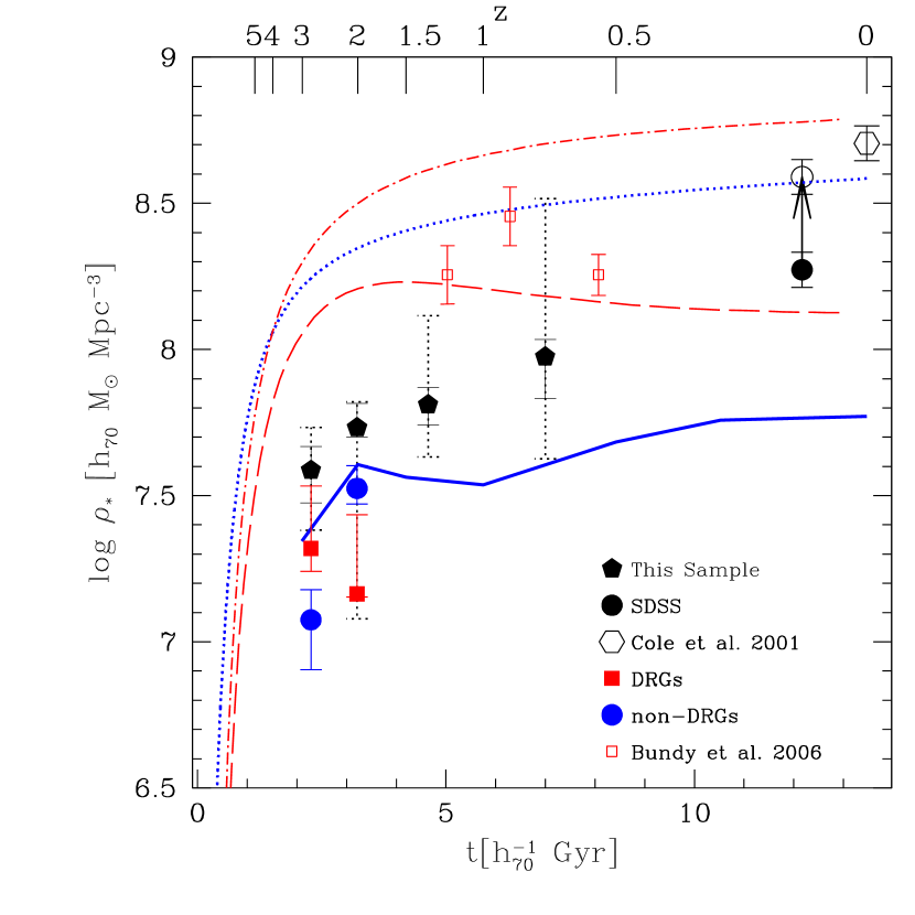
Figure 11.— A comparison of the evolution of of $\rho_{\star}$ with the predictions of theoretical simulations. The solid pentagons are our $\rho_{\star}$ measurements for galaxies with ${\rm L}_{V}^{rest}$$>$${\rm L}_{V}^{\rm thresh}$, where the dotted errorbars indicate the minimum and maximum $\rho_{\star}$ values among our fields as an indication of the field-to-field variance. The solid circle is our measurement of $\rho_{\star}$ from SDSS for galaxies above the luminosity limit. The open circle is our estimate of the total $\rho_{\star}$ from SDSS and the arrow connecting them indicates our correction to total $\rho_{\star}$ for the low redshift point. The open hexagon is the total $\rho_{\star}$ measurement from Cole et al. (2001). The red empty squares indicate the $\rho_{\star}$ values from Bundy et al. (2006) derived for all galaxies with ${\rm L}_{V}^{rest}$$>$${\rm L}_{V}^{\rm thresh}$. The dotted blue curve is the integral of the analytical SFR($z$) curve from Springel & Hernquist (2003), which represents the total $\rho_{\star}$ from that simulation. The solid blue curve is from a mock catalog created from the SH03 simulation (Finlator et al., 2006) and is for simulated galaxies with ${\rm L}_{V}^{rest}$$>$${\rm L}_{V}^{\rm thresh}$. The results of the Millennium simulation (Springel et al., 2005; Croton et al., 2005) are plotted as red curves. The dot-dashed red curve corresponds to the total stellar mass density in the simulation and the dashed red curve corresponds to the mass density in simulated galaxies with ${\rm L}_{V}^{rest}$$>$${\rm L}_{V}^{\rm thresh}$. The total $\rho_{\star}$ for all simulations agree with the observations at $z\sim 0$. When compared to the data using the same observational cut the Finlator et al. (2006) simulations fail to match the ensemble of data at $z\lesssim 1.4$. The Millennium simulations, however, fail to match the observational data at $z\gtrsim 1.4$. We also show the $\rho_{\star}$ values for the non-DRGs and DRGs as filled blue circles and red squares respectively, in the two redshift bins where DRGs are selected.

5.4. Room for Improvement

There are various ways in which these measurements of $\rho_{\star}$ could be improved, each relating to specific sources of possible error:

$\bullet$ Field-to-field variations are still a major source of uncertainty and can best be addressed by the inclusion of many more fields with deep optical and NIR imaging data, preferably to $K\sim 23$.

$\bullet$ We are still limited in that we are using a rest-frame luminosity selected sample. With the deep IRAC data that are now becoming available more reliable and well constrained mass determinations may be possible for individual galaxies. Selection by rest-frame $K_{s}$-band will not entirely solve this problem. In addition to the model uncertainties pointed out in §4.5, Labbé et al. (2005) and Shapley et al. (2005) have demonstrated that there are still large (a factor of 6-13) variations in ${\cal M_{\star}}/{\rm L}_{K}$ for high redshift galaxies and van der Wel et al. (2006) have shown that ${\cal M_{\star}}/{\rm L}_{K}$ of early type galaxies evolves by a factor of $\sim 3$ over $0<z<1$. An IRAC-selected sample will not be the same as a stellar mass-selected sample.

$\bullet$ There are few tests of photometric redshifts for galaxies with very red optical-UV colors. Since it is impossible to measure spectroscopic redshifts for every object it is crucial to test photometric redshifts with extensive NIR spectroscopy performed with the new generation of multi-object NIR spectrographs. In addition, these observations can give us independent measures of the dynamical masses of galaxies and will provide additional constraints on the $\cal{M_{\star}}$ estimates.

$\bullet$ The uncertainty at the faint end of the luminosity/mass function is great. Very deep NIR and MIR observations will be needed to see if the evolution inferred from the rest-frame optically bright population can be extended to the population as a whole.

$\bullet$ Local studies are still inconclusive as to the existence of a universal IMF in the local Universe. It is not clear at this time how to directly constrain the intermediate mass IMF at high redshifts. Dynamical mass estimates or gravitational lensing measurements of galaxies in regions where the baryons are thought to dominate the total mass may provide some assistance.

6. Summary and Conclusions

In this paper we have presented the evolution in the properties of the volume averaged stellar population from $z=0$ to $z=3$. We have used deep NIR and optical imaging over $\sim 100$ square arcminutes in four disjoint fields to mitigate field-to-field variations. The deep NIR data allow us to select and analyze galaxies at rest-frame optical wavelengths, where dust extinction and stellar mass-to-light ratio variations are far less than in the rest-frame UV. We derived photometric redshifts for all objects lacking a spectroscopic redshift and measure rest-frame UV through optical luminosities of all galaxies at $z<3.2$. We create a rest-frame $V$-band luminosity selected sample with ${\rm L}_{V}^{rest}$$>3\times 10^{10}$${\rm~{}h_{70}^{-2}~{}L_{\odot}}$ above which we are complete at all redshifts.

From these individual measurements we construct volume averaged properties such as the luminosity density, $j^{\rm rest}_{\lambda}$, and color, e.g. $(U-B)_{rest}$ and $(B-V)_{rest}$. The redshift evolution in luminosity density and mean color is very different. As found in R03 for a much smaller sample, $j^{\rm rest}_{\rm V}$ is roughly constant within a factor of $\approx 2.2$ from $z\sim 3$ to $z=0$. This modest evolution is broadly consistent with the results of D03 and Giallongo et al. (2005). The evolution in the rest-frame colors, however, is dramatic and the colors become systematically redder with decreasing redshift. The colors of our SDSS comparison sample at $z=0.1$ are $(B-V)_{rest}$$=0.72$ and $(U-B)_{rest}$$=0.07$. In contrast the average color of luminous galaxies at $z\sim 3$ is $(B-V)_{rest}$$=0.40$ and $(U-B)_{rest}$$=-0.38$.

By averaging over the population as a whole we are also averaging over the individual SFHs of the galaxies and the resultant volume averaged SFH will be smoother than that of the individual galaxies. We expect the mean colors to be more easily modeled than those of individual galaxies, which presumably have bursty SFHs. We find that the mean colors at all redshifts lie close to the locus of morphologically normal local galaxies in $(B-V)_{rest}$ vs. $(U-B)_{rest}$ space but compared to the local sample are slightly bluer in $(U-B)_{rest}$ at a fixed $(B-V)_{rest}$. Some of this difference could result from photometric redshift errors but could also be indicative of a residual signature of bursts in the mean colors.

We derive the luminosity weighted volume averaged UV-optical rest-frame SED for all galaxies with ${\rm L}_{V}^{rest}$$>3\times 10^{10}$${\rm~{}h_{70}^{-2}~{}L_{\odot}}$. At all wavelengths the mean SED becomes gradually more red with decreasing redshift and at all redshifts is within the range of SEDs spanned by normal galaxies in the local Universe. Even at our highest redshift bin the volume average SED does not look like that of a starburst from Kinney et al. (1996) with little extinction but rather, is redder than an irregular template. We also compute the mean SED from DRGs chosen to have $(J_{s}-K_{s})$$>2.3$. This mean DRG SED redder than average in the rest-frame optical and in the rest-frame UV.

With simple models we transform the mean SED into an evolution in the global ${\cal M_{\star}}/{\rm L}_{V}$. Because the volume averaged SFH should be smoother than that of the individual galaxies it is therefore more appropriate to use smooth models to fit the mean SED than to fit the SEDs of individual galaxies. Nonetheless, the colors cannot be fit well at all redshifts with a single model having an exponential SFH and a constant dust obscuration and metallicity. We can, however, fit the average SED at each redshift reasonably well with some combination of the parameters, as long as they can change as a function of redshift. We use these model fits to derive luminosity weighted stellar mass-to-light ratios for all galaxies with ${\rm L}_{V}^{rest}$$>3\times 10^{10}$${\rm~{}h_{70}^{-2}~{}L_{\odot}}$. ${\cal M_{\star}}/{\rm L}_{V}$ also declines smoothly from $z=0.1$ to $z\sim 3$ with ${\cal M_{\star}}/{\rm L}_{V}$$=4.9$ and $0.5$ at $z=0.1$ and $z\sim 3$ respectively. There are strong variations in ${\cal M_{\star}}/{\rm L}_{V}$ across the population. The DRGs have an ${\cal M_{\star}}/{\rm L}_{V}$ a factor of $\approx 1.1$ and 3.6 higher than the non-DRGs in the $z=2.01$ and $z=2.8$ redshift bins. This is consistent with the results of Labbé et al. (2005) and Förster Schreiber et al. (2004) who modeled the SEDs of individual DRGs.

Multiplying the $j^{\rm rest}_{\rm V}$ and mean ${\cal M_{\star}}/{\rm L}_{V}$ measurements we derive the evolution in $\rho_{\star}$ out to $z\sim 3$. $\rho_{\star}$ in luminous galaxies declines by a factor of $4.8$ out to $z=3$. At $z\sim 2$ and 2.8, the DRGs contribute 30% and 64% of $\rho_{\star}$, showing that UV selection techniques miss much of the stellar mass at $1.6<z<3$ in rest-frame optically luminous galaxies.

We also compare our $\rho_{\star}$ measurements to a set of recent model predictions subjected to our same rest-frame luminosity cut and find a large disagreement between the models themselves and between the models and observations. The different models can match the observed evolution in $\rho_{\star}$ over a limited redshift range, but both models predict an evolution that is too shallow to match the observations. This therefore implies that the masses of luminous galaxies in the models, or their abundance, are not consistent with the observations.

To better understand how different types of galaxies contribute to the stellar mass budget at high redshifts it will be necessary to reduce our reliance on photometric redshifts by performing NIR spectroscopy on a representative sample of DRGs. This will confirm the redshifts of the optically faint population that contributes over 50% of the stellar mass at high redshift. Re-performing this experiment with IRAC data will reduce the uncertainty due to dust obscuration and obtaining very deep NIR/MIR imaging will allow us to constrain the low mass end of the galaxy stellar mass function.

Table 1Ultra-violet Rest-frame Luminosity Densities

$z$	${\rm Field(s)}$	$N_{tot}$	$N_{use}$	$j_{2200}$	$dj_{2200}$	$j_{2700}$	$dj_{2700}$
$(1)$	$(2)$	$(3)$	$(4)$	$(5)$	$(6)$	$(7)$	$(8)$
$0.73$	ALL	116	112	$-11.84$	$0.34$	$-12.61$	$0.14$
$1.33$	ALL	154	127	$-12.35$	$0.18$	$-12.68$	$0.14$
$2.01$	ALL	164	126	$-11.95$	$0.14$	$-12.38$	$0.13$
$2.80$	ALL	95	82	$-13.67$	$0.15$	$-13.84$	$0.14$
$0.73$	HDF-N	11	11	$-12.06$	$0.42$	$-12.79$	$0.41$
$1.33$	HDF-N	9	9	$-13.15$	$0.55$	$-13.46$	$0.50$
$2.01$	HDF-N	13	11	$-12.91$	$0.38$	$-13.18$	$0.37$
$2.80$	HDF-N	16	16	$-13.82$	$0.30$	$-14.02$	$0.30$
$0.73$	HDF-S	4	4	$-11.55$	$0.58$	$-12.12$	$0.60$
$1.33$	HDF-S	13	11	$-12.78$	$0.33$	$-13.22$	$0.33$
$2.01$	HDF-S	7	6	$-12.55$	$0.51$	$-12.84$	$0.50$
$2.80$	HDF-S	25	24	$-14.60$	$0.25$	$-14.73$	$0.24$
$1.33$	MS1054-03	36	34	$-12.64$	$0.24$	$-12.90$	$0.22$
$2.01$	MS1054-03	50	46	$-12.35$	$0.25$	$-12.77$	$0.24$
$2.80$	MS1054-03	54	42	$-13.27$	$0.22$	$-13.46$	$0.20$
$0.73$	CDF-S	101	97			$-12.62$	$0.15$
$1.33$	CDF-S	96	73	$-12.07$	$0.29$	$-12.44$	$0.22$
$2.01$	CDF-S	94	63	$-11.54$	$0.20$	$-12.04$	$0.18$

Note. — All luminosity densities are given in $h_{70}$ AB magnitudes $/$ Mpc³. (3) is the total number of galaxies in each bin with ${\rm L}_{V}^{rest}$$>$${\rm L}_{V}^{\rm thresh}$. In (4) we give the number of galaxies above our luminosity threshold that also have $\delta z/(1+z)\leq 0.16$. As described in §3.2 and R03 we calculate the $j^{\rm rest}_{\lambda}$values using the galaxies in (4), and correct for those galaxies that have been excluded due to their large photometric redshift uncertainties. The $z=0.73$ entry for MS1054-03 has been omitted because of the presence of a rich $z=0.83$ cluster in that field. The $z=2.80$ entry for the CDF-S has been omitted because of a high incompleteness at these redshifts caused by the moderate depth. The empty entry in columns (5) and (6) for the CDF-S is because $\lambda_{rest}=2200{\rm\AA}$ was blueward of the bluest observed filter.

Table 2Optical Rest-frame Luminosity Densities

$z$	${\rm Field(s)}$	$j_{U}$	$dj_{U}$	$j_{B}$	$dj_{B}$	$j_{V}$	$dj_{V}$
$(1)$	$(2)$	$(3)$	$(4)$	$(5)$	$(6)$	$(7)$	$(8)$
$0.73$	ALL	$-13.86$	$0.12$	$-14.82$	$0.12$	$-15.40$	$0.12$
$1.33$	ALL	$-13.73$	$0.09$	$-14.52$	$0.09$	$-14.98$	$0.09$
$2.01$	ALL	$-13.53$	$0.09$	$-14.31$	$0.09$	$-14.78$	$0.08$
$2.80$	ALL	$-14.55$	$0.11$	$-15.05$	$0.12$	$-15.35$	$0.12$
$0.73$	HDF-N	$-14.12$	$0.40$	$-15.15$	$0.38$	$-15.73$	$0.37$
$1.33$	HDF-N	$-14.26$	$0.41$	$-15.03$	$0.39$	$-15.52$	$0.41$
$2.01$	HDF-N	$-14.01$	$0.28$	$-14.59$	$0.28$	$-14.93$	$0.30$
$2.80$	HDF-N	$-14.48$	$0.31$	$-14.90$	$0.29$	$-15.20$	$0.28$
$0.73$	HDF-S	$-13.21$	$0.59$	$-14.12$	$0.61$	$-14.64$	$0.62$
$1.33$	HDF-S	$-14.36$	$0.26$	$-15.17$	$0.27$	$-15.62$	$0.26$
$2.01$	HDF-S	$-13.63$	$0.40$	$-14.20$	$0.38$	$-14.46$	$0.38$
$2.80$	HDF-S	$-15.22$	$0.21$	$-15.70$	$0.19$	$-15.93$	$0.19$
$1.33$	MS1054-03	$-13.72$	$0.18$	$-14.43$	$0.17$	$-14.85$	$0.17$
$2.01$	MS1054-03	$-13.76$	$0.18$	$-14.55$	$0.17$	$-15.00$	$0.17$
$2.80$	MS1054-03	$-14.35$	$0.15$	$-14.89$	$0.16$	$-15.21$	$0.17$
$0.73$	CDF-S	$-13.87$	$0.13$	$-14.83$	$0.13$	$-15.40$	$0.12$
$1.33$	CDF-S	$-13.62$	$0.12$	$-14.44$	$0.11$	$-14.91$	$0.11$
$2.01$	CDF-S	$-13.37$	$0.11$	$-14.18$	$0.11$	$-14.69$	$0.11$

Note. — All luminosity densities are given in $h_{70}$ AB magnitudes $/$ Mpc³ with the following conversion to Vega magnitudes: $U_{vega}=U_{AB}-0.79$, $B_{vega}=B_{AB}+0.102$, $V_{vega}=V_{AB}-0.008$. The $z=0.73$ entry for MS1054-03 has been omitted because of the presence of a rich $z=0.83$ cluster in that field. The $z=2.80$ entry for the CDF-S has been omitted because of a high incompleteness at these redshifts caused by the moderate depth.

Table 3Stellar Mass Densities

$z$	${\rm L}_{V}^{\rm thresh}$	${\rm log}(\rho_{\star})$	${\rm log}(\rho_{\star,low})$	${\rm log}(\rho_{\star,high})$	${\rm log}(\rho_{\star,low,f2f})$	${\rm log}(\rho_{\star,high,f2f})$
$(1)$	$(2)$	$(3)$	$(4)$	$(5)$	$(6)$	$(7)$
$0.1$	0	$8.59$	$8.55$	$8.63$
$0.1$	$3\times 10^{10}$	$8.27$	$8.23$	$8.31$
$0.73$	$3\times 10^{10}$	$7.97$	$7.83$	$8.03$	$7.63$	$8.52$
$1.33$	$3\times 10^{10}$	$7.81$	$7.74$	$7.87$	$7.63$	$8.12$
$2.01$	$3\times 10^{10}$	$7.73$	$7.70$	$7.82$	$7.08$	$7.82$
$2.80$	$3\times 10^{10}$	$7.59$	$7.47$	$7.67$	$7.38$	$7.73$
$0.1$	$0.3\times 10^{10}$	$8.59$	$8.55$	$8.63$
$0.73$	$1.3\times 10^{10}$	$8.05$	$8.02$	$8.12$	$7.86$	$8.52$
$1.33$	$1.3\times 10^{10}$	$7.87$	$7.83$	$7.94$	$7.74$	$8.22$
$2.01$	$1.3\times 10^{10}$	$7.76$	$7.70$	$7.82$	$7.31$	$7.89$
$2.80$	$3\times 10^{10}$	$7.59$	$7.48$	$7.65$	$7.38$	$7.73$

Note. — (2) is given in units of ${\rm h_{70}^{-2}~{}L_{V,\odot}}$. (3)–(7) are given in units of ${\rm h_{70}}~{}{\cal M_{\odot}}$ Mpc^-3 and are for all galaxies with ${\rm L}_{V}^{rest}$$>$${\rm L}_{V}^{\rm thresh}$. The first 2 rows indicate our measurements for the SDSS. (4) and (5) are the formal confidence limits on $\rho_{\star}$. (6) and (7) give the range in $\rho_{\star}$ allowed by the rms field-to-field variations among our different fields.

Table 4Mean Mass-to-light ratios

$z$	${\rm Field(s)}$	$\langle M_{\star}/L_{V}\rangle$	$\langle{\cal M_{\star}}/L_{V}\rangle_{low}$	$\langle M_{\star}/L_{V}\rangle_{high}$
$(1)$	$(2)$	$(3)$	$(4)$	$(5)$
$0.73$	ALL	$1.06$	$0.77$	$1.18$
$1.33$	ALL	$1.07$	$0.88$	$1.18$
$2.01$	ALL	$1.08$	$0.97$	$1.19$
$2.80$	ALL	$0.46$	$0.39$	$0.50$
$0.73$	HDF-N	$1.30$	$1.06$	$1.44$
$1.33$	HDF-N	$0.97$	$0.65$	$1.18$
$2.01$	HDF-N	$0.58$	$0.40$	$0.76$
$2.80$	HDF-N	$0.33$	$0.15$	$0.39$
$0.73$	HDF-S	$0.96$	$0.85$	$1.36$
$1.33$	HDF-S	$1.19$	$0.78$	$1.26$
$2.01$	HDF-S	$0.32$	$0.28$	$0.62$
$2.80$	HDF-S	$0.37$	$0.22$	$0.43$
$1.33$	MS1054-03	$0.80$	$0.71$	$0.97$
$2.01$	MS1054-03	$1.08$	$0.78$	$1.19$
$2.80$	MS1054-03	$0.50$	$0.37$	$0.62$
$0.73$	CDF-S	$1.06$	$0.96$	$1.06$
$1.33$	CDF-S	$1.08$	$0.78$	$1.18$
$2.01$	CDF-S	$1.26$	$1.03$	$1.39$

Note. — Columns (3)-(5) are computed for all galaxies with ${\rm L}_{V}^{rest}$$>$${\rm L}_{V}^{\rm thresh}$ and are in units of $[{\cal M_{\odot}}/L_{\odot}]$. The $z=0.73$ entry for MS1054-03 has been omitted because of the presence of a rich $z=0.83$ cluster in that field. The $z=2.80$ entry for the CDF-S has been omitted because of a high incompleteness at these redshifts caused by the moderate depth.

Table 5Relative Stellar Mass Densities

$z$	${\rm Field(s)}$	$\Delta\rho_{\star}$	$\Delta\rho_{\star,low}$	$\Delta\rho_{\star,high}$	$\Delta\rho_{\star,low}^{corr}$	$\Delta\rho_{\star,high}^{corr}$
$(1)$	$(2)$	$(3)$	$(4)$	$(5)$	$(6)$	$(7)$
$0.73$	ALL	$0.39$	$0.28$	$0.44$	$0.21$	$0.44$
$1.33$	ALL	$0.27$	$0.23$	$0.30$	$0.13$	$0.30$
$2.01$	ALL	$0.22$	$0.21$	$0.27$	$0.10$	$0.27$
$2.80$	ALL	$0.16$	$0.12$	$0.19$	$0.06$	$0.19$
$0.73$	HDF-N	$0.64$	$0.38$	$0.83$	$0.18$	$0.83$
$1.33$	HDF-N	$0.39$	$0.19$	$0.57$	$0.09$	$0.57$
$2.01$	HDF-N	$0.14$	$0.08$	$0.22$	$0.04$	$0.22$
$2.80$	HDF-N	$0.10$	$0.05$	$0.13$	$0.02$	$0.13$
$0.73$	HDF-S	$0.17$	$0.07$	$0.32$	$0.04$	$0.32$
$1.33$	HDF-S	$0.53$	$0.33$	$0.69$	$0.16$	$0.69$
$2.01$	HDF-S	$0.05$	$0.04$	$0.10$	$0.02$	$0.10$
$2.80$	HDF-S	$0.22$	$0.13$	$0.28$	$0.06$	$0.28$
$1.33$	MS1054-03	$0.18$	$0.14$	$0.22$	$0.07$	$0.22$
$2.01$	MS1054-03	$0.27$	$0.19$	$0.33$	$0.09$	$0.33$
$2.80$	MS1054-03	$0.15$	$0.10$	$0.21$	$0.05$	$0.21$
$0.73$	CDF-S	$0.39$	$0.34$	$0.44$	$0.16$	$0.44$
$1.33$	CDF-S	$0.25$	$0.19$	$0.29$	$0.09$	$0.29$
$2.01$	CDF-S	$0.24$	$0.20$	$0.29$	$0.10$	$0.29$

Note. — The relative mass densities in (3) are given in terms of the fractional decrease from $z=0$, i.e. $\Delta\rho_{\star}=\rho_{\star}/\rho_{\star}(z=0)$, as computed by correcting the values to total using the SDSS data and using the $z=0$ measurement of Cole et al. (2001). The confidence intervals in $\Delta\rho_{\star}$ given in columns (4) and (5) come from the formal uncertainties on this evolution for galaxies with ${\rm L}_{V}^{rest}$$>$${\rm L}_{V}^{\rm thresh}$. The confidence intervals in columns (6) and (7) include the extra uncertainty that comes from allowing ${\rm L}_{V}^{\rm thresh}$ to evolve with redshift according to the evolution in ${\cal M_{\star}}/{\rm L}_{V}$. The $z=0.73$ entry for MS1054-03 has been omitted because of the presence of a rich $z=0.83$ cluster in that field. The $z=2.80$ entry for the CDF-S has been omitted because of a high incompleteness at these redshifts caused by the moderate depth.

Appendix A The Effect of Weak Lensing on the Luminosity Density

Weak lensing of background galaxies by a foreground mass distribution affects the luminosity density of the background sources by changing their apparent magnitudes, surface densities, and the volume enclosed in the observed solid angle. To the first order all of these effects are directly dependent on the magnification factor $\mu$. Given a mass map for the foreground cluster and the redshift of each source it is possible to compute the magnifications of each source $\mu_{i}$.

First we consider the effect of weak lensing on the total integrated luminosity density in a given redshift slice whose enclosed co-moving volume per unit solid angle is $V_{0}$, in units of $[{\rm Mpc^{3}/ster}]$. The “true” luminosity density, i.e. in the absence of lensing, is $j_{o}$. This can be written as:

$$j_{0}=\frac{n_{0}}{V_{0}}\sum_{i=0}^{n_{gal}}\frac{L_{0,i}}{n_{gal}}~{}\left[\frac{\rm L_{\odot}}{\rm Mpc^{3}}\right],$$ (A1)

where $n_{0}$ is the surface density of sources in units of $[{\rm ster}^{-1}]$. $n_{0}$ can be written as

$$n_{0}=N_{0}V_{0}~{}[{\rm ster}^{-1}],$$ (A2)

where $N_{0}$ is the intrinsic volume number density in units of $[{\rm\#/Mpc^{3}}]$. We can now rewrite $j_{0}$ as

$$j_{0}=N_{0}\sum_{i=0}^{n_{gal}}\frac{L_{0,i}}{n_{gal}}~{}\left[{\rm L_{\odot}/Mpc^{3}}\right].$$ (A3)

Under the influence of lensing the rest-frame luminosities (which is what we derive from observed magnitudes) become

$$L_{\ell,i}=L_{0,i}\mu_{i}$$ (A4)

while the intrinsic volume number density naturally remains unaffected. The luminosity density subject to lensing $j_{\ell}$ is therefore

$$j_{\ell}=N_{0}\sum_{i=0}^{n_{gal}}\frac{L_{0,i}\mu_{i}}{n_{gal}}=\frac{n_{0}}{V_{0}}\sum_{i=0}^{n_{gal}}\frac{L_{0,i}\mu_{i}}{n_{gal}}~{}\left[{\rm L_{\odot}/Mpc^{3}}\right].$$ (A5)

Since the sole difference between $j_{\ell}$ and $j_{0}$ is the magnification of the individual sources, we compute $j_{0}$ in MS1054-03 by using the demagnified galaxy luminosities, $L_{0,i}=L_{\ell,i}/\mu_{i}$. The $\mu_{i}$ are determined from the weak lensing map of Hoekstra et al. (2000).

The second effect stems from the use of a fixed luminosity limit in the presence of magnification. For example, sources whose intrinsic luminosities would exclude them from the sample can enter the sample after being magnified. At all but the highest redshifts in the MS1054-03 field our data are complete significantly below the luminosity limit. Therefore to correct for this effect in our analysis we select galaxies brighter than ${\rm L}_{V}^{\rm thresh}$ based on their demagnified luminosities.

References

- Adelberger et al. (2004) Adelberger, K. L., Steidel, C. C., Shapley, A. E., Hunt, M. P., Erb, D. K., Reddy, N. A., & Pettini, M. 2004, ApJ, 607, 226
- Baldry et al. (2002) Baldry, I. K. et al. 2002, ApJ, 569, 582
- Baugh et al. (2005) Baugh, C. M., Lacey, C. G., Frenk, C. S., Granato, G. L., Silva, L., Bressan, A., Benson, A. J., & Cole, S. 2005, MNRAS, 356, 1191
- Bell et al. (2003) Bell, E. F., McIntosh, D. H., Katz, N., & Weinberg, M. D. 2003, ApJ, 585, L117
- Bell et al. (2004) Bell, E. F., et al. 2004, ApJ, 608, 752
- Bershady et al. (1998) Bershady, M. A., Lowenthal, J. D., & Koo, D. C. 1998, ArXiv Astrophysics e-prints, arXiv:astro-ph/9804093
- Bertin & Arnouts (1996) Bertin, E. & Arnouts, S. 1996, A&AS, 117, 393
- Bessell & Brett (1988) Bessell, M. S. & Brett, J. M. 1988, PASP, 100, 1134
- Bessell (1990) Bessell, M. S. 1990, PASP, 102, 1181
- Blanton et al. (2003a) Blanton, M. R. et al. 2003a, ApJ, 594, 186
- Blanton et al. (2003b) Blanton, M. R. et al. 2003b, ApJ, 592, 819
- Bolzonella et al. (2000) Bolzonella, M., Miralles, J.-M., & Pelló, R. 2000, A&A, 363, 476
- Borch et al. (2006) Borch, A. et al. 2006, A&Ain press, astro-ph/0604405
- Brinchmann & Ellis (2000) Brinchmann, J. & Ellis, R. S. 2000, ApJ, 536, L77
- Brinchmann et al. (2004) Brinchmann, J., Charlot, S., White, S. D. M., Tremonti, C., Kauffmann, G., Heckman, T., & Brinkmann, J. 2004, MNRAS, 351, 1151
- Bruzual & Charlot (2003) Bruzual, G., & Charlot, S. 2003, MNRAS, 344, 1000
- Bundy et al. (2006) Bundy, K., & et al. 2006, submitted to ApJ, astro-ph/0512465
- Calzetti et al. (2000) Calzetti, D., Armus, L., Bohlin, R. C., Kinney, A. L., Koornneef, J., & Storchi-Bergmann, T. 2000, ApJ, 533, 682
- Casertano et al. (2000) Casertano, S. et al. 2000, AJ, 120, 2747
- Chabrier (2003) Chabrier, G. 2003, PASP, 115, 763
- Cole et al. (2001) Cole, S. et al. 2001, MNRAS, 326, 255
- Coleman, Wu, & Weedman (1980) Coleman, G. D., Wu, C. -C., & Weedman, D. W. 1980, ApJS, 43, 393
- Croton et al. (2005) Croton, D. et al. 2005, submitted to MNRAS, astro-ph/0508046
- Daddi et al. (2003) Daddi, E. et al. 2003, ApJ, 588, 50
- Daddi et al. (2004) Daddi, E., Cimatti, A., Renzini, A., Fontana, A., Mignoli, M., Pozzetti, L., Tozzi, P., & Zamorani, G. 2004, ApJ, 617, 746
- Daddi et al. (2005) Daddi, E., et al. 2005, ApJ, 680, 697
- de Mello et al. (2004) de Mello, D. F., Daddi, E., Renzini, A., Cimatti, A., di Serego Alighieri, S., Pozzetti, L., & Zamorani, G. 2004, ApJ, 608, L29
- Dickinson (1999) Dickinson, M. 1999, AIP Conf. Proc. 470: After the Dark Ages: When Galaxies were Young (the Universe at ), 470, 122
- Dickinson et al. (2000) Dickinson, M., et al. 2000, ApJ, 531, 624
- Dickinson, Papovich, Ferguson, & Budavári (2003) Dickinson, M., Papovich, C., Ferguson, H. C., & Budavári, T. 2003, ApJ, 587, 25
- Drory et al. (2004) Drory, N., Bender, R., Feulner, G., Hopp, U., Maraston, C., Snigula, J., & Hill, G. J. 2004, ApJ, 608, 742
- Drory et al. (2005) Drory, N., Salvato, M., Gabasch, A., Bender, R., Hopp, U., Feulner, G., & Pannella, M. 2005, ApJ, 619, L131
- Ferguson & Johnson (2001) Ferguson, A. M. N., & Johnson, R. A. 2001, ApJ, 559, L13
- Finlator et al. (2006) Finlator, K., Davé, R., Papovich, C., Hernquist, L. 2006, ApJ, 639, 672
- Förster Schreiber et al. (2004) Förster Schreiber, N. M., et al. 2004, ApJ, 616, 40
- Förster Schreiber et al. (2006) Förster Schreiber, N. M., et al. 2006, AJin press, astro-ph/0510186
- Fontana et al. (2003) Fontana, A. et al. 2003, ApJ, 594, L9
- Fontana et al. (2004) Fontana, A., et al. 2004, A&A, 424, 23
- Franx et al. (2003) Franx, M. et al. 2003, ApJ, 587, L79
- Gabasch et al. (2004) Gabasch, A., et al. 2004, A&A, 421, 41
- Giallongo et al. (2005) Giallongo, E., Salimbeni, S., Menci, N., Zamorani, G., Fontana, A., Dickinson, M., Cristiani, S., & Pozzetti, L. 2005, ApJ, 622, 116
- Giavalisco & Dickinson (2001) Giavalisco, M. & Dickinson, M. 2001, ApJ, 550, 177
- Gilli et al. (2003) Gilli, R., et al. 2003, ApJ, 592, 721
- Glazebrook et al. (2003) Glazebrook, K. et al. 2003, ApJ, 587, 55
- Glazebrook et al. (2004) Glazebrook, K., et al. 2004, Nature, 430, 181
- Hammer et al. (2005) Hammer, F., Flores, H., Elbaz, D., Zheng, X. Z., Liang, Y. C., & Cesarsky, C. 2005, A&A, 430, 115
- Hansen et al. (2002) Hansen, B. M. S., et al. 2002, ApJ, 574, L155
- Hauschildt, Allard, & Baron (1999) Hauschildt, P. H., Allard, F., & Baron, E. 1999, ApJ, 512, 377
- Hoekstra et al. (2000) Hoekstra, H., Franx, M., & Kuijken, K. 2000, ApJ, 532, 88
- Hogg et al. (1997) Hogg, D. W., Neugebauer, G., Armus, L., Matthews, K., Pahre, M. A., Soier, B. T., & Weinberger, A. J. 1997, AJ, 113, 474
- Hogg et al. (2002) Hogg, D. W. et al. 2002, AJ, 124, 646
- Jansen et al. (2000a) Jansen, R. A., Franx, M., Fabricant, D., & Caldwell, N. 2000, ApJS, 126, 271
- Jansen et al. (2000b) Jansen, R. A., Fabricant, D., Franx, M., & Caldwell, N. 2000, ApJS, 126, 331
- Kauffmann et al. (2003) Kauffmann, G. et al. 2003, MNRAS, 341, 33
- Kennicutt et al. (1994) Kennicutt, R. C., Tamblyn, P., & Congdon, C. E. 1994, ApJ, 435, 22
- Kinney et al. (1996) Kinney, A. L., Calzetti, D., Bohlin, R. C., McQuade, K., Storchi-Bergmann, T., & Schmitt, H. R. 1996, ApJ, 467, 38
- Kriek et al. (2006) Kriek, M., submitted to ApJ
- Labbé et al. (2003) Labbé, I. et al. 2003, AJ, 125, 1107
- Labbé et al. (2005) Labbé, I., et al. 2005, ApJ, 624, L81
- Larson & Tinsley (1978) Larson, R. B. & Tinsley, B. M. 1978, ApJ, 219, 46
- Le Floc’h et al. (2005) Le Floc’h, E., et al. 2005, ApJ, 632, 169
- Madau, Pozzetti, & Dickinson (1998) Madau, P., Pozzetti, L., & Dickinson, M. 1998, ApJ, 498, 106
- Maraston (2005) Maraston, C. 2005, MNRAS, 362, 799
- Marchesini et al. (2006) Marchesini, D. in prep
- Matteucci (1994) Matteucci, F. 1994, A&A, 288, 57
- Moorwood (1997) Moorwood, A. F. 1997, Proc. SPIE, 2871, 1146
- Nagamine et al. (2004) Nagamine, K., Cen, R., Hernquist, L., Ostriker, J. P., & Springel, V. 2004, ApJ, 610, 45
- Nagashima et al. (2005) Nagashima, M., Lacey, C. G., Okamoto, T., Baugh, C. M., Frenk, C. S., & Cole, S. 2005, MNRAS, 363, L31
- Papovich, Dickinson, & Ferguson (2001) Papovich, C., Dickinson, M., Ferguson, H. C., 2001, ApJ, 559, 620
- Papovich et al. (2005) Papovich, C., Dickinson, M., Giavalisco, M., Conselice, C. J., & Ferguson, H. C. 2005, ApJ, in press, astro-ph/0501088
- Pei, Fall, & Hauser (1999) Pei, Y. C., Fall, S. M., & Hauser, M. G. 1999, ApJ, 522, 604
- Pettini et al. (2000) Pettini, M., Steidel, C. C., Adelberger, K. L., Dickinson, M., & Giavalisco, M. 2000, ApJ, 528, 96
- Prévot et al. (1984) Prévot, M. L., Lequeux, J., Prevot, L., Maurice, E., & Rocca-Volmerange, B. 1984, A&A, 132, 389
- Reddy et al. (2005) Reddy, N., Erb, D., Steidel, C., Shapley, A, Adelberger, K., Pettini, M., 2005, ApJ, in press, astro-ph/0507264
- Rudnick et al. (2001) Rudnick, G., Franx, M., Rix, H.-W., Moorwood, A., Kuijken, K., van Starkenburg, L., van der Werf, P., Röttgering, H., Labbé, I. 2001, AJ, 122, 2205
- Rudnick et al. (2003) Rudnick, G., et al. 2003, ApJ, 599, 847
- Salpeter (1955) Salpeter, E. E. 1955, ApJ, 121, 161
- Sawicki, Lin, & Yee (1997) Sawicki, M. J., Lin, H., & Yee, H. K. C. 1997, AJ, 113, 1
- Shapley et al. (2001) Shapley, A. E., Steidel, C. C., Adelberger, K. L., Dickinson, M., Giavalisco, M., & Pettini, M. 2001, ApJ, 562, 95
- Shapley et al. (2004) Shapley, A. E., Erb, D. K., Pettini, M., Steidel, C. C., & Adelberger, K. L. 2004, ApJ, 612, 108
- Shapley et al. (2005) Shapley, A. E., Steidel, C. C., Erb, D. K., Reddy, N. A., Adelberger, K. L., Pettini, M., Barmby, P., & Huang, J. 2005, ApJ, 626, 698
- Smail et al. (1997) Smail, I., Ivison, R. J., & Blain, A. W. 1997, ApJ, 490, L5
- Somerville et al. (2004) Somerville, R. S., Lee, K., Ferguson, H. C., Gardner, J. P., Moustakas, L. A., & Giavalisco, M. 2004, ApJ, 600, L171
- Springel & Hernquist (2003) Springel, V., & Hernquist, L. 2003, MNRAS, 339, 312
- Springel et al. (2005) Springel, V. et al. 2005, Nature, 435, 629
- Steidel et al. (1996) Steidel, C. C., Giavalisco, M., Pettini, M., Dickinson, M., & Adelberger, K. L. 1996, ApJ, 462, L17
- Steidel et al. (1999) Steidel, C. C., Adqelberger, K. L., Giavalisco, M., Dickinson, M., & Pettini, M. 1999, ApJ, 519, 1
- Steidel et al. (2004) Steidel, C. C., Shapley, A. E., Pettini, M., Adelberger, K. L., Erb, D. K., Reddy, N. A., & Hunt, M. P. 2004, ApJ, 604, 534
- Stoughton et al. (2002) Stoughton, C. et al. 2002, AJ, 123, 485
- Strauss et al. (2002) Strauss, M. A. et al. 2002, AJ, 124, 1810
- Thomas et al. (2005) Thomas, D., Maraston, C., Bender, R., & de Oliveira, C. M. 2005, ApJ, 621, 673
- Trager et al. (2000) Trager, S. C., Faber, S. M., Worthey, G., & González, J. J. 2000, AJ, 119, 1645
- van der Wel et al. (2004) van der Wel, A., Franx, M., van Dokkum, P. G., & Rix, H.-W. 2004, ApJ, 601, L5
- van der Wel et al. (2006) van der Wel, A., Franx, M., van Dokkum, P. G., Huang, J., Rix, H.-W., & Illingworth, G. D. 2006, ApJ, 636, L21
- van Dokkum & Franx (1996) van Dokkum, P. G., & Franx, M. 1996, MNRAS, 281, 985
- van Dokkum et al. (2000) van Dokkum, P.G., Franx, M., Fabricant, D., Illingworth, G.D., & Kelson, D.D. 2000, ApJ, 541, 95
- van Dokkum et al. (2003) van Dokkum, P. G. et al. 2003, ApJ, 587, L83
- van Dokkum et al. (2004) van Dokkum, P. G., et al. 2004, ApJ, 611, 703
- van Dokkum et al. (2006) van Dokkum, P. G., et al. 2005, submitted to ApJ
- Williams et al. (1996) Williams, R. E. et al. 1996, AJ, 112, 1335
- Wolf et al. (2003) Wolf, C., Meisenheimer, K., Rix, H.-W., Borch, A., Dye, S., & Kleinheinrich, M. 2003, A&A, 401, 73
- Wuyts et al. (in preparation) Wuyts, S. et al. in preparation
- York et al. (2000) York, D. G. et al. 2000, AJ, 120, 1579