The slope of the GRB Variability/Peak Luminosity Correlation

Abstract

First using a sample of 32 GRBs with known redshift (Guidorzi et al. 2005) and then a sample of 551 BATSE GRBs with derived pseudo-redshift (Guidorzi 2005), the time variability/peak luminosity correlation ($V$ vs. $L$), originally found by Reichart et al. (2001) using a sample of 18 GRBs, was tested. For both samples the correlation is still found but less relevant due to a much higher spread of the data. Assuming a straight line in the $\log{L}$–$\log{V}$ plane ($\log{L}=m\log{V}+b$), as done by Reichart et al., both Guidorzi et al. and Guidorzi found that the line slope for both samples is much lower than that derived by Reichart et al.: $m=1.3_{-0.4}^{+0.8}$ (Guidorzi et al. 2005), $m=0.85\pm 0.02$ (Guidorzi 2005), $m=3.3^{+1.1}_{-0.9}$ (Reichart et al. 2001). Reichart & Nysewander (2005) discuss our results and attribute the different slope to the fact we do not take into account in the fit the variance of the sample (also called slop), and demonstrate that, using the method presented by Reichart (2001), the expanded data set of Guidorzi et al. (2005) in $\log{L}$–$\log{V}$ plane is still well described by a line with slope $m=3.4^{+0.9}_{-0.6}$. Here we compare the results of two methods accounting for the slop of the sample, the method implemented by Reichart (2001) and that by D’Agostini (2005). We demonstrate that the method used by Reichart et al. (2001) to estimate the straight line slope, provides an inconsistent estimate of the parameter when the sample variance is comparable with the interval of values covered by the GRB variability. We also demonstrate that, using the D’Agostini method, the slope of the $\log{L}$–$\log{V}$ correlation is still consistent with that derived by us earlier and inconsistent with that derived by Reichart & Nysewander (2005). Finally we discuss the implications on the interpretations proposed for the $V-L$ correlation and show that our results are in agreement with the peak energy/variability correlation found by Lloyd-Ronning & Ramirez-Ruiz (2002) and the peak energy/peak luminosity correlation (Yonetoku et al. 2004; Ghirlanda et al. 2005).

1 Introduction

Most of our knowledge about the Gamma-Ray Burst (GRB) phenomenon is derived from their spectra and light curve profiles, but it is recognised that other observational probes (e.g., polarisation of the gamma-rays) would give key information to the solution of the GRB enigma. Among these probes, it is recognised the importance of the erratic time variability of the GRB time profiles. For example, in the GRB internal shock model, not very variable radiation is expected to be produced at radii lower than the photosphere radius in which the shocks remain optically thin to pairs (Kobayashi et al., 2002), while highly variable radiation is expected to be produced in shocks above this radius (Mészáros et al., 2002). Also in the sub-jet model by Ioka & Nakamura (2001), time variability is expected and its amplitude related to the viewing angle of the burst.

A key objective of the study of GRBs is to establish whether GRBs can be reliably used as standard candles and to determine the optimal relationship between observed and intrinsic properties. The recent discovery of GRBs with bright afterglows at redshifts $z>6$ highlights their power as probes of the high redshift Universe (Haislip et al., 2006; Kawai et al., 2006), but spectroscopically-confirmed redshifts are only a fraction. In contrast, the characteristics of gamma-ray light curves, which are available for all GRBs, offer a potentially independent estimate of luminosity distance for statistically-significant samples.

An important problem, however, in deriving the intrinsic correlations is the interpretation of scatter in correlations, which may be produced by measurement methods, construction of samples with properties measured by satellites with differing response functions, small samples and different statistical analysis methods and intrinsic physical differences in the GRB population (Nava et al., 2006). As sample sizes slowly increase, addressing these issues remains critical for the correct inference of intrinsic GRB properties and thus their use as cosmological probes.

In this paper, we concentrate on a long-standing empirical relation that initially suggested a possible Cepheid-like correlation between gamma-ray variability and peak luminosity of GRBs (Reichart et al., 2001; Fenimore & Ramirez-Ruiz, 2000).

Reichart et al. (2001) (hereafter R01), using a robust measure $V$ of the GRB variability, for a sample of 13 GRBs with known redshift, found that in the GRB rest frame this measure is correlated with the GRB peak luminosity $L$. In the $\log{L}$–$\log{V}$ plane the correlation was modelled with a linear function $\log L=m\log V+b$ with the slope of the straight line $m=3.3^{+1.1}_{-0.9}$ and a sample variance along $V$ of $\sigma_{\log{V}}=0.18$, both parameters being obtained with the method described by Reichart (2001) (hereafter called Reichart method). This method was proposed to fit data sets affected by a sample variance in addition to the statistical variance (called ”intrinsic variance”) of each data point. Recently, first Guidorzi et al. (2005) (hereafter GFM05) and then Guidorzi (2005) (hereafter G05) tested this correlation first using an extended sample of 32 GRBs with known redshift (GFM05), and then with 551 GRBs detected by CGRO/BATSE (Paciesas et al., 1999) for which a pseudo-redshift was derived by G05 exploiting the spectral lag-luminosity correlation (Norris et al., 2000; Norris, 2002; Band et al., 2004). In both cases, the correlation was confirmed and in the $\log V$–$\log L$ plane the slope of the straight line was found much lower than that derived by R01 ($m=1.3_{-0.4}^{+0.8}$ derived by GFM05; $m=0.85\pm 0.02$ derived by G05). It was also found that, with the sample variance neglected, the straight line did not provide a good description of the data ($\chi^{2}/{\rm dof}=1167/30$ and $\chi^{2}/{\rm dof}=4238/549$ for the samples considered by GFM05 and G05, respectively). Neglecting the sample variance was correctly questioned by Reichart & Nysewander (2005) (hereafter RN05), who however show that, also using the extended data set of GFM05, the $m$ slope is given by $m=3.4_{-0.6}^{+0.9}$, still in perfect agreement with the original value found by R01 and in strong disagreement with the value found by GFM05. They attribute this disagreement to the fact that GFM05 do not include among the parameters of the fit the sample variance, which they estimate to be $\sigma_{\log{V}}=0.20\pm 0.04$. In an unrefereed note, Reichart (2005) takes issue with the most recent paper by G05, who confirms the results previously found by GFM05.

In this paper, we discuss the Reichart method and compare the results with those obtained following the treatment by D’Agostini (2005) (hereafter called “the D’Agostini method”), which deals with the same problem of fitting data points affected by extrinsic scatter in addition the intrinsic uncertainties along both axes. We show with numerical simulations that the Reichart method provides an inconsistent estimate of the $m$ slope in the specific case of the $\log V$–$\log L$ data set, we discuss the likely reason for this inconsistency. We show that our original results are substantially confirmed by the D’Agostini method even taking into account the sample variance. Finally we discuss the subsequent implications for the inferred physics of GRB central engines and their relativistic outflows. The usefulness of the so-called variability/peak luminosity correlation is discussed in the broader context of recently discovered correlations between other observed and derived properties of GRBs.

2 The Reichart method

The Reichart method has as starting point the well known Bayes theorem that, for inference of physical parameters, is widely discussed in several text books (see, e.g., D’Agostini 2003). It states that the conditional probability that a set of parameters $\theta$$=\theta_{1},\theta_{2},...\theta_{n}$ takes a particular value $\mbox{\boldmath$\theta$}^{0}$, given a data set $D$, whose values depend on $\theta$ (for instance, N independent observations of a quantity $X$), is given by:

$$p(\mbox{\boldmath$\theta$}|DI)=\frac{p(\mbox{\boldmath$\theta$}|I)\ p(D|\mbox{\boldmath$\theta$}I)}{p(D|I)}$$ (1)

where $I$ is the available prior information, $p(\mbox{\boldmath$\theta$}|I)$ is the probability distribution of $\theta$ on the basis of the information $I$, and $p(D|\mbox{\boldmath$\theta$}I)$ is the conditional probability of getting the measured data set given the value $\mbox{\boldmath$\theta$}^{0}$ and the information $I$. The probability distribution $p(\mbox{\boldmath$\theta$}|I)$ is called prior probability, while the probability distribution $p(D|\mbox{\boldmath$\theta$}I)$ is called likelihood function. The probability $p(D|I)$ is introduced as normalization factor. In the case that no prior information is known, $p(\mbox{\boldmath$\theta$}|I)$ is generally assumed to be a uniform distribution and the range of the possible values of $\theta$ are those logically allowed. In this case the posterior probability and the likelihood function are equivalent.

Reichart (2001) concentrates on the derivation of the prior probability $p(\mbox{\boldmath$\theta$}|I)$ in the special case in which for two of the $N$ parameters, $x$ and $y$ (in our specific case $x=\log V$ and $y=\log L$), we have a set of $N$ pairs of measurements, from which it appears that the two are correlated with $y=y_{c}(x;\theta_{m})$, were $\theta_{m}$, with $m=1,2$, …, $M$, are M intermediate parameters that describe the curve $y_{c}(x;\theta_{m})$ (in our case $y=mx+b$, $M=2$). Correctly the scatter of the parameter values $x$ and $y$ around the curve is assumed to be due partly to the measurement errors (intrinsic scatter) and partly due to weaker dependences of either parameters $x$ or $y$ on other, yet unmeasured, and even yet unknown, parameters (extrinsic scatter or sample scatter). Both the scatters for $x$ and $y$, are assumed by Reichart to be normally distributed and uncorrelated, with unknown standard deviations $\sigma_{x}$ and $\sigma_{y}$ of the extrinsic scatter of $x$ and $y$, respectively. The conditional probability of the values of the parameters $\theta_{m}$, $\sigma_{x}$, $\sigma_{y}$ given the measured set of data points and their uncertainties is thus derived under simplifying assumptions (see Section 2.2.2 of Reichart 2001), among which that the curve $y=y_{c}(x;\theta_{m})$ can be approximated by a straight line ($y\approx y_{t,n}+s_{t,n}(x-x_{t,n})$). The result is the following (eq. 43 of Reichart 2001):

$$p(\theta_{m},\sigma_{x},\sigma_{y}|x_{n},y_{n},\sigma_{x,n},\sigma_{y,n})\approx\prod_{n=1}^{N}\sqrt{1+s_{t,n}^{2}}\ G_{n}\big{[}y_{n},y_{t,n}+{}$$ (2)

$${}+s_{t,n}(x_{n}-x_{t,n}),\sqrt{\sigma_{y}^{2}+\sigma_{y,n}^{2}+s_{t,n}^{2}(\sigma_{x}^{2}+\sigma_{x,n}^{2})}\big{]}$$

where $\sigma_{x,n}^{2}$ and $\sigma_{y,n}^{2}$ are the intrinsic variances of the $N$ pairs of data points $x_{n}$ and $y_{n}$ ($n=1,2$, …, $N$), respectively; $(x_{t,n},y_{t,n})$ is the point on the curve $y=y_{c}(x;\theta_{m})$ which maximises the two-dimensional Gaussian $G_{n}(x,x_{n},\sqrt{\sigma_{x}^{2}+\sigma_{x,n}^{2}})\times G_{n}(y,y_{n},\sqrt{\sigma_{y}^{2}+\sigma_{y,n}^{2}})$.

In order to simplify the derivation of the prior probability in this special case, eq. 2 is assumed to be a likelihood function and the maximum likelihood method is applied to constrain the values of the intermediate parameters $\theta_{m}$, $\sigma_{x}$ and $\sigma_{y}$ and the uncertainty in the values of $\theta_{m}$.

2.1 Application of the Reichart method to the Luminosity–Variability correlation

We now apply the Reichart method in the specific case of the variability–luminosity correlation test, showing that we are capable of reproducing the results obtained by R01 and RN05. In the case of this test, $N$ pairs of measured values of $V_{n}$ and $L_{n}$ (one per each burst) are available, and, in the eq. 2, $x_{n}=\log{(V_{n}/\bar{V})}$, $y_{n}=\log{(L_{n}/\bar{L})}$ ($\bar{V}$ and $\bar{L}$ being the correspondent median values), $\sigma_{x,n}=\sigma_{\log{V_{n}}}$ and $\sigma_{y,n}=\sigma_{\log{L_{n}}}$. Having modelled the correlation by a straight line:

$$y(x)\ =\ m\,x\ +\ q$$ (3)

from eq. 2, it is possible to derive the log–likelihood function:

$$\displaystyle\log{p(m,q,\sigma_{x},\sigma_{y}|\{x_{i},y_{i},\sigma_{x,i},\sigma_{y,i}\})}=~{}~{}~{}~{}~{}~{}~{}~{}~{}~{}~{}~{}~{}~{}~{}~{}~{}~{}~{}~{}~{}~{}~{}$$

$$~{}~{}~{}~{}\frac{1}{2}\,\sum_{i=1}^{N}\Big{[}\log{\Big{(}\frac{1+m^{2}}{2\pi(\sigma_{y}^{2}+m^{2}\,\sigma_{x}^{2}+\sigma_{y,i}^{2}+m^{2}\,\sigma_{x,i}^{2})}\Big{)}}\quad+$$

$$~{}~{}~{}~{}-\quad\frac{(y_{i}-m\,x_{i}-q)^{2}}{\sigma_{y}^{2}+m^{2}\,\sigma_{x}^{2}+\sigma_{y,i}^{2}+m^{2}\,\sigma_{x,i}^{2}}\Big{]}$$ (4)

in which, without loss of generality, it is possible to assume either $\sigma_{x}=0$, or, alternatively, $\sigma_{y}=0$ (both appear only in the term $\sigma_{y}^{2}+m^{2}\,\sigma_{x}^{2}$).

Assuming $\sigma_{x}=0$ in eq. 4, with the maximum likelihood method the free parameters $m$, $q$, and $\sigma_{y}$ can be derived. Alternatively, if one assumes $\sigma_{y}=0$, the value for $\sigma_{x}$ can then be determined from $\sigma_{x}=\sigma_{y}/m$, where $\sigma_{y}$ is the value obtained in the previous case under the assumption of null $\sigma_{x}$.

For our extended sample of 32 GRBs with known redshift (GFM05), we find that at 90% confidence level, the best-fitting parameter values are the following: $m=3.8_{-1.1}^{+2.8}$, $q=0.07_{-0.33}^{+0.32}$, $\sigma_{y}=\sigma_{\log L}=0.93_{-0.29}^{+0.77}$ (alternatively, $\sigma_{x}=\sigma_{\log V}\approx 0.24$) (solid lines in Fig. 1). As can be seen, all these values are in excellent agreement with those derived by RN05 (they report the 1$\sigma$ uncertainty). Similarly, for the sample of 551 BATSE GRBs with pseudo-redshift (G05), we find $m=3.5_{-0.4}^{+0.6}$, $q=0.15_{-0.9}^{+0.9}$, $\sigma_{y}=1.21_{-0.15}^{+0.19}$, or $\sigma_{x}\approx 0.35$ (solid lines in Fig. 2). All these results are also summarised in Table 1.

Figure 1: Variability vs. Peak Luminosity for the 32 GRBs with known redshift considered by GFM05. Also shown are the best fit curves and 1$\sigma$ regions. Solid lines: best fit results with the Reichart method. Dashed lines: results obtained by GFM05. Dashed-dotted lines: best fit results with the D’Agostini method.

Figure 2: Variability vs. Peak Luminosity for the 551 BATSE GRBs with pseudo-redshift considered by G05. Also shown are the best fit curves and 1$\sigma$ regions. Solid lines: best fit results with the Reichart method. Dashed lines: results obtained by G05. Dashed-dotted lines: best fit results with the D’Agostini method.

Table 1: Best-fitting parameters obtained with different methods for the GRB samples used by GFM05 and G05. The confidence intervals are at 90%.

GRB Set	Method	$m$	$q$	$\sigma_{y}$	$\sigma_{x}$
				($\sigma_{x}=0$)	($\sigma_{y}=0$)
32 (from GFM05)	Reichart	$3.8_{-1.1}^{+2.8}$	$0.07_{-0.33}^{+0.32}$	$0.93_{-0.29}^{+0.77}$	$\sim 0.24$
32 (from GFM05)	D’Agostini	$1.7_{-0.4}^{+0.4}$	$0.07_{-0.19}^{+0.18}$	$0.58_{-0.12}^{+0.15}$	$\sim 0.34$
32 (from GFM05)	fitexy	$1.9\pm 0.1^{{\rm(a)}}$	$0.14\pm 0.02^{{\rm(a)}}$	–	–
551 (from G05)	Reichart	$3.5_{-0.4}^{+0.6}$	$0.15_{-0.9}^{+0.9}$	$1.21_{-0.15}^{+0.19}$	$\sim 0.35$
551 (from G05)	D’Agostini	$0.88_{-0.13}^{+0.12}$	$0.01_{-0.03}^{+0.03}$	$0.65_{-0.04}^{+0.04}$	$\sim 0.74$
551 (from G05)	fitexy	$1.37\pm 0.02^{{\rm(a)}}$	$0.09\pm 0.01^{{\rm(a)}}$	–	–

• $1\sigma$ confidence interval.

3 An unbiased method

D’Agostini (2005) addressed the same problem described in the previous section, i.e. how to perform a linear fit between two data sets with errors on both axes and with an extra variance. Similarly to the Reichart method, the D’Agostini method is based on the parametric inference typical of the Bayesian approach. However, the resulting log-likelihood derived by D’Agostini (2005) (see eq. 35 and 52 therein) differs from that by Reichart, reported in 2, for just one term: in the D’Agostini likelihood function the term $(1+m^{2})$ is just 1. For a detailed description of the D’Agostini method and of its derivation we address the reader to the original paper. We will demonstrate that, unlike the Reichart method, the likelihood function derived by D’Agostini provides unbiased estimates of the unknown parameters.

According to D’Agostini (2005), the log-likelihood function for the case here considered, is considered is given by

$$\displaystyle\log{p(m,q,\sigma_{x},\sigma_{y}|\{x_{i},y_{i},\sigma_{x,i},\sigma_{y,i}\})}=~{}~{}~{}~{}~{}~{}~{}~{}~{}~{}~{}~{}~{}~{}~{}~{}~{}~{}~{}~{}~{}~{}~{}$$

$$~{}~{}~{}~{}\frac{1}{2}\,\sum_{i=1}^{N}\Big{[}\log{\Big{(}\frac{1}{2\pi(\sigma_{y}^{2}+m^{2}\,\sigma_{x}^{2}+\sigma_{y,i}^{2}+m^{2}\,\sigma_{x,i}^{2})}\Big{)}}\quad+$$

$$~{}~{}~{}~{}-\quad\frac{(y_{i}-m\,x_{i}-q)^{2}}{\sigma_{y}^{2}+m^{2}\,\sigma_{x}^{2}+\sigma_{y,i}^{2}+m^{2}\,\sigma_{x,i}^{2}}\Big{]}$$ (5)

Using this equation, in the case of the 32 GRBs of GFM05, at 90% confidence level we find the results reported in Table 1. In particular we find a slope $m=1.7\pm 0.4$ against a value $m=3.8_{-1.1}^{+2.8}$ found with the Reichart method. Likewise, using the sample of 551 GRBs with pseudo-redshift of G05, we find the best fit parameter values reported in Table 1, $m=0.88_{-0.13}^{+0.12}$. The best-fitting power-laws obtained with the D’Agostini method and the Reichart method are compared in Fig.s 1 and 2 for the two data sets, respectively.

In Table 1 we report the also the best-fitting parameters obtained using the Least square fit in the case of data in the case of data affected by errors on both axes (“fitexy” tool, Press et al. (1993)), but not with no extra variance. We report these results to examine how the best-fitting parameters are affected when the sample variance is taken into account.

As can be seen from Table 1, the Reichart method and D’Agostini method give different best fit parameter values, especially the value of the slope $m$. The Reichart method yields steeper slopes even that those found with the D’Agostini method, whose results are consistent with those originally obtained by GFM05 and G05 ($m=1.3_{-0.4}^{+0.8}$, GFM05; $m=0.85\pm 0.02$, G05), even though the fit, in the latter case, was found unacceptable (very high $\chi_{r}^{2}$). Also with the ’fitexy’ algorithm (Press et al., 1993), the slopes obtained are much shallower than the correspondent obtained with the Reichart method.

4 Comparative Assessment of Analysis Methods

In order to test the consistency of the estimate of the $m$ parameter obtained with each method, we performed various numerical simulations.

Assuming the existence of a linear correlation between $y=\log{(L/\bar{L})}$ and $x=\log{(V/\bar{V})}$ with prefixed parameters ($m$, $q$, $\sigma_{x}$, $\sigma_{y}$), using random number generators, proper data sets were produced and the data analysis was performed following both the Reichart and the D’Agostini methods. The best-fit parameters were thus compared with the corresponding input values, also called “true values”. We assumed $\sigma_{y}=0$ without loss of generality, as discussed in Sec. 2.1. We call $\sigma_{x,{\rm true}}$ the value assumed to generate the populations of random $(x_{i},y_{i})$ points, in order to distinguish it from the best-fitting values derived with each method. Likewise, we denote $m_{\rm true}$ the correct value for $m$.

From our tests it resulted that there are two different regimes, mainly depending on the value of the ratio between the extrinsic variance $\sigma_{x}^{2}$ and the total variance of the sample along $x$, $\sigma_{x,t}^{2}$.

Concerning the distribution of intrinsic uncertainties along $x$ and $y$, $\sigma_{x,i}$ and $\sigma_{y,i}$ ($i=1,\ldots,N$), respectively, we considered two different cases:

1. the {$\sigma_{x,i}$} have been generated from the distribution of the intrinsic uncertainties along $x$ of the sample of 32 GRBs of GFM05. Figure 3 shows the two populations of $\sigma_{x,i}$ as a function of $x$ in two cases: the real case of the 32 GRBs of GFM05 and a random population of 200 points. The same was done along $y$ to generate the distribution of $\sigma_{y,i}$; the result is shown in Fig. 4.

   

   Figure 3: Intrinsic uncertainties $\sigma_{x,i}$ as a function of $x$ for two populations: 200 random simulated points (crosses) and the 32 real GRBs of GFM05 (filled circles).

   

   Figure 4: Intrinsic uncertainties $\sigma_{y,i}$ as a function of $y$ for two populations: 200 random simulated points (crosses) and the 32 real GRBs of GFM05 (filled circles).

2. the same as the previous case, but with a population of intrinsic uncertainties {$\sigma_{x,i}$} a factor $1/10$ times as big as those generated following the previous method. The reason is to study the regime $\overline{\sigma_{x,i}^{2}}<<\sigma^{2}_{x,t}$.

For each simulated data set, we generated 1000 points according to a uniform distribution in $x$ in the range $-2<x<2$. We then selected 200 points in the range $-0.5<x<0.5$. This choice is because we want a range along $x$ of 1, which is the same as that of the 32 GRBs of GFM05, ranging in $-1.6<\log{V}<-0.6$ (Fig. 1).

Concerning $\sigma_{x,{\rm true}}$, we studied the dependence of $m$ and $\sigma_{x}$ as a function of $\sigma_{x,{\rm true}}$ in the range $0<\sigma_{x,{\rm true}}<0.5$.

• Case a. We assumed $m_{\rm true}=1.7$, $q_{\rm true}=0$ (similar to that derived with the D’Agostini method for the GFM05 sample), and a distribution of intrinsic uncertainties along $x$ and $y$, {$\sigma_{x,i}$} and {$\sigma_{y,i}$}, given by item (i) (Figs. 3 and 4). The estimated $m$ as a function of the true extrinsic scatter along $x$, $\sigma_{x,{\rm true}}$, is shown in Fig. 5, for either method.

  

  Figure 5: $m$ as a function of $\sigma_{x,{\rm true}}$. Solid line shows $m_{\rm true}=1.7$ (Case a). Empty squares correspond to the D’Agostini, filled circles to the Reichart method. Error bars show the 90% confidence interval.

  Apparently, when the ratio $\sigma_{x,{\rm true}}/\sigma_{x,t}>0.4$, $m$ estimated with the Reichart method is significantly overestimated, while that derived with the D’Agostini method turns out to be a more consistent estimator.

  Figure 6 shows $\sigma_{x}$ derived with each method as a function of the true value $\sigma_{x,{\rm true}}$.

  

  Figure 6: $\sigma_{x}$ estimated with either method as a function of the true value $\sigma_{x,{\rm true}}$ (Case a).

  In this example, for $\sigma_{x,{\rm true}}/\sigma_{x,t}>0.4$, the Reichart method seems to underestimate the extrinsic scatter $\sigma_{x}$ (Fig. 6) and overestimate the slope $m$ (Fig. 5); these two aspects appear to be correlated. Figure 7 shows the case of $\sigma_{x,{\rm true}}=0.34$, similarly to the result of the D’Agostini method applied to the GFM05 sample. In that case, the estimated slopes result: $m=3.6_{-0.4}^{+0.6}$ (Reichart), $m=1.7\pm 0.2$ (D’Agostini). The total scatter along $x$ is $\sigma_{x,t}=0.285$.

  

  Figure 7: Sample of 200 simulated points generated assuming $m_{\rm true}=1.7$, $q_{\rm true}=0$ (Case a) and $\sigma_{x,{\rm true}}=0.34$. Dashed lines show the best-fit and 1$\sigma$ region obtained with the Reichart, while dotted lines correspond to the D’Agostini method. Solid thick lines show the true power law and dispersion.

• Case b. We adopted the same values for $m_{\rm true}$ and $q_{\rm true}$ as those of Case a, but with intrinsic errors 10 times smaller along both axes, as described by (ii). The results are basically the same as Case a, confirming that when $\sigma_{x,{\rm true}}$ becomes comparable with $\sigma_{x,t}$ the Reichart method overestimates $m$ and underestimates $\sigma_{x}$. When $\sigma_{x,{\rm true}}=0.34$ it results: $m=3.7\pm 0.5$ and $\sigma_{x}\sim 0.22$ (Reichart), $m=1.6\pm 0.2$ and $\sigma_{x}\sim 0.35$ (D’Agostini).

• Case c. We assumed $m_{\rm true}=3.8$, $q_{\rm true}=0$ (similar to that derived with the Reichart method for the GFM05 sample), and a distribution of intrinsic uncertainties along $x$ and $y$, {$\sigma_{x,i}$} and {$\sigma_{y,i}$}, given by item (i) (Figs. 3 and 4). The estimated $m$ as a function of the true extrinsic scatter along $x$, $\sigma_{x,{\rm true}}$, is shown in Fig. 8, for either method.

  

  Figure 8: $m$ as a function of $\sigma_{x,{\rm true}}$. Solid line shows $m_{\rm true}=3.8$ (Case c). Empty squares correspond to the D’Agostini, filled circles to the Reichart method. Error bars show the 90% confidence interval.

  Similarly to what found in Case a, when the ratio $\sigma_{x,{\rm true}}/\sigma_{x,t}>0.2$, $m$ estimated with the Reichart method is significantly overestimated, while that derived with the D’Agostini method proves to be a more robust estimator.

  Figure 9 shows the case of $\sigma_{x,{\rm true}}=0.24$, similarly to the result of the Reichart method applied to the GFM05 sample. In that case, the estimated slopes result: $m=6.2_{-0.6}^{+0.7}$ and $\sigma_{x}\sim 0.17$ (Reichart), $m=3.7_{-0.3}^{+0.4}$ and $\sigma_{x}\sim 0.22$ (D’Agostini). The total scatter along $x$ is $\sigma_{x,t}=0.286$.

  

  Figure 9: Sample of 200 simulated points generated assuming $m_{\rm true}=3.8$, $q_{\rm true}=0$ (Case c) and $\sigma_{x}=0.24$. Dashed lines show the best-fit and 1$\sigma$ region obtained with the Reichart, while dotted lines correspond to the D’Agostini method. Solid thick lines show the true power law and dispersion.

• Case d. We adopted the same values for $m_{\rm true}$ and $q_{\rm true}$ as those of Case c, but with intrinsic errors 10 times smaller along both axes, as described by (ii). The results are consistent with those of Case c, confirming that when $\sigma_{x,{\rm true}}$ becomes comparable with $\sigma_{x,t}$ the Reichart methods overestimates $m$ and underestimates $\sigma_{x}$. When $\sigma_{x,{\rm true}}=0.24$ it results: $m=6.4\pm 0.6$ and $\sigma_{x}\sim 0.18$(Reichart), $m=3.9_{-0.3}^{+0.4}$ and $\sigma_{x}\sim 0.22$ (D’Agostini).

To better appreciate what happens when the total scatter $\sigma_{x,t}$ of the sample becomes comparable with the extrinsic scatter $\sigma_{x}$, as it might be the case when truncation effects are at work, in Fig. 10 we show the the entire population of 1000 random points generated in Case a, when $\sigma_{x,true}=0.34$, in the range $-2<x<2$ and the selected subsample of 200 points in the range $-0.5<x<0.5$. The total scatter $\sigma_{x,t}$ is 1.39 ($\sigma_{x,true}/\sigma_{x,t}=0.24$) for the entire sample of 1000 points and is 0.285 ($\sigma_{x,true}/\sigma_{x,t}=0.84$) for the subsample of 200 points.

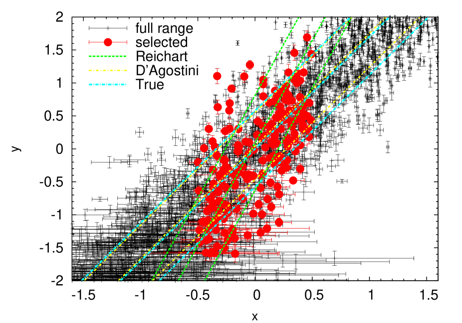
Figure 10: Full population of 1000 simulated points (crosses) from Case a, with $m_{\rm true}=1.7$ and $\sigma_{x,{\rm true}}=0.34$. Filled red circles show the selected subsample of 200 points $-0.5<x<0.5$, both fitting methods have been applied to in Case a.

5 Discussion

The results obtained from the numerical simulations show that, when the sample variance $\sigma_{x,{\rm true}}^{2}$ is significantly lower than the total variance $\sigma_{x,t}^{2}$, both methods provide a consistent estimate of the $m$ slope. Differently, when $\sigma_{x,{\rm true}}^{2}$ is comparable with $\sigma_{x,t}^{2}$, the Reichart method overestimates $m$, while the D’Agostini method still gives an estimate of $m$ compatible with the correct value $m_{\rm true}$.

The simulations have been performed adopting the same distributions of intrinsic errors along both axes, {$\sigma_{x,i}$} and {$\sigma_{y,i}$} $(i=1,\ldots,N)$, as those of the sample of 32 GRBs of GFM05. For each simulated data set, we selected 200 points within the range $-0.5<x<0.5$, similarly to the range covered in $\log{(V/\bar{V})}$ by the 32 GRBs of GFM05. Typical values of the total scatter $\sigma_{x,t}$ for the simulated data sets are 0.28–0.29, to be compared with that of the 32 GRBs of GFM05, which is 0.32. The results obtained are confirmed even when we adopt the same extrinsic scatter and 10 times smaller intrinsic errors along either axis. The most important factor is the ratio between the extrinsic scatter, $\sigma_{x,{\rm true}}$, and the total scatter, $\sigma_{x,t}$.

The two methods differ when the range along $x$ is comparable with the extrinsic scatter along the same axis. This is shown in Fig. 10: the full population clearly follows the true slope of $m_{\rm true}=1.7$ shown by the cyan line. However the two methods, applied to the 200 points selected in the range $-0.5<x<0.5$, for which the ratio $\sigma_{x,{\rm true}}/\sigma_{x,t}=0.84$, give different results, the Reichart method (green) overestimating $m$, while the D’Agostini method (yellow) is still consistent with the true slope. We do not know yet whether the $V-L$ correlation presently known extends along $V$ over a wider range, the samples considered by Reichart et al. (2001) and GFM05 being the result of truncation effects, or it does not. Either way, however, the total variance is comparable with the extrinsic variance of the correlation and in this case, the D’Agostini method turns out to be a more reliable estimator of $m$ than the Reichart.

Similar results to those presented here and by GFM05 and G05, i.e. values of $m$ around 1–2, have already been mentioned by Lloyd-Ronning et al. (2002): in fact, therein we read that a more recent analysis by Fenimore & Ramirez-Ruiz (2000) making use of a different definition of variability, based on a different degree of smoothing of the light curve, led to an estimate of $m=1.57\pm\sim 0.5$. This supports the view of a not well established value of power-law index of the $V-L$ correlation, affected by a significant scatter (Lloyd-Ronning et al., 2002).

In another recent paper by Li & Paczynski (2006) a new definition of variability is considered, based on a different smoothing filter of the light curves. In this work, they find a slope of $\sim$3, applying the fitexy procedure, and no extra variance is needed, as the correlation appears to be tight enough. These results as well as the recent analysis by Fenimore & Ramirez-Ruiz (2000) point to a strong dependence of $m$ on the kind of filter adopted to obtain a smoothed version of the light curve, with respect to which variability of the original light curve is computed.

As far as the definition of variability introduced by Reichart et al. (2001) is regarded, we have investigated reasons for the overestimation of $m$ given by the Reichart method and found that this is likely an incorrect derivation of the likelihood function by Reichart (2001) (eq. 2). This function was derived by integrating the weighted product of Gaussian density functions over, among other variables, the element $ds^{2}=(dx^{2}+dy^{2})$ (eq. 28 of Reichart 2001), where $y=y_{c}(x,\theta_{m})$ is the equation which describes the relation between the parameters $x$ and $y$ (see Section 2). The integration over $ds^{2}=(dx^{2}+dy^{2})$ is not correct: $dy$ is homogeneous with $m\,dx$ and not with just $dx$. The integration on $ds$ introduces the sum $1+m^{2}$ in the numerator of the first term at right hand side of eq. 4, which is the only difference between the likelihood functions of the two methods. The inconsistency of the term $ds$ mentioned above is transmitted to the factor $1+m^{2}$: $m$ cannot be added to 1 tout court for the same reason explained above and discussed by D’Agostini (2005). The effect of this factor is the overestimation of $m$. This is shown by the fact that, by deleting $m^{2}$, the estimate of $m$ becomes consistent and the resulting likelihood function becomes coincident with that derived by D’Agostini (2005) for the same statistical inference problem, reported here in eq. 5.

The procedure adopted by GFM05 and G05 as well as the usage of the fitexy procedure reported in Table 1 does not take into account the sample or extrinsic variance. As a result they find a high $\chi^{2}$ assuming a straight line for the correlation between $\log L$ and $\log V$. However, if, in spite of that, a straight line is assumed, the line slope $m$ value found is very close to the true one.

We conclude that the results reported by R01 and RN05, who applied the Reichart method, give an overestimated index $m$ of the power law ($L\propto V^{m}$) function used to describe the correlation between peak luminosity and variability of the GRBs included in the sample of R01, GFM05 and G05. We ascribe the different results obtained with the D’Agostini and Reichart methods, when applied to the samples of 32 GRBs of GFM05 and 551 GRBs of G05, to the comparable total variance $\sigma_{x,t}^{2}$ and extrinsic variance $\sigma_{x}^{2}$. The D’Agostini method appears to provide the most correct estimations of the slope and extrinsic scatter of either sample. The best-fitting power laws derived by GFM05 and G05 are more consistent with the results of the D’Agostini than with the Reichart method.

The implications of different power-law index and extrinsic scatter describing the $V-L$ correlation are twofold: the physical interpretation and its usage as a luminosity estimator.

5.1 Implications on the interpretation

Variability in the GRB light curves is thought to be produced mainly above the photospheric radius at which the relativistic outflow becomes optically thin to electron scattering. In addition to this photosphere, there would be a second photospheric radius beyond which shocks are optically thin to pairs too and highly variable light curves originate. Mészáros et al. (2002) interpreted the $V-L$ correlation as due to the effects of this pair-forming photosphere and the jet opening and/or viewing angles, when breaks are observed in the optical consistent with the jet interpretation. The power-law $m$ derived by those authors is $m=6p/(5q-2p)$, where they assumed $L\propto\theta^{-p}$, $p\sim 2-2.5$ ($\theta$ can be either the jet opening angle or the viewing angle for a universal jet pattern), $\Gamma_{m}\propto\theta^{-q}$ ($\Gamma_{m}$ is the minimum value of the Lorentz factor distribution of the shells). Following Mészáros et al. (2002), if one takes $p=q$, the expected power-law index is $m=2$, which is consistent within 90% CL with the value we derived with the D’Agostini method. Mészáros et al. (2002) assumed $p=5/2$ and $q=2$ to explain the value originally found by Reichart et al. (2001) and by Fenimore & Ramirez-Ruiz (2000) of $m\sim 3$. Kobayashi et al. (2002) started from similar assumptions: $\Gamma\propto\theta^{-q}$, i.e. a wider jet has a lower Lorentz factor, equal mass colliding shells, a uniform $D/c$ distribution in logarithmic spaces in the interval 1 ms–1 s ($D$ is the separation between shells). Using a simplified version of the Reichart et al. (2001) variability they tried to reproduce the $V-L$ correlation with numerical simulations and found that $q=1$ seems to better account for $m$ values in the range of 3–4, as found by Reichart et al. (2001) and Fenimore & Ramirez-Ruiz (2000). However, from the same numerical results it turns out that smaller values of $m$, compatible with the results obtained with the D’Agostini method, are given by assuming $q=2$. As already pointed out by Kobayashi et al. (2002), this is more consistent with the value $q=8/3$ derived by Salmonson & Galama (2002), based on the study of the anticorrelation between peak luminosity and jet break time. From the results of Kobayashi et al. (2002), we infer that the results of the D’Agostini best-fitting parameter $m$ imply a stronger dependence of the Lorentz factor on the opening angle as well as a smaller Lorentz factor normalisation.

Likewise, Ramirez-Ruiz & Lloyd-Ronning (2002) studied the effects of varying the energy per unit solid angle in the collimated outflow on the correlations between variability, peak luminosity and spectral peak energy (Lloyd-Ronning & Ramirez-Ruiz, 2002). They found that these correlations are accounted for if luminosity per unit solid angle $L(\theta)$ (where $\theta$ can be either the viewing angle for a structured jet pattern or the jet opening angle), strongly depends on the Lorentz factor $\Gamma(\theta)$. while the effect of changes in the baryon loading of the wind is less relevant, as it does not account for the range of variability observed. In their figure 3, Ramirez-Ruiz & Lloyd-Ronning (2002) show the results in the $V-L$ space of some numerical simulations for different bulk Lorentz factors: values for $m$ in the range 1.5–2, i.e. like those found by GFM05 and those derived in this work with the D’Agostini method, are clearly compatible with the results of these simulations.

The smaller value of $m$ we found with the D’Agostini method than with the Reichart constrains differently the parameters $m$ depends on. Moreover, the bigger extrinsic scatter of $\sigma_{\log{V}}$, 0.34 with the D’Agostini, 0.24 with the Reichart method, means a bigger scatter in the distribution of some of these parameters.

5.2 Implications on its usage as luminosity estimator

After the discovery of the $V-L$ correlation by Fenimore & Ramirez-Ruiz (2000) and Reichart et al. (2001), a number of papers used it as a luminosity estimator for several studies. Fenimore & Ramirez-Ruiz (2000) applied it to derive the luminosity distribution $\phi(L)$ and the GRB formation rate as a function of redshift $\rho(z)$. Lloyd-Ronning et al. (2002) studied the bivariate distribution of luminosity and redshift $\Psi(L,z)$ using the pseudo-redshifts obtained from a parametrisation of the $V-L$ correlation with $m=1.57\pm\sim 0.5$. They found a correlation between luminosity and redshift parametrised as $L\propto(1+z)^{1.7\pm 0.4}$. Different values of $m$ from $\sim 1$ to $\sim 3$ do not change their results qualitatively (Lloyd-Ronning et al., 2002).

Lazzati (2002) exploited the $V-L$ correlation to study the rest-frame power spectral density (PSD) in time domain for hundreds of BATSE bursts. In particular, the goal was to study the effect of photon scattering on variability. A correlation between the break frequency in the rest-frame PSD and variability was found, based on $m\sim 3$. A smaller value of $m$ would mean that a GRB with a given variability, whose dependence on $z$ is small, would be less luminous, i.e. nearer, thus with a corresponding smaller break frequency in the rest-frame PSD. This relation would have to be rescaled consequently.

More recently, other tighter correlations became popular, such as between the rest-frame peak energy $E_{\rm p}$ and the isotropic-equivalent gamma-ray released energy $E_{\gamma,{\rm iso}}$, $E_{\rm p}\propto E_{\gamma,{\rm iso}}^{0.5}$ (Amati et al., 2002), between $E_{\rm p}$ and the collimation-corrected gamma-ray released energy $E_{\gamma}$, $E_{\rm p}\propto E_{\gamma}^{0.7}$ (Ghirlanda et al., 2004). Another relation between $E_{\rm p}$, $E_{\gamma,{\rm iso}}$ and the rest-frame break time $t_{\rm b}$ of the optical afterglow light curve has been discovered recently (Liang & Zhang, 2005), which requires fewer assumptions than those of the Ghirlanda relationship. The same relation as the Amati holds with the same index of $\sim$0.5 when $E_{\gamma,{\rm iso}}$ is replaced by the peak luminosity $L_{\gamma,{\rm iso}}$, or simply $L$ (Yonetoku et al., 2004; Ghirlanda et al., 2005). Recently, the Amati relation has been confirmed for a sample of 53 long GRBs and a fit with the D’Agostini method gives an extrinsic logarithmic scatter of 0.15 over 3 orders of magnitude over $E_{\rm p}$ (Amati, 2006). In this case both methods give compatible results and this is consistent with the fact that $\sigma_{x}<<\sigma_{x,t}$. Summing up, in the case of the Amati relation, truncation effects are negligible.

Interestingly, Lloyd-Ronning & Ramirez-Ruiz (2002) studied the correlation between $V$ and $E_{\rm p}$ before the discovery of the Amati relationship. Assuming different alternative values for $m$, ranging from 2.2 to 5.8, as originally found by Fenimore & Ramirez-Ruiz (2000), they found a correlation, $E_{\rm p}\propto V^{\delta}$, with $\delta$ ranging from 0.4 to 1.15 . The Amati relation, whose extrinsic scatter is small with respect to that of the $V-L$ correlation, is more reliable as a luminosity estimator. Hence, from the Amati relation we should expect $m=\delta/0.5$, so in the range 0.8–2.3, which is consistent with the results of the D’Agostini method as well as those of GFM05 and G05.

6 Conclusions

We applied both Reichart and D’Agostini methods to the samples of 32 GRBs with known redshift and 551 BATSE GRBs with pseudo-redshift considered by GFM05 and G05, respectively. The goal was to estimate the slope $m$ as well as the scatter of the power law describing the correlation between variability and peak luminosity originally presented by Reichart et al. (2001). Both methods account for an extra variance in addition to the intrinsic affecting each single point. From simulations, we found that when the sample variance $\sigma_{x}^{2}$ is comparable with the total scatter along the same axis, $\sigma_{x,t}^{2}$, the Reichart method tends to overestimate $m$, while the D’Agostini still estimates it correctly. When the sample variance is negligible with respect to the total variance, the two methods give consistent results. In the specific case of the $V-L$ correlation, the two variances are comparable: in the case of the 32 GRBs of GFM05, it is $\sigma_{x,t}=0.32$, $\sigma_{x}=0.24$ (Reichart) or $\sigma_{x}=0.34$ (D’Agostini). This explains the discrepancy between the two methods. We showed that the D’Agostini method is a reliable estimator of $m$ in this regime, whereas the Reichart is no more. In particular, the best-fitting value for $m$ obtained with the D’Agostini method is $1.7\pm 0.4$ and $0.88_{-0.13}^{+0.12}$ at 90% confidence level for the 32 GRBs of GFM05 and for the 551 GRBs of G05, respectively. These values are significantly smaller than those obtained with the Reichart method, which are consistent with previous results of R01 and RN05. These results hold as far as the definition of variability given by R01 is assumed.

Alternatively, from other definitions of variability based on different kinds of filter used to smooth the light curves, it seems to be possible to obtain a range of values for $m$ from $\sim$1 to $\sim$3 (Fenimore & Ramirez-Ruiz, 2000; Li & Paczynski, 2006).

One of the possible implications of a smaller value of $m$ than originally found by R01 on the interpretation of the $V-L$ correlation is that, in the jet emission scenario, we would expect a stronger dependence of the Lorentz factor of the expanding shells on the jet opening angle (Kobayashi et al., 2002).

Finally, other more recent and tighter correlations, such as the Amati, Ghirlanda, Liang & Zhang relations appear to be more reliable luminosity estimators than the $V-L$ one. In particular, our results of values of $m$ in the interval 1–2 obtained with the D’Agostini method, appear to be consistent with two independent relations: $E_{\rm p}\propto V^{\delta}$ ($0.4<\delta<1.15$) (Lloyd-Ronning & Ramirez-Ruiz, 2002), and the equivalent version of the Amati relation with the isotropic-equivalent peak luminosity instead of the isotropic-equivalent total released energy, $E_{\rm p}\propto L^{0.5}$. By combining the two, one expects $m=\delta/0.5$, in agreement with the results reported here as well as those reported by GFM05 and G05.

Finally, the increasing number of GRBs with spectroscopic redshift detected by Swift (Gehrels et al., 2004) will help extend the range in $V$ and better constrain the power-law fit of the $V-L$ correlation, with the benefit of a homogeneous data set of light curves all detected with the Burst Alert Telescope (BAT) onboard Swift. A thorough test of the $V-L$ correlation with BAT data is in progress (Rizzuto et al., in preparation).

References

- Amati et al. (2002) Amati L. et al., 2002, A&A, 390, 81
- Amati (2006) Amati L., 2006, MNRAS, submitted (astro-ph/0601553)
- Band et al. (2004) Band D.L., Norris J.P., Bonnell J.T., 2004, ApJ, 613, 484
- D’Agostini (2003) D’Agostini G., 2003, Bayesan reasoning in data analysis: A critical Introduction, World Scientific Publishing.
- D’Agostini (2005) D’Agostini G., 2005, physics/0511182
- Fenimore & Ramirez-Ruiz (2000) Fenimore E.E., Ramirez-Ruiz E., 2000, astro-ph/0004176
- Gehrels et al. (2004) Gehrels N. et al., 2004, ApJ, 611, 1005
- Ghirlanda et al. (2004) Ghirlanda G., Ghisellini G. & Lazzati D., 2004, ApJ, 616, 331
- Ghirlanda et al. (2005) Ghirlanda G., Ghisellini G., Firmani C., Celotti A. & Bosnjak Z., 2005, MNRAS, 360, L45
- Guidorzi et al. (2005) Guidorzi C., Frontera F., Montanari E., Rossi F., Amati L., Gomboc A., Hurley K., Mundell C.G., 2005, MNRAS, 363, 315 (GFM05)
- Guidorzi (2005) Guidorzi C., 2005, MNRAS, 364, 163 (G05)
- Haislip et al. (2006) Haislip J.B. et al., 2006, Nature, 440, 181
- Kawai et al. (2006) Kawai N. et al., 2006, Nature, 440, 184
- Kobayashi et al. (2002) Kobayashi S., Ryde F. & MacFayden A., 2002, ApJ, 577, 302
- Ioka & Nakamura (2001) Ioka, K. & Nakamura, T., 2001, ApJ, 554, L163
- Lazzati (2002) Lazzati D., 2002, MNRAS, 337, 1426
- Li & Paczynski (2006) Li L. & Paczynski B., 2006, MNRAS, 366, 219
- Liang & Zhang (2005) Liang E. & Zhang B., 2005, ApJ, 633, 611
- Lloyd-Ronning et al. (2002) Lloyd-Ronning N.M., Fryer C.L. & Ramirez-Ruiz E., 2002, ApJ, 574, 554
- Lloyd-Ronning & Ramirez-Ruiz (2002) Lloyd-Ronning N.M. & Ramirez-Ruiz E., 2002, ApJ, 576, 101
- Mészáros et al. (2002) Mészáros P., Ramirez-Ruiz E., Rees M.J., & Zhang B., 2002, ApJ, 578, 812
- Nava et al. (2006) Nava L., Ghisellini G., Ghirlanda G., Tavecchio F. & Firmani C., 2006, A&A, 450, 471
- Norris et al. (2000) Norris J.P., Marani G.F., Bonnell J.T., 2000, ApJ, 534, 248
- Norris (2002) Norris J.P., 2002, ApJ, 579, 386
- Paciesas et al. (1999) Paciesas W.S. et al., 1999, ApJS, 122(2), 465
- Press et al. (1993) Press W.H., Flannery B.P., Teukolsky S.A., Vetterling W.T., 1993, Numerical Recipes in C, Cambridge University Press, 2nd edition
- Ramirez-Ruiz & Lloyd-Ronning (2002) Ramirez-Ruiz E. & Lloyd-Ronning N.M., 2002, New A, 7, 197
- Reichart et al. (2001) Reichart D.E., Lamb D.Q., Fenimore E.E., Ramirez-Ruiz E., Cline T.L., Hurley K., 2001, ApJ, 552, 57 (R01)
- Reichart (2001) Reichart D.E., 2001, ApJ, 553, 235 (RM)
- Reichart & Nysewander (2005) Reichart D.E., Nysewander M.C., 2005, ApJ, submitted (astro-ph/0508111) (RN05)
- Reichart (2005) Reichart D.E., 2005, astro-ph/0508529
- Salmonson & Galama (2002) Salmonson J.D. & Galama T.J., 2002, ApJ, 569, 682
- Yonetoku et al. (2004) Yonetoku D., Murakami T., Nakamura T., Yamazaki R., Inoue A.K. & Ioka K., 2004, ApJ, 609, 935