Interacting models of soft coincidence

Abstract

The coincidence problem of late cosmic acceleration is a serious riddle in connection with our understanding of the evolution of the Universe. In this paper we show that an interaction between the dark energy component (either phantom or quintessence) and dark matter can alleviate it. In this scenario the baryon component is independently conserved. This generalizes a previous study [S. del Campo, R. Herrera, and D. Pavón, Phys. Rev. D 71, 123529 (2005)] in which neither baryons nor phantom energy were considered.

I Introduction

According to the conventional picture, the present accelerated expansion of the Universe is driven by the negative pressure of an unknown and unclustered component (dubbed “dark energy”) that currently contributes about $70$% of the total density. The remaining $30$ per cent is shared between cold dark matter ($\rho_{dm}\sim 25$%) and cold baryons ($\rho_{b}\sim 5$%) accel ; wmap ; hzt ; snls ; wmap3y . The two latter, being pressureless, redshift with expansion faster than the dark energy component. Then, the cosmic coincidence problem arises, “Why are the densities of matter and dark energy of precisely the same order today?” coincidence . Clearly, this is one outstanding riddle in our understanding of the Universe. To solve it one is forced to adopt an evolving dark energy field (either quintessence or phantom energy) or accept an incredibly tiny cosmological constant and admit that the “coincidence” is just a coincidence that hopefully might be somewhat alleviated with the help of the anthropic idea reviews . Here we take the view that before resorting to the second option we should further explore the first one. Yet, an evolving dark energy cannot solve the problem either unless a suitable interaction (coupling) with matter is allowed interaction ; recent . Note that the coupling alters the rate at which both matter and dark energy redshift with expansion; this is why it can potentially alleviate the aforesaid problem.

Interestingly, rather than in connection with the coincidence problem, which was not even formulated at the moment, this interaction was first proposed as a mechanism to reduce the value of the cosmological constant wetterich . Notice that in the absence of underlying symmetry that would suppress the coupling matter–dark energy there is no a priori reason to dismiss it. In the last years, various proposals at the fundamental level for the coupling leading to a constant ratio matter/dark energy at late times were advanced (see e.g., federico and references therein), and specific phenomenological models have been built and contrasted with observational data (high redshift supernovae and CMB anisotropies) and seen to pass the tests tests . Further, the Akaike akaike and Bayesian informative criteria bic when applied to high redshift supernovae data suggest a transfer of energy from the phantom component to the matter component; yet, the conventional $\Lambda$CDM model is still preferred szydlowsky .

While a constant ratio matter/dark–energy at late times (including the present one) would clearly alleviate the coincidence problem it should be noted that a much less strong condition would serve. It would suffice that nowadays the aforesaid ratio varies only slowly (i.e., less faster than the scale factor) and be of order unity (“soft coincidence”). Recently, it was found within this approach that the quintessence scenario was favored over the tachyon scenario for the latter would imply an excessive amount of pressureless matter today recent . However, in order to circumvent the tight constraints on long–range forces tight the baryon component was left aside altogether. This may be justified because the analysis was restricted to times about the present one which, as said above, is characterized, among other things, by a low value to the baryon density. In this paper we generalize the analysis by including baryons in the energy density budget as an independently conserved component and extend the study to earlier times -though not to the radiation dominated era. As dark energy components quintessence and phantom are separately considered.

The outline of the paper is as follows. In section II we present the model. In section III we constrain it with recent high redshift supernovae data. Finally, in section IV we discuss and summarize our findings. As usual, a zero subscript or superscript attached to any quantity means that it should be evaluated at the present epoch.

II The interacting model

We consider a spatially flat Friedmann-Lemaitre-Robertson-Walker universe dominated by a three-component system, namely, cold baryonic matter, cold non-baryonic dark matter and dark energy, such that the two latter components do not conserve separately but interact with each other in a manner to be specified below. The energy density and pressure of the dark energy, assuming it is a quintessence field, are given by

$$\rho_{\phi}=\textstyle{1\over{2}}\dot{\phi}^{2}+V(\phi)\,,\qquad\mbox{and}\qquad P_{\phi}=\textstyle{1\over{2}}\ \dot{\phi}^{2}-V(\phi),$$ (1)

respectively. If the dark energy is a phantom field we have instead,

$$\rho_{\phi}=-\textstyle{1\over{2}}\dot{\phi}^{2}+V(\phi)\,,\qquad\mbox{and}\qquad P_{\phi}=-\textstyle{1\over{2}}\ \dot{\phi}^{2}-V(\phi).$$ (2)

The upper-dot stands for derivative with respect to the cosmic time and $V(\phi)$ denotes both the quintessence field potential and phantom potential. As is usually done, we postulate that the dark energy component (either quintessence or phantom) obeys a barotropic equation of state, i.e., $P_{\phi}=w_{\phi}\,\rho_{\phi}$ with $w_{\phi}$ a negative constant of order unity (a distinguishing feature of dark energy fields is a high negative pressure).

We assume that the dark matter and dark energy components are coupled through a source (loss) term (say, $Q$) that enters the energy balances

$$\dot{\rho}_{dm}+3H\rho_{dm}=Q,$$ (3)

and

$$\dot{\rho}_{\phi}+3H(\rho_{\phi}+P_{\phi})=-Q\,.$$ (4)

In view of Eq.(1) last expression can alternatively be written as $\dot{\phi}\left[\ddot{\phi}+3H\dot{\phi}+V^{\prime}\right]=-Q$. In the case that the scalar field is of phantom type the corresponding equation reads $\dot{\phi}\left[\ddot{\phi}+3H\dot{\phi}-V^{\prime}\right]=Q$, where the prime denotes derivative with respect to $\phi$.

We consider that the baryon component is conserved whence its energy density redshifts as

$$\rho_{b}=\rho_{b}^{0}\left(\frac{a_{0}}{a}\right)^{3}.$$ (5)

Defining $\rho_{m}=\rho_{b}+\rho_{dm}$ and using Eqs.(3) and (5) we obtain

$$\dot{\rho}_{m}+3H\rho_{m}=Q.$$ (6)

Likewise, we assume that the interaction is related to the total energy density of matter (baryonic plus dark) by $Q=3c^{2}H\rho_{m}$, where $c^{2}$ is a small positive–definite constant. As we shall see this choice ensures that the ratio between the energy densities, $r(a)\equiv\rho_{m}/\rho_{\phi}$, is a monotonous decreasing function of the scale factor, and such that around present time it varies very slowly. By very slowly we mean that $\mid(\dot{r}/r)_{0}\mid\lesssim H_{0}$. This contrasts with previous studies in which $r$ was demanded to asymptotically approach a fixed value at late times.

Clearly,

$$\dot{r}\equiv\frac{d}{dt}\left[\frac{\rho_{m}}{\rho_{\phi}}\right]=\frac{\rho_{m}}{\rho_{\phi}}\left(\frac{\dot{\rho}_{m}}{\rho_{m}}-\frac{\dot{\rho}_{\phi}}{\rho_{\phi}}\right).$$ (7)

In virtue of the above expressions last equation boils down to

$$\dot{r}=3Hr\left[c^{2}(1+r)-|w_{\phi}|\right]\,,$$ (8)

whose solution reads

$$r=r_{0}\,\xi\left[c^{2}r_{0}-\left(\frac{a}{a_{0}}\right)^{3\xi}[c^{2}(1+r_{0})-|w_{\phi}|]\right]^{-1},$$ (9)

with $\xi\equiv|w_{\phi}|-c^{2}>0$. Figure 1 depicts the monotonous decrease of $r$ from values higher than unity at early times to a nearly constant value at present time (which we have fixed as $3/7$) irrespective of whether the dark energy is a quintessence field or a phantom field. Notice that for vanishing scale factor $r$ tends to the finite, constant value $\xi/c^{2}$. However, our model should not be extrapolated to such early stage.

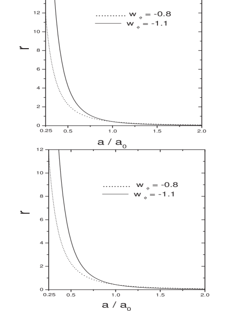
Figure 1: Evolution of the ratio $\rho_{m}/\rho_{\phi}$ as given by Eq.(9) for $c^{2}=10^{-5}$ (upper panel) and $c^{2}=10^{-3}$ (lower panel). In both panels $r_{0}=3/7$ with $w_{\phi}=-0.8$ (quintessence) and $w_{\phi}=-1.1$ (phantom). Not shown is the behavior of $r$ for $a\rightarrow 0$ as the model does not apply to such early times.

One may wonder about the size of $c^{2}$. Obviously it should not be large. In any case it must be lower than $|w_{\phi}|/(1+r_{0})$; otherwise, by Eq. (8), the Universe would have been dominated by the dark energy from the beginning of the expansion and galaxies would not have come into existence. On the other hand, it should not be very small for it would have a negligible impact and our model would be hardly distinguishable (depending on the value of $w_{\phi}$) from the standard quintessence or phantom models.

Because of $c^{2}$ ought to be a small quantity -though not very small-, the right hand side of Eq.(9) always stays above zero, becoming negligible only for $a\gg a_{0}$. The closer $c^{2}$ is to $|w_{\phi}|/(1+r_{0})$, the more alleviated the coincidence problem gets. In particular, for $c^{2}>[\mid w_{\phi}\mid-1/3](1+r_{0})^{-1}$ the current rate, $\mid(\dot{r}/r)_{0}\mid$, results lower than $H_{0}$ (bear in mind that the corresponding rate in case the dark energy were just the cosmological constant is $3H_{0}$), whereby the criterion of “soft coincidence” is satisfied and the coincidence problem gets significantly alleviated.

From Eq.(6) along with the expression for $Q$ we get

$$\rho_{m}=\rho_{m}^{0}\;\left(\frac{a_{0}}{a}\right)^{3(1-c^{2})}\,.$$ (10)

Thus, the densities of dark matter and dark energy are given by

$$\rho_{dm}=\left(\frac{a_{0}}{a}\right)^{3}\left[\rho_{m}^{0}\left(\frac{a_{0}}{a}\right)^{-3c^{2}}-\rho_{b}^{0}\right],$$ (11)

and

$$\rho_{\phi}=\frac{\rho_{m}^{0}}{r_{0}\xi}\left(\frac{a_{0}}{a}\right)^{3(1-c^{2})}\left[c^{2}r_{0}-\left(\frac{a}{a_{0}}\right)^{3\xi}[c^{2}(1+r_{0})-|w_{\phi}|]\right]\,,$$ (12)

respectively. Obviously, the constant $c^{2}$ could be determined if either $\rho_{m}$, given by Eq. (10) above, or the ratio $\rho_{b}/\rho_{m}\propto a^{-3c^{2}}$, were accurately known at different redshifts. The above expression for $\rho_{dm}$ may suggest that this quantity becomes negative at small scale factor. That is so; however, if one takes into account that $\rho^{0}_{b}/\rho^{0}_{m}$ is about $0.2$, for reasonable values of $c^{2}$, this only occur well in the radiation era, i.e., beyond the range of applicability of our model.

As Fig. 1 shows, $r\geq 10$ at sufficiently early times (e.g., at redshifts larger than, say, $3$). This is consistent with the analysis of Caldwell et al. earlyq who found that at the epoch of last scattering ($z\simeq 1,100$) as well as at the onset of structure formation ($z\sim 10^{3}$) $\Omega_{\phi}$ (the energy density of the dark energy in units of the critical density) should not exceed $0.1$.

On the other hand, from Eqs. (3) and (5) alongside the condition $Q>0$ it follows that the baryon density never dominates the matter density (i.e., $\rho_{b}/\rho_{dm}<1$ always). This is in keeping with the widely accepted scenario of cosmic structure formation, in which after the last scattering the baryonic matter freely fells into the deep potential wells created by the dark matter. If $\rho_{b}$ were larger than $\rho_{dm}$ at early times, then the aforesaid scenario could be spoiled.

By combining Friedmann’s equation

$$3H^{2}=\kappa(\rho_{b}+\rho_{dm}+\rho_{\phi})\quad\qquad(\kappa\equiv 8\pi\,G),$$ (13)

with Eqs. (10)–(12) we get the Hubble function

$$H(a)=\frac{H_{0}}{\sqrt{(1+r_{0})\xi}}\,\left(\frac{a_{0}}{a}\right)^{\frac{3}{2}(1-c^{2})}\left[|w_{\phi}|\,r_{0}-\left(\frac{a}{a_{0}}\right)^{3\xi}[c^{2}(1+r_{0})-|w_{\phi}|]\right]^{1/2},$$ (14)

where $H_{0}=\sqrt{(1+r_{0})\kappa\,\rho_{\phi}^{0}/3}$, which will be needed below both to obtain the luminosity distance -a previous step to draw the likelihood contours- and the deceleration parameter, $q=-\ddot{a}/(aH^{2})$. The evolution of the latter as a function of the redshift is depicted in Fig. 2.

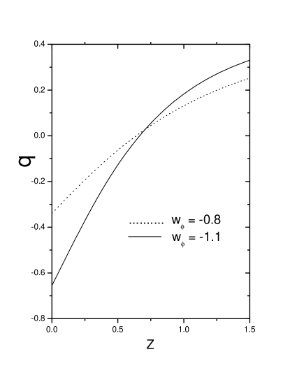
Figure 2: The deceleration parameter as a function of the redshift, $z=(a_{0}/a)-1$. Here $r_{0}=3/7$ and $c^{2}=10^{-3}$.

In this model the universe began accelerating only recently, at redshifts about $0.65$. As we have checked numerically this behavior is scarcely sensitive to the value of the $c^{2}$ parameter provided this lies in the range $10^{-5}\leq c^{2}\leq 10^{-1}$ (this is why we content ourselves with presenting just two plots of $q$ vs. $z$). The larger $c^{2}$, the larger the transition redshift.

Using Eq.(1) (respectively, Eq.(2)) the potential for the quintessence field (respectively, phantom field) in terms of the scale factor reads

$$V(\phi(a))=(1+|w_{\phi}|)\;\frac{\rho_{m}^{0}}{2r_{0}\xi}\left(\frac{a_{0}}{a}\right)^{3(1-c^{2})}\left[c^{2}r_{0}-\left(\frac{a}{a_{0}}\right)^{3\xi}[c^{2}(1+r_{0})-|w_{\phi}|]\right].$$ (15)

To obtain the potential as a function of $\phi$ we must first express the latter in terms of $a$. To this end, we write

$$\dot{\phi}^{2}=\pm\left(\frac{d\phi}{da}\,H\,a\right)^{2},$$ (16)

where the plus(minus) sign corresponds to quintessence field (phantom field). And in virtue of Eqs. (12), (13) and (16) it follows that

$$\phi-\phi_{0}=\sqrt{\frac{\pm 3(1-|w_{\phi}|)}{\kappa}}\;\frac{1}{3\xi}\;\left[\left(\ln\Im(a)+\frac{c}{\sqrt{|w_{\phi}|}}\ln\Re(a)\right)-C\right],$$ (17)

where

$$\Im(a)=-c^{2}r_{0}+2c^{2}(a/a_{0})^{3\xi}(1+r_{0})-(r_{0}+2(a/a_{0})^{3\xi})|w_{\phi}|$$

$$+2\sqrt{|w_{\phi}|(a/a_{0})^{3\xi}-c^{2}((a/a_{0})^{3\xi}+r_{0}[(a/a_{0})^{3\xi}-1])}\,\sqrt{|w_{\phi}|(r_{0}+(a/a_{0})^{3\xi})-c^{2}(1+r_{0})(a/a_{0})^{3\xi}}\,,$$

$$\Re(a)=\frac{-3\xi(a/a_{0})^{-3\xi}}{c^{3}r_{0}\sqrt{|w_{\phi}|}}\;\;\left[\;c^{4}(1+r_{0})(a/a_{0})^{3\xi}+c^{2}r_{0}|w_{\phi}|[(a/a_{0})^{3\xi}-2]-w_{\phi}^{2}(a/a_{0})^{3\xi}\right.$$

$$-2c\sqrt{|w_{\phi}|}\,\sqrt{|w_{\phi}|(a/a_{0})^{3\xi}-c^{2}[(a/a_{0})^{3\xi}+r_{0}((a/a_{0})^{3\xi}-1)]}$$

$$\times\;\left.\sqrt{(r_{0}+(a/a_{0})^{3\xi})|w_{\phi}|-c^{2}(1+r_{0})(a/a_{0})^{3\xi}}\right]\,,$$

and $C$ denotes the integration constant

$$C=\ln\Im(a_{0})+\sqrt{\frac{c^{2}}{|w_{\phi}|}}\,\ln\Re(a_{0})\,.$$

The dependence of the potential on the field $\phi$ is shown in Fig. 3.

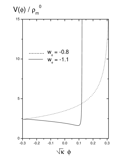
Figure 3: The normalized potential, $V(\phi)/\rho^{0}_{m}$, vs $\sqrt{\kappa}\phi$. Here $r_{0}=3/7$, $c^{2}=10^{-3}$ and $\phi_{0}=(C/3\xi)\;\sqrt{\pm 3(1-|w_{\phi}|)/\kappa}$, the plus (minus) sign corresponds to the quintessence field (phantom field).

Clearly, this potential must be understood as an effective one. It should be noted that these effective potentials (quintessence and phantom potentials) are similar to those used in inflationary models, where the universe undergoes an accelerated period at very early times. Thus, our potentials describe an accelerated phase at present time, and simultaneously alleviate the coincidence problem.

III Comparing with supernovae data

In this section we use two independent supernovae type Ia (SNIa) data sets, namely the “gold” sample compiled by the High-Z Supernovae Search Team (HZT) hzt , and the Supernova Legacy Survey (SNLS) sample snls , to constrain the parameters of the model. The “gold” sample, collected from different sources, comprises $157$ SNIa, of redshifts up to $1.5$ ($14$ of which, discovered by the Hubble Space Telescope, lie in the interval $1<z<1.5$), with reduced calibration errors coming from systematics. The SNLS sample is smaller, $71$ SNIa, with redshifts below unity. However, the technique employed guarantees that no source is lost and the data are of a higher quality.

Figures 4 and 5 depict the best–fit of the phantom model (solid line) and the quintessence model (dashed line) to the “gold” sample and the SNLS sample, respectively. For the sake of comparison the flat $\Lambda$CDM model is also shown. In plotting the graphs the expression for the distance modulus, $\mu=5\log d_{L}+25$, was employed. Here $d_{L}=(1+z)\int_{0}^{z}{H^{-1}(z^{\prime})dz^{\prime}}$, is the luminosity distance in megaparsecs.

Figure 4: Distance modulus vs redshift for the best fit quintessence model, $\Omega_{\phi}=0.71$, $w_{\phi}=-0.99$, $c^{2}=10^{-5}$, $\chi^{2}=177$ (dashed line), and the phantom model, $\Omega_{\phi}=0.40$, $w_{\phi}=-4.63$, $c^{2}=0.20$, $\chi^{2}=173$ (solid line). The flat $\Lambda$CDM model is also included, $\Omega_{\Lambda}=0.70$, $w_{\Lambda}=-1$, $\chi^{2}=178$ (dotted line). The data points correspond to the “gold” sample of SNIa hzt .

Figure 5: Distance modulus vs redshift for the best fit quintessence model, $\Omega_{\phi}=0.74$, $w_{\phi}=-0.99$, $c^{2}=10^{-5}$, $\chi^{2}=111.09$ (dashed line), and the phantom model, $\Omega_{\phi}=0.70$, $w_{\phi}=-1.10$, $c^{2}=0.035$, $\chi^{2}=111.02$ (solid line). The flat $\Lambda$CDM model is also included, $\Omega_{\Lambda}=0.72$, $w_{\Lambda}=-1$, $\chi^{2}=111.03$ (dotted line). The data points correspond to the SNLS sample snls .

Figures 6 and 7 portray the two–dimensional likelihood contours for the case that the dark energy component is a quintessence field, based on the “gold” hzt and the SNLS sample snls , respectively. Both set of contours were calculated by running through a grid of models on a four-dimensional parameter space. The prior $\Omega_{m}+\Omega_{\phi}=1$ was used and the present value of the Hubble parameter was allow to vary in the interval $60<H_{0}<70\,$km/s/Mpc. The rest of the priors are $10^{-5}<c^{2}<0.3$, and $-1<w_{\phi}<-0.6$. The constraints obtained on the free parameters from the HZT data are: $\Omega_{\phi}=0.74^{+0.06}_{-0.07}$, $w_{\phi}(1\sigma)<-0.9$, $c^{2}(1\sigma)<0.13$. The latter parameter shows large degeneracy and only in this case we find an upper limit. In its turn, the constraints obtained on the free parameters from the SNLS data are: $\Omega_{\phi}=0.83^{+0.08}_{-0.09}$, $w_{\phi}(1\sigma)<-0.62$. Unfortunately, the $c^{2}$ parameter is practically not constrained in this case.

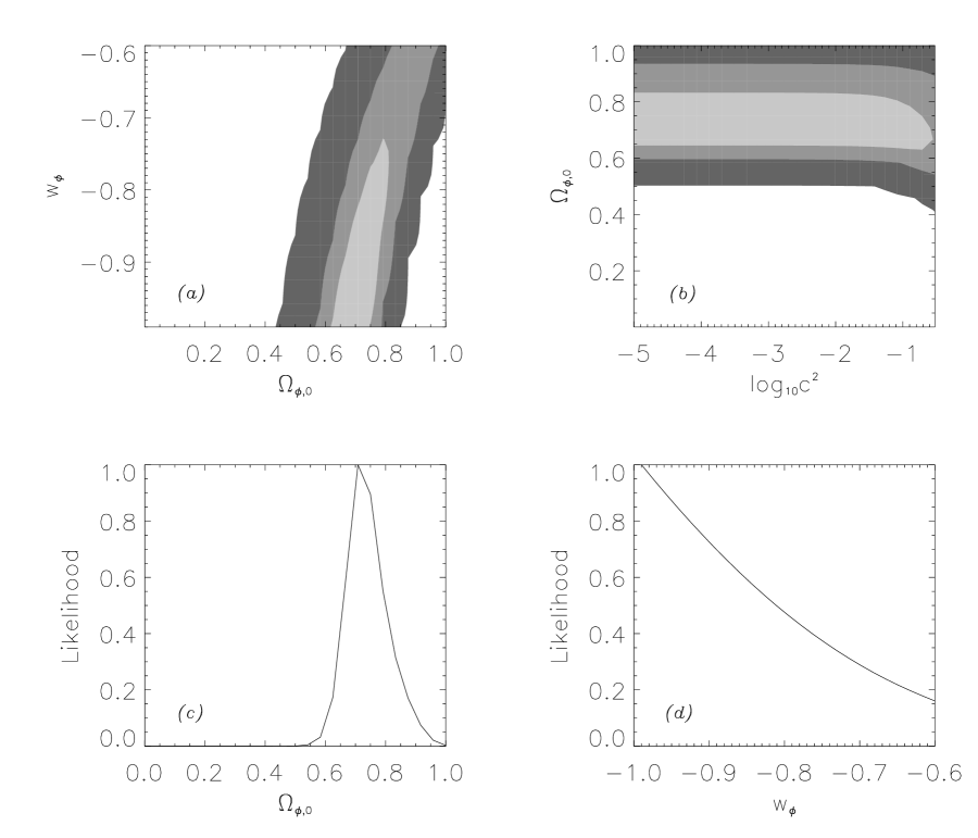
Figure 6: Likelihood contours for the quintessence model displaying the $68$%, $95$%, and $99.99$% confidence intervals. The likelihood are marginalized over the rest of the parameters. The bottom panels show the the probability functions for the quintessence energy density normalized to the critical density (left panel), and the equation of state parameter of the quintessence fluid (right panel). The data points correspond to the “gold” sample of SNIa hzt .

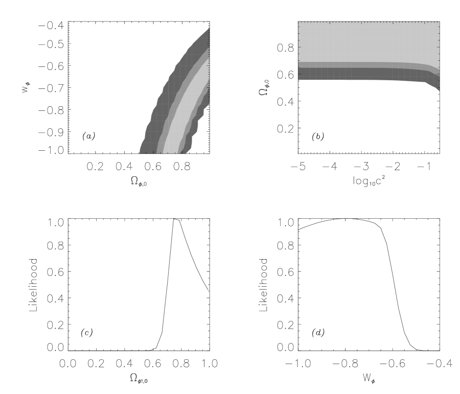
Figure 7: Same as Fig. 6 except that the data points correspond to the SNLS data set of Ref. snls .

Similarly, Figs. 8 and 9 show the corresponding contours for the phantom model using identical sets of data and the priors $10^{-5}<c^{2}<0.3$, $-5<w_{\phi}<-0.6$. The constraints obtained on the free parameters from the first set (HZT) are: $\Omega_{\phi}=0.48\pm 0.06$, $w_{\phi}=-3.0\pm 1.1$. Again, the interaction parameter $c^{2}$ shows a wide degeneracy. In its turn, the constraints obtained from the SNLS data set are: $\Omega_{\phi}=0.71^{+0.12}_{-0.13}$, $w_{\phi}=-1.1\pm 0.4$, with no real constraint on $c^{2}$ given its large degeneracy.

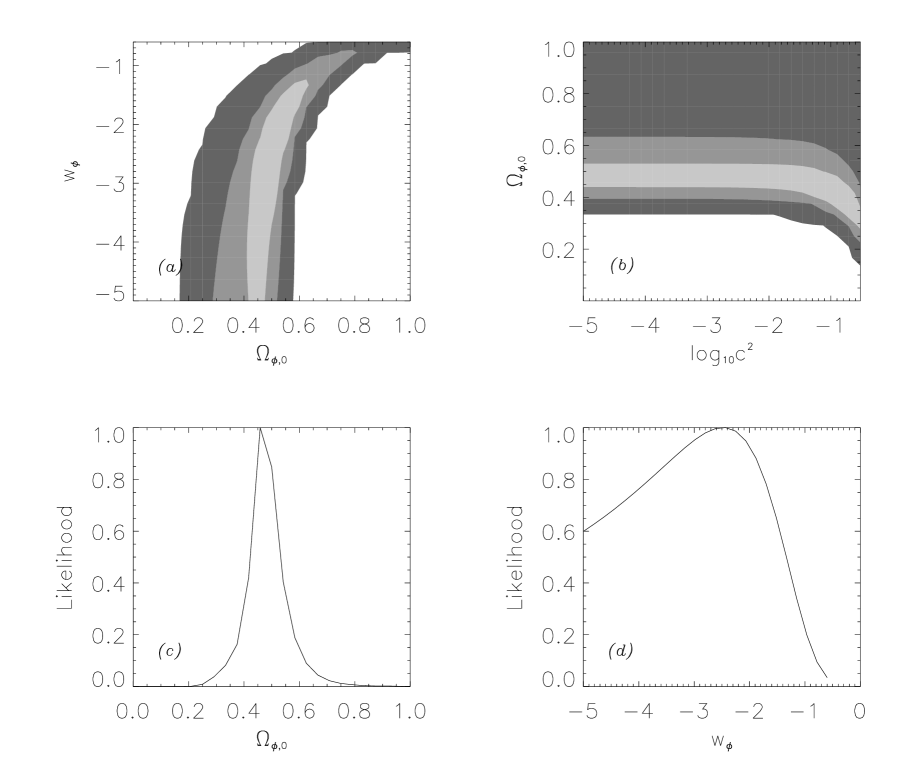
Figure 8: Likelihood contours for the phantom model displaying the $68$%, $95$%, and $99.99$% confidence intervals. The likelihood are marginalized over the rest of the parameters. The bottom panels show the the probability functions for the phantom energy density normalized to the critical density (left panel), and the equation of state parameter of the phantom fluid (right panel). The data points correspond to the “gold” sample of SNIa hzt .

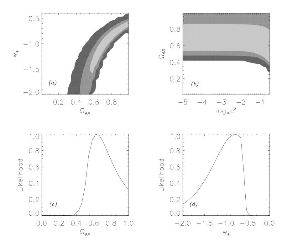
Figure 9: Same as Fig. 8 except that the data points correspond to the SNLS data set of Ref. snls .

As is usual in scenarios of late acceleration, this model prefers a lower contribution of dark energy. The fact that phantom models prefer a lower value of $\Omega_{\phi}$ is only natural given their low value of $w_{\phi}$. It interesting to see that the SNLS data favor a higher value for $\Omega_{\phi}$ (both for phantom and quintessence models) than HZT’s.

IV Discussion

We studied a model of late cosmic acceleration by assuming that the dark matter and dark energy components are coupled to each other so that there is a transfer of energy from the latter to the former, while the baryon component is conserved. By suitably choosing the interaction term, $Q$, the ratio between both dark sources of gravity is seen to evolve, at present time, less faster than the scale factor. This considerably alleviates the coincidence problem albeit it does not solve it in full. Clearly, to achieve the latter one should derive the present value of the aforesaid ratio, or at least show that it has to be of order unity. For the time being, $r_{0}$ ought to be understood as an input parameter. This also holds for a handful of key observational quantities such as the present value of the cosmic background radiation temperature, the cosmological constant $H_{0}$, or the ratio between the number of baryons and photons.

The transition deceleration–acceleration occurs recently, at redshifs lower than unity (see Fig. 2). This contrasts with other interacting models in which the transition is predicted to take place much earlier, at redshifhts as hig as $10$ transition .

It is noteworthy that the expression for the potential, Eq. (15), is identical irrespective of whether the dark energy component is a phantom or a quintessence field.

Both when the dark energy is a quintessence or a phantom field the model fits rather well the HZT data set, and in the latter case clearly better than the concordance model $\Lambda$CDM does ($\chi^{2}_{phantom}=173$, $\chi^{2}_{quintessence}=177$, $\chi^{2}_{\Lambda}=178$). Yet, the Bayesian information criterion (BIC) bic , given by the formula BIC$=\chi^{2}+p\,\ln N$, where $p$ is the number of free parameters of the model ($2$ for the $\Lambda$CDM model, $4$ for dark energy models) and $N$ the number of data points, distinctly favors the $\Lambda$CDM model for it yields a lower figure (BIC${}_{quintessence}\simeq 197$, BIC${}_{phantom}\simeq 193$, BIC${}_{\Lambda}\simeq 188$).

The fits to the SNLS data are rather similar ($\chi^{2}_{phantom}=111.02$, $\chi^{2}_{quintessence}=111.09$, $\chi^{2}_{\Lambda}=111.03$). However, the Bayesian information criterion again sides with the $\Lambda$CDM model (BIC${}_{quintessence}\simeq$ BIC${}_{phantom}\simeq 128$, BIC${}_{\Lambda}\simeq 119$).

We have not used the Akaike criterion because it favors models with larger number of parameters favors .

Thus, from the point of view of the Bayesian information criterion the $\Lambda$CDM model is preferred, and the soft coincidence model for quintessence seems clearly disfavored if not discarded. As for the phantom model, the situation appears somewhat undecided. While, regarding the BIC, it lags behind the concordance model it shows a better fit to the HZT sample of supernovae and alleviates the coincidence problem. We may summarize by saying that the SNIa data are not yet conclusive thereby a richer supernovae statistics, especially at redshifts larger than unity, is needed to come to a verdict.

Unfortunately, the supernovae constraints on the $c^{2}$ parameter is rather poor. This is coherent with the fact that the interaction dark energy–dark matter affects the luminosity distance only at third order in the redshift grg1-2 . Nevertheless, we hope to be able to break the degeneracy by submitting the model to further tests such as the CMB temperature anisotropies and the distribution of matter at cosmological scales. This will be the subject of a future work.

- (1) A.G. Riess et al., Astron. J. 116, 1009 (1998); S. Perlmutter et al., Astrophys. J. 517, 565 (1999); W.J. Percival, et al, Mon. Not. R. Astron. Soc., 327, 1297 (2001); A. Clochiatti et al., astro-ph/0510155.
- (2) D. Spergel et al., Astrophys. J. Suppl. 148, 175 (2003).
- (3) A.G. Riess et al., Astrophys. J. 607, 665 (2004).
- (4) P. Astier et al., J. Astron. Astrophys. 447, 31 (2006).
- (5) D. N. Spergel et al., astro-ph/0603449.
- (6) P.J. Steinhardt, in Critical Problems in Physics, edited by V.L. Fitch and and D.R. Marlow (Princeton University Press, Princeton, NJ, 1997).
- (7) Proceedings of the I.A.P. Conference On the Nature of Dark Energ, Paris, edited by P. Brax et al. (Frontier Groupe, Paris, 2002). Carroll, in Measuring and Modeling the Universe, Carnegie Observatories Astrophysics Series, Vol. 2, edited by W.L. Freedman (Cambridge University Press, Cambridge, 2004); V. Sahni, astro-ph/0403324; Proceedings of the Conference Where Cosmology and Fundamental Physics Meet, edited by V. Lebrun, S. Basa and A. Mazure (Frontier Group, Paris, 2004); L. Perivolaropoulos, astro-ph/0601014; E.J. Copeland, M. Sami and S. Tsujikama, hp-th/0603057.
- (8) S. del Campo, R. Herrera, and D. Pavón, Phys. Rev. D 71, 123529 (2005).
- (9) L. Amendola, Phys. Rev. D. 62, 043511 (2000); W. Zimdahl, D. Pavón, and L.P. Chimento, Phys. Lett. B 521, 133 (2001); D. Tocchini-Valentini, and L. Amendola, Phys. Rev. D 65, 063508 (2002); W. Zimdahl and D. Pavón, Gen. Rel. Grav. 35, 413 (2003); L.P. Chimento, A.S. Jakubi, D. Pavón, and W. Zimdahl, Phys. Rev. D 67, 083513 (2003); S. del Campo, R. Herrera and D. Pavón, Phys. Rev. D 70, 043540 (2004); D. Pavón, S. Sen, and W. Zimdahl, JCAP 05(2004)009; G. Farrar and P.E.J. Peebles, Astrophys. J. 604, 1 (2004) ; R-G Cai and A. Wang, JCAP 03(2005)002; D. Pavón and W. Zimdahl, Phys. Lett. B 628, 206 (2005); L.P. Chimento and D. Pavón, Phys. Rev. D 73, 063511 (2006).
- (10) C. Wetterich, Nucl. Phys. B 302, 668 (1988); C. Wetterich, Astron. Astrophys. 301, 321 (1995).
- (11) F. Piazza and S. Tsujikawa, JCAP 07(2004)004; B. Gumjudpai, T. Naskar, M. Sami, and S. Tsujikawa, JCAP 06(2005)007.
- (12) L. Amendola, M. Gasperini, and F. Piazza, JCAP 09(2004)014; G. Olivares, F. Atrio-Barandela, and D. Pavón, Phys. Rev. D 71, 063523 (2005); E. Majerotto, D. Sapone, and L. Amendola, astro-ph/0410543.
- (13) H. Akaike, IEEE Trans. Auto Control 19, 716 (1974).
- (14) G. Schwarz, Annals of Statistics 5, 461 (1978).
- (15) M. Szydlowsky, T. Stachowiak, and R. Wojtak, Phys. Rev. D 73, 063516 (2006).
- (16) K. Hagiwara et al., Phys. Rev. D 66, 010001 (2002).
- (17) R.R. Caldwell et al., Astrophys. J. Letters 591, L75 (2003).
- (18) See first and fifth papers in Ref.interaction .
- (19) See Sec. 3 of Ref. szydlowsky .
- (20) W. Zimdahl and D. Pavón, Gen. Relativ. Grav. 35, 413 (2003); 36, 1483 (2004).