The hierarchical formation of the brightest cluster galaxies

Abstract

We use semi-analytic techniques to study the formation and evolution of brightest cluster galaxies (BCGs). We show the extreme hierarchical nature of these objects and discuss the limitations of simple ways to capture their evolution. In a model where cooling flows are suppressed at late times by AGN activity, the stars of BCGs are formed very early (50 per cent at $z\sim 5$, 80 per cent at $z\sim 3$) and in many small galaxies. The high star formation rates in these high-$z$ progenitors are fuelled by rapid cooling, not by merger-triggered starbursts. We find that model BCGs assemble surprisingly late: half their final mass is typically locked-up in a single galaxy after $z\sim 0.5$. Because most of the galaxies accreted onto BCGs have little gas content and red colours, late mergers do not change the apparent age of BCGs. It is this accumulation of a large number of old stellar populations – driven mainly by the merging history of the dark matter halo itself – that yields the observed homogeneity of BCG properties. In the second part of the paper, we discuss the evolution of BCGs to high redshifts, from both observational and theoretical viewpoints. We show that our model BCGs are in qualitative agreement with high-$z$ observations. We discuss the hierarchical link between high-$z$ BCGs and their local counter-parts. We show that high-$z$ BCGs belong to the same population as the massive end of local BCG progenitors, although they are not in general the same galaxies. Similarly, high-$z$ BCGs end-up as massive galaxies in the local Universe, although only a fraction of them are actually BCGs of massive clusters.

1 Introduction

Brightest cluster galaxies (BCGs) are the very bright galaxies that inhabit the cores of rich galaxy clusters. They are among the most luminous and most massive galaxies in the Universe at the present epoch. At low redshift, these objects exhibit a small dispersion in their aperture luminosities (after correction for systematic effects and for dependences on galaxy structure and environment). As a result, many early studies used BCGs as ‘standard candles’ for classical cosmological tests (Sandage, 1972; Gunn & Oke, 1975; Hoessel & Schneider, 1985; Postman & Lauer, 1995). BCGs lie close to the peaks of the X–ray emission in concentrated X–ray bright clusters (Jones & Forman, 1984; Rhee & Latour, 1991) and their rest–frame velocities have small offsets from those of their host clusters (Quintana & Lawrie, 1982; Zabludoff, Huchra & Geller, 1990). They do not appear to be drawn from the same luminosity function as cluster ellipticals (Tremaine & Richstone, 1977; Dressler, 1978) or as bright galaxies in general (Bernstein & Bhavsar, 2001). They also exhibit different luminosity profiles than typical cluster elliptical galaxies (Oemler, 1976; Schombert, 1986). All these observations suggest that the evolution of the BCGs might be appreciably distinct from galaxy evolution in general.

Early theoretical studies discussed the role of X–ray driven cooling flows (Silk, 1976; Cowie & Binney, 1977; Fabian, 1994) and cannibalism due to dynamical friction (Ostriker & Tremaine, 1975; White, 1976; Malumuth & Richstone, 1984; Merritt, 1985) in the formation of these special objects. This early work was not however successful due to the use of a simplified cluster model. In the now standard cold dark matter model of structure formation, we understand that local massive haloes (clusters) assembled rather late, through the merging of smaller systems. In this perspective, cooling flows are indeed the main fuel for galaxy mass-growth at high redshifts, in dense and lower mass haloes. This source is removed only at low redshifts and in group or cluster environments, possibly due to AGN feedback. In addition, galaxy-galaxy mergers are most efficient within small haloes with low velocity dispersions. They are indeed driven by dynamical friction, but it is the accretion rate of galaxies into the proto-cluster, along with cluster growth itself, that regulates and sets the conditions for galaxy merging.

Since these early studies, little theoretical work has focused on the formation and evolution of BCGs, and it was only in 1998 that the subject was revisited in a CDM hierarchical framework (Dubinski, 1998; Aragón-Salamanca et al., 1998). Dubinski (1998) used a N–body simulation of a cluster of galaxies and showed that merging naturally produces a massive central galaxy with surface brightness and velocity dispersion that resemble those of BCGs. Aragón-Salamanca, Baugh & Kauffmann (1998) analysed the K–band Hubble diagram of BCGs up to redshift $\sim 1$ and interpreted the apparent lack of passive evolution as evidence for recent mass accretion by the BCGs. Using a simple parametrisation, the authors estimated a mass growth by a factor $4-5$, a result that they found to be consistent with predictions from semi–analytic models of galaxy formation. Later work (Collins & Mann, 1998; Burke et al., 2000; Brough et al., 2002) questioned this agreement showing that it might reflect cluster selection. Burke et al. (2000) showed that the results of Aragón-Salamanca et al. (1998) were based on a sample of low X-ray luminosity (low–L_X) clusters. For high–L_X clusters, which better match the cluster mass selection used in the semi-analytic models, they found substantially lower rates of mass accretion, at most a factor of $\sim 2$ since $z\sim 1$. In recent work, Gao et al. (2004) used numerical simulations to study the formation of the inner cores of massive dark matter haloes. Their results suggest that typical central galaxies have undergone a significant number of mergers since $z\sim 1$. Observations do provide some examples of central galaxies in the act of merging (Nipoti et al., 2003), although not many. It is therefore still a matter of debate whether the large number of mergers predicted in a hierarchical scenario is in agreement with observational data.

In this paper we study the formation and evolution of BCGs using a combination of N–body simulation and semi-analytic techniques. In these models, central galaxies are bound to be ‘special’: gas that is shock heated to the virial temperature of dark matter haloes cools radiatively and condenses only onto the central galaxy. An additional physical process, such as feedback from a central AGN, must be invoked to prevent excessive growth from such cooling flows. The haloes which BCGs inhabit originate from the gravitational collapse of the highest (and rarest) peaks of primordial density fluctuations. In these overdense regions, haloes collapse earlier and merge more rapidly in comparison to regions of the Universe with average density. Taking advantage of the largest simulation of the cosmic structure carried out so far – the Millennium Simulation (Springel et al., 2005)– we select a large number of massive haloes at $z=0$ and study in detail how and when the stars that compose their central galaxies formed, and how the assembly of these objects relate to the assembly of the halo itself. In the second part of the paper, we investigate if the low rate of mass accretion inferred from observations is in agreement with our model predictions.

We describe the simulation and the semi-analytic model used for this study in Secs. 2 and 3. In Sec. 4, we present a case–study in order to define the terminology that we will use later on. In Sec. 5 we present statistical results for $125$ BCGs selected from the simulation at $z=0$. In Sec. 6, we extend that selection to higher $z$ and we compare the luminosity evolution measured using high–L_X clusters to that predicted by our model. Finally, we discuss our results and give our conclusions in Sec. 7.

2 Simulation and Halo Merger Trees

In this study, we make use of the Millennium Simulation, recently carried out by the Virgo Consortium and described in detail in Springel et al. (2005). The simulation follows $N=2160^{3}$ particles of mass $8.6\times 10^{8}\,h^{-1}{\rm M}_{\odot}$ within a comoving box of size $500\,h^{-1}$Mpc on a side. The cosmological model is a $\Lambda$CDM model with $\Omega_{\rm m}=0.25$, $\Omega_{\rm b}=0.045$, $h=0.73$, $\Omega_{\Lambda}=0.75$, $n=1$, and $\sigma_{8}=0.9$, where the Hubble constant is parameterised as $H_{0}=100\,h\,{\rm km\,s^{-1}Mpc^{-1}}$. These cosmological parameters are consistent with recent determinations from the combined analysis of the 2dFGRS and first year WMAP data (Sánchez et al., 2006). Given its high resolution and large volume, the Millennium Simulation allows us to follow in enough details the formation history of a representative sample of rare massive clusters.

During the simulation, $64$ snapshots were saved, together with group catalogues and their embedded substructures, identified using the algorithm SUBFIND (Springel et al., 2001). As explained in Springel et al. (2005), dark matter haloes are identified using a standard friends–of–friends (FOF) algorithm with a linking length of $0.2$ in units of the mean particle separation. The FOF group is then decomposed into a set of disjoint substructures, each of which is identified by SUBFIND as a locally overdense region in the density field of the background halo. Only the identified substructures which retain after a gravitational unbinding procedure at least $20$ bound particles are considered to be genuine substructures. We note that SUBFIND classifies all the particles inside a FOF group either as belonging to a bound substructure or as being unbound. The self-bound part of the FOF group itself will then also appear in the substructure list and represents what we will refer to below as the main halo. This particular subhalo typically contains 90 per cent of the mass of the FOF group (e.g. Springel et al., 2001). The group catalogues were then used to construct detailed merging history trees of all gravitationally self-bound dark matter structures. These merger trees form the basic input needed by the semi-analytic model used here.

In the present paper, we use an improved scheme for tracking halo central galaxies, which we briefly explain in the following. In Springel et al. (2005), the “first progenitor” of a given halo was simply defined as the most massive of its progenitors. This pointer was meant to efficiently track the main branch of a merger tree, i.e. the branch containing the central galaxy of a FOF group. However, this selection is sometimes ambiguous, for example when there are two subhalos of similar mass such that their rank order in size is subject to noise. In order to avoid such occasional failures, we have redefined the most-massive progenitor branch by using a different criterion to determine the “first progenitor” designation. Briefly, let $N_{i}$ denote the number of self-bound particles of halo $i$. Then we define a quantity $M_{i}$ as

$$M_{i}=N_{i}+\max(M_{i_{1}},M_{i_{2}},\ldots,M_{i_{n}}),$$ (1)

where the maximum is taken over all the progenitors $i_{j}$ of halo $i$. This definition is applied recursively to each halo, over all timesteps, and sets $M_{i}$ to the mass of the main branch rooted in halo $i$. The “first progenitor” is then selected as the progenitor with the largest value of $M_{i}$. This definition therefore selects, for any halo, the branch that accounts for most of the mass of the final system for the longest period. We argue that this provides a reasonable and very robust definition of the “most massive progenitor history”. Note that the scheme adopted in Springel et al. (2005) for selecting the main progenitor branch corresponds to replacing equation (1) with $M_{i}=N_{i}$.

3 Semi-analytics

The semi-analytic model we use in the present paper is a slightly modified version of that used in Springel et al. (2005), Croton et al. (2006), and De Lucia et al. (2006). This model builds on the methodology introduced by Kauffmann & Haehnelt (2000), Springel et al. (2001) and De Lucia, Kauffmann & White (2004), and includes a model for the suppression of cooling flows by “radio mode” feedback from AGN (Croton et al., 2006). The reader is referred to these papers for a detailed description of the physical processes included in the model. In this section, we simply summarize our additions and changes relative to Croton et al. (2006) (Secs. 3.2 and 3.3), and remind the reader with our treatment of some of the processes that are relevant for the present work (Sec. 3.1). The prescriptions and parameter values described below are the ones that have been used to generate our standard model accessible online (Lemson & the Virgo Consortium, 2006).

3.1 Galaxy Mergers

We treat galaxy mergers as in Springel et al. (2001) and Croton et al. (2006). Substructures allow us to follow properly the motion of the galaxies sitting at their centres until tidal truncation and stripping disrupt the subhalos at the resolution limit of the simulation (here $1.7\times 10^{10}M_{\sun}\,h^{-1}$) (Ghigna et al., 2000; Kravtsov et al., 2004; De Lucia et al., 2004; Gao et al., 2004). When this happens, we estimate a survival time for the galaxies using their current orbit and the classical dynamical friction formula of Binney & Tremaine (1987). After this time, the galaxy is assumed to merge onto the central galaxy of its own halo. This is usually the main halo of the FOF group but can be a proper substructure within it. In this paper, we have opted to increase the merging time estimates by a factor of $2$ compared to the dynamical friction formula used by Croton et al. (2006). This change is not essential for the success of the model but it slightly improves the fit of the bright end of the luminosity function. The adjustment is somewhat ad-hoc but seems justified given that the terms that enter the estimation of the dynamical friction times carry large uncertainties (most notably the Coulomb logarithm and the orbital distribution), and that the correct pre-factor has not been calibrated yet with detailed numerical studies at the resolution we have here. In addition, there are some direct indications that there are problems with these formulas: Springel et al. (2001) noted that when haloes of comparable mass merge, the inferred merging times are typically shorter than the time measured using high resolution numerical simulations.

A galaxy merger is accompained by a starburst modelled using the “collisional starburst” prescription introduced by Somerville et al. (2001). Say two galaxies ${\cal G}_{1}$ and ${\cal G}_{2}$ of masses $m_{1}>m_{2}$ merge together. We assume that all the gas from ${\cal G}_{1}$ and ${\cal G}_{2}$ is gathered in the disk component of the remnant galaxy ${\cal G}$, while all the stars of ${\cal G}_{2}$ are added to the bulge stars of ${\cal G}_{1}$ into the buge component of ${\cal G}$. A fraction of the gas in ${\cal G}$ is then converted instantaneously into stars, the fraction depending on the baryonic mass ratio of the two merging galaxies:

$$m_{\rm star}^{\rm new} = 0.56\times\left(\frac{m_{2}}{m_{1}}\right)^{0.7}\times m_{\rm gas}$$

The numerical parameters in the equation above provide a good fit to the numerical results of Cox et al. (2004). We note that the above formulation implies that in the case of an equal mass merger ($m_{1}\sim m_{2}$), about 40% of the gas is turned into stars, while in the case where $m_{2}<<m_{1}$, no star formation is triggered by the interaction. In case of a major merger, which occurs when $m_{2}/m_{1}>0.3$, we further assume that the final disc is completely disrupted and all the stars of galaxy ${\cal G}$ are put in a bulge component.

The formation of new stars is accompanied by the ejection of a fraction of the remaining cold gas, which is modelled using the same prescription as adopted in Croton et al. (2006, see their Sec. 3.6). Note that this feedback model is different than that employed in De Lucia et al. (2006) and results in more efficient ejections especially for massive galaxies. For the purposes of this work, these two schemes do not produce significantly different results, except for Figs. 13 and 14, which we discuss in Sec. 6.1.

3.2 Stellar Populations

The photometric properties of our model galaxies are computed employing the stellar population synthesis model from Bruzual & Charlot (2003) and using the method described in De Lucia et al. (2004). Contrary to Croton et al. (2006), we adopt here the initial mass function (IMF) from Chabrier (2003), together with the Padova 1994 evolutionary tracks. The Chabrier IMF can be represented by a power-law with index 1.3 from 1 to 100 M_⊙, and a lognormal distribution from 0.1 to 1 M_⊙, centered on 0.08 M_⊙ and with dispersion 0.69 (see Bruzual & Charlot, 2003). We note that the spectral properties obtained using this IMF are very similar to those obtained using the Kroupa (2001) IMF. In particular, a Chabrier IMF yields a larger fraction of massive stars per unit mass than Salpeter IMF, and hence a mass-to-light ratio typically about 1.8 times lower in the $V$ band (see Fig. 4 of Bruzual & Charlot, 2003). The Chabrier IMF is physically motivated and provides a better fit to counts of low-mass stars and brown dwarfs in the Galactic disc (Chabrier, 2003).

Because of the substantial differences between the Salpeter and Chabrier IMFs, we had to re-adjust some of the model parameters in order to obtain a good agreements with observational results in the local Universe. With respect to Table 1 in Croton et al. (2006), we had to increase $\kappa_{\rm{AGN}}$ (the quiescent hot gas BH accretion rate) from $6\times 10^{-6}\,{\rm M_{\odot}yr^{-1}}$ to $7.5\times 10^{-6}\,{\rm M_{\odot}yr^{-1}}$ and decrease $\alpha_{\rm{SF}}$ (the star formation efficiency) from $0.07$ to $0.03$. Finally, for consistency with the use of a Chabrier IMF, we adopt an instantaneous recycled fraction $R=0.43$.

3.3 Dust attenuation

In this work we use a new parametrisation for dust attenuation, which combines those developed in Devriendt, Guiderdoni & Sadat (1999) – for a homogeneous inter-stellar medium (ISM) component – and Charlot & Fall (2000) – for molecular clouds around newly formed stars.

We assume that the mean perpendicular optical depth of a galactic disk at wavelength $\lambda$ is:

$$\tau_{\lambda}^{\mathrm{z}}=\left(\frac{A_{\lambda}}{A_{\mathrm{V}}}\right)_{Z_{\odot}}\left(\frac{Z_{\mathrm{g}}}{Z_{\odot}}\right)^{s}\left(\frac{\left<{N_{\mathrm{H}}}\right>}{2.1\ 10^{21}\mathrm{atoms\,cm^{-2}}}\right)$$

where the mean H column density is given by:

$$\left<{N_{\mathrm{H}}}\right>=\frac{M_{\rm cold}}{1.4m_{p}\pi(a\,r_{1/2})^{2}}\mathrm{atoms\,cm^{-2}}.$$

In the previous equation, $r_{1/2}$ is the half-mass radius of the disk and $a=1.68$ is such that the column density represents the mass-weighted average column density of the disk, which is assumed to be exponential. As in Hatton et al. (2003) – see Guiderdoni & Rocca-Volmerange (1987) for details – the extinction curve depends on the gas metallicity $Z_{g}$ and is based on an interpolation between the Solar neighbourhood and the Large and Small Magellanic Clouds ($s=1.35$ for $\lambda<2000\AA$ and $s=1.6$ for $\lambda>2000\AA$). The adopted extinction curve for solar metallicity is that of Mathis, Mezger & Panagia (1983). Finaly, we assign a random inclination to each galaxy and apply the dust correction to its disc component using a ‘slab’ geometry (see Devriendt et al., 1999).

In addition to this extinction from a diffuse ISM component, we have also implemented a simple model to take into account the attenuation of young stars within their birth clouds, based on Charlot & Fall (2000). Stars younger than the finite lifetime of stellar birth clouds (which we assume to be equal to $10^{7}\,{\rm yr}$) are subject to a differential attenuation with mean perpendicular optical depth:

$$\tau_{\lambda}^{\mathrm{BC}}=\tau_{\mathrm{V}}^{\mathrm{BC}}\left(\frac{\lambda}{5500\AA}\right)^{-0.7}$$

and

$$\tau_{\mathrm{V}}^{\mathrm{BC}}=\tau_{\lambda}^{\mathrm{z}}\times\left(\frac{1}{\mu}-1\right),$$

where $\mu$ is drawn randomly from a Gaussian distribution with centre $0.3$ and width $0.2$, truncated at $0.1$ and $1$ (see Kong et al., 2004).

4 A case study

In the framework of a hierarchical scenario, the history of a galaxy is fully described by its complete merger tree. Whereas in the monolithic approximation the history of a galaxy can be described by a set a functions of time, hierarchical histories are difficult to summarise in a simple form, because even the identity of a galaxy is sometimes ill-defined. In hierarchical models, “a galaxy” should not be viewed as a single object evolving in time, but rather as the ensemble of its progenitors at each given time. In this section, we focus on a single model BCG and describe the formation and assembly history of its stars in detail. This allows us to define and illustrate the behaviour of quantities that capture different aspects of BCG evolution. We will use these quantities later (in Sec. 5) to describe BCG formation in a statistical fashion.

4.1 Trees and branches – definitions

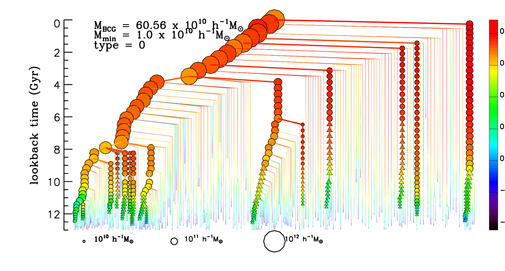
Figure 1: BCG merger tree. Symbols are colour–coded as a function of B - V colour and their area scales with the stellar mass. Only progenitors more massive than $10^{10}\,{\rm M}_{\odot}\,h^{-1}$ are shown with symbols. Circles are used for galaxies that reside in the FOF group inhabited by the main branch. Triangles show galaxies that have not yet joined this FOF group.

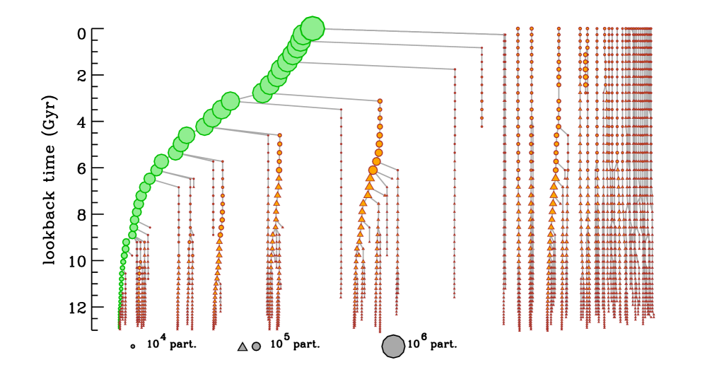
Figure 2: Merger tree of the FOF group in which the BCG sits at redshift zero. Only the trees of subhalos with more than $500$ particles at $z=0$ are shown. Their progenitors are shown down to a 100 particle limit. Symbol coding is the same as in Fig. 1. The left-most tree is that of the main subhalo of the FOF, while the trees on the right correspond to other substructures identified in the FOF group at $z=0$. In green, we mark the subhalo that contains the main branch of the BCG.

Fig. 1 shows the full merger tree of the central galaxy of a dark matter halo of mass ${\rm M}_{200}=8.9\times 10^{14}\,{\rm M}_{\odot}$ at $z=0$. The BCG itself lies at the top of the plot (at $z=0$), and all its progenitors (and their histories) are plotted downwards going back in time recursively. Galaxies with stellar mass larger (resp. smaller) than $10^{10}$ $h^{-1}$M_⊙ are shown as symbols (resp. lines), and are colour-coded as a function of their rest-frame B - V colour. The left-most branch in Fig. 1 represents what we will hereafter refer to as the main branch. This particular branch is obtained by connecting the galaxy at each time-step to the progenitor with the largest stellar mass (the main progenitor) at the immediately preceding time-step. It is tempting to consider this branch as the BCG itself, and the objects that merge onto it as other progenitors of the BCG. A clear distinction between “main” and “other” progenitors is indeed often quite appropriate - typically for late type galaxies - and it is satisfactory as long as galaxies merging onto the main branch have stellar masses that are much smaller than the current mass of the main progenitor. In this case, the evolution of the BCG can be characterised by a series of accretion events (of much smaller objects) that do not introduce major changes in the stellar population or identity of the BCG itself.

This simple summary of a merger tree is however not sufficient to describe histories as complex as those of BCGs (see also Neistein et al., 2006). Fig. 1 shows that in our case-study, the main branch captures the evolution of the BCG itself for the last $\sim 8$ Gyr. Before that time, the main progenitor of the BCG is only marginally more massive than progenitors in other branches. At this point, choosing one branch or another becomes arbitrary and a single branch is certainly a poor proxy for describing the evolution of the BCG and of its stellar population. In the following, we will simply refer to the main progenitor of the BCG at any given time as the main branch without implying that it necessarily contains most of the stars.

Galaxies that merge onto the main branch must first be accreted onto the same halo, and it is therefore interesting to establish the connection between the galaxy and the halo merger trees. Fig. 2 shows the full tree of the FOF-group containing our case-study BCG. The branch highlighted in green is the branch containing the main branch of the BCG. The right-most branches are merger trees of secondary substructures (only those with more than 500 particles) present in the FOF-group. These substructures have not yet dissolved into the main halo, and their galaxies can thus not contribute to the merger tree of the BCG. In Figs. 1 and 2 circles mark objects (galaxies or haloes) that belong to the same FOF group as the main branch of the BCG, while triangles mark objects that have not yet joined the FOF group. Typically, when a halo is accreted onto a bigger system (i.e. joins the same FOF group), it loses mass efficiently due to tidal stripping (Ghigna et al., 2000; Kravtsov et al., 2004; De Lucia et al., 2004; Gao et al., 2004). A nice example of this process is shown by the halo branch located roughly at the centre of Fig. 2. It is only when the subhalo dissolves that its galaxies become part of the main halo of the FOF group and are then allowed to merge with the central galaxy on a dynamical friction timescale.

Given the complexity of the merger history shown in Fig. 1, it is helpful to define several times that mark important phases in the evolution of a BCG. We call identity time ($t_{\rm{id}}$) the cosmic time when the BCG acquires its final identity. We define $t_{\rm{id}}$ as the time when the last major merger on the main branch occured, i.e. when the most massive galaxy which merges on the main branch is more massive than a third of the mass of the main progenitor. Before $t_{\rm{id}}$, the BCG does not exist as one single object, but as several progenitors of comparable masses. Our definition of the identity time can be extended to account for multiple simultaneous mergers. We thus define the extended identity time ($\tilde{t}_{\rm{id}}$) as the latest (cosmic) time when the sum of the masses of the progenitors merging on the main branch was larger than a third of the mass of the main progenitor. By definition, $t_{\rm{id}}\leq\tilde{t}_{\rm{id}}$, although they are equal in most cases (see Fig. 6 in Sec. 5).

Early theoretical work discussed the difference between formation and assembly times for elliptical galaxies in a hierarchical context (Baugh, Cole & Frenk, 1996; Kauffmann, 1996), although this difference has been quantified only recently (De Lucia et al., 2006). Following this work, we call assembly time ($t_{a}$) the time when the main progenitor contains half the final stellar mass of the BCG. As discussed above, although the main branch may capture the identity of a galaxy for some time, it is not suited to describe the complete evolution of the BCG. The stellar population of the BCG, in particular, can be fully described only by taking into consideration the whole tree, because a large fraction of stars actually form in secondary branches. It is therefore useful to define a more classical formation time ($t_{f}$) as the time when the total mass of stars formed reaches half the final mass of the BCG. By “total mass” we mean, at each cosmic time, the sum of the stellar masses of all the progenitors present at that given time, i.e. the projection of Fig. 1 onto the vertical time axis.

4.2 Mass build-up of the BCG

Fig. 1 shows that the stars that end up in the BCG today, start forming at very high redshifts. Rapid cooling in the early phases of the cluster collapse lead to the formation of a massive central galaxy of stellar mass $\sim 10^{11}\,{\rm M}_{\sun}\,h^{-1}$ about $11$ Gyr ago ($z\sim 2.5$). A number of accretions of massive satellites increases its mass to slightly less than half its present value at redshift about $1$ and then the BCG continues growing by accretion of satellites. Fig. 1 also clearly shows that the satellites accreted below redshift $\sim 1$ are red and much less massive than the main branch.

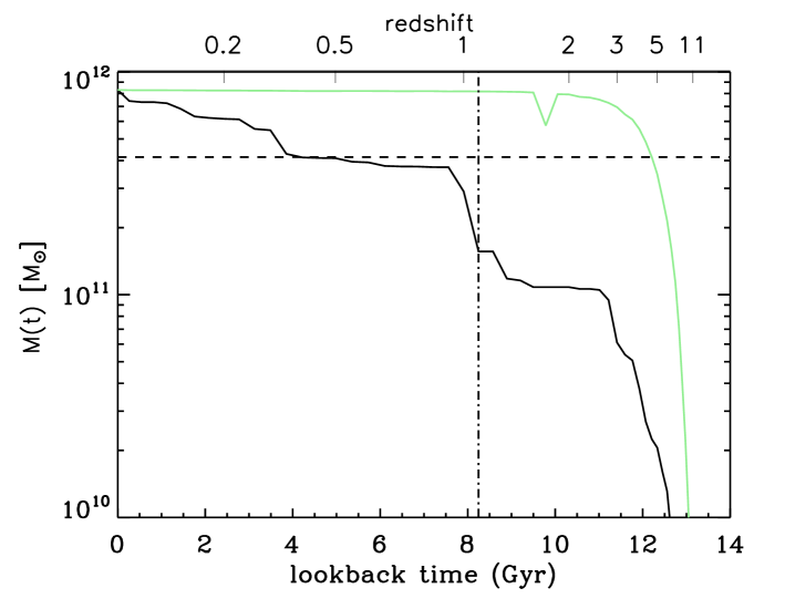
Figure 3: Formation and assembly histories of our case-study BCG. The black (resp. green) line shows the stellar mass in the main branch (resp. the mass summed over all progenitors) of our case-study BCG versus time. The horizontal dashed line corresponds to half the present mass of the BCG. The vertical lines mark the identity and extended identity times (see text for details).

In Fig. 3 we show the ‘formation’ and ‘assembly’ histories of the stars that end up in the BCG of our case-study cluster. The black line in Fig. 3 shows the stellar mass of the main branch. The green line shows the sum of the stellar masses in all progenitors at each time. The horizontal dashed line corresponds to half the present mass of the BCG. This figure clearly shows that while the main progenitor reaches half its final mass only at redshift $z_{a}\sim 0.5$, half of the stars are already formed at redshift $z_{f}\sim 5$. The identity time and the extended identity time are equal in this particular case and are indicated by the vertical line at $z\sim 1.2$.

It is now interesting to investigate in more detail how the BCG gained its mass and how the stars that end up in it were formed in the first place. Was star formation mainly triggered by starbursts in an early and dense environment? Or was star formation mostly quiescent, fuelled by rapid cooling?

Figure 4: Accretion history of our case-study BCG : fraction of the stellar mass that was brought by mergers onto the main branch. The solid line is the mass of the main branch. The 3-dot-dashed (resp. dot-dashed, dashed) line is the mass accreted by all (resp. more massive than $10^{10}$ $h^{-1}$M_⊙, less massive than $10^{10}$ $h^{-1}$M_⊙) galaxies merging on the main branch.

Fig. 4 shows the mass in the main branch as a function of time (solid line), and the fraction of it that was gained through accretion of galaxies (dash-3-dot curve). The dashed (resp. dot-dashed) curve indicates the contribution to accretion by galaxies with stellar masses lower (resp. larger) than $10^{10}$ $h^{-1}$M_⊙ (the same cut as in Fig. 1). Fig. 4 shows that most of the stars of this BCG were actually not formed in the main branch, but were instead accreted steadily over time. It is also interesting to note that, although the BCG tree has many branches, only a small fraction of these contribute significantly to the build-up of its mass: $\sim 70$ per cent of the mass comes from accretion of $12$ galaxies more massive than $10^{10}$ $h^{-1}$M_⊙. Note also that the main progenitor becomes rapidly massive enough that most galaxies falling onto the main branch give rise only to minor merger events. Fig. 4 shows that since $z\sim 4$ the mass growth of the main branch is only due to accretion: AGN activity has switched off cooling and hence star formation in the main branch. The stars that compose the BCG today formed in separate entities, mostly as a result of quiescent star formation: less than $10$ per cent of the stars were formed during starbursts (in agreement with previous results by Aragón-Salamanca et al., 1998). Note that this quiescent-to-bursty star formation ratio depends on the star formation prescription that we use for discs. The results of Somerville et al. (2001) and Baugh et al. (2005) suggest that our model predicts an upper boundary of this ratio.

In a hierarchical framework, the formation of a BCG naturally relates to the formation of the cluster itself. Fig. 5 shows how the stellar mass in the main branch (in orange) compares to the evolution of the dark matter (solid black line) and stellar content (dashed black line) of the halo in which the main progenitor of the BCG resides at each time. The red lines show instead the evolution in dark matter (solid) and stellar content (dashed) of all progenitors of the halo in which the galaxy sits today. Dark matter masses are normalised to the dark matter mass of the FOF group at redshift zero, while stellar masses are normalised to the total stellar content of the FOF group at redshift zero. The figure shows that the assembly history of the BCG follows the evolution of the dark matter and stellar content of its own halo with a delay due to dynamical friction. The parent halo of the BCG represents only $90$ per cent of the total mass of its parent FOF group, and its total stellar content accounts for about $35$ per cent of the stellar content of the FOF group. Note that although dark matter substructures only represent $\sim 10$ per cent of the mass of the FOF group, they contain about $65$ per cent of its stellar content. Interestingly, the total stellar content of all the progenitors of the halo increases very rapidly and stays constant after redshift $\sim 1$. This indicates that many substructures accreted below redshift $\sim 1$ survive as independent entities to the present day so that their galaxies do not contribute to the stellar content of the halo.

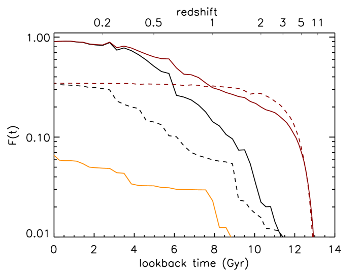
Figure 5: Evolution of the stellar content (dashed lines) and dark matter content (solid lines) of the subhalo in which our case-study BCG sits at $z=0$. Black and red lines are obtained by following the main progenitor only and all progenitors at any given redshift respectively. Dark matter masses are normalised to the dark matter mass of the FOF group at redshift zero, while stellar masses are normalised to the total stellar content of the FOF group at redshift zero. The orange line shows the stellar mass in the main branch.

5 Statistical results

In the previous section we have analysed in detail the formation and assembly history of one BCG chosen as a case study, and we have related these histories to the history of the parent halo itself. In this section, we extend this analysis to a statistical sample of BCGs selected from our simulation and study the dispersion in the quantities defined above. This is of particular interest because observed BCGs exhibit a remarkably small dispersion in their luminosities (see Sec. 1) and stellar population at low redshift (e.g. McNamara & O’Connell, 1989; James & Mobasher, 2000). This is commonly interpreted as a clear indication that these objects had similar formation histories. In order to address this point, we have selected the 125 haloes more massive than $7\times 10^{14}$ M_⊙ at $z=0$ from the Millennium Simulation and analysed their formation and assembly histories, as in the previous section. The BCGs of these objects have mean absolute magnitude ${\rm M}_{\rm K}=-26.58$ and a dispersion of $0.20$ mag. These values appear to be in nice agreement with observational results (see for example Fig. 10 in Collins & Mann, 1998). This agreement represents a major success of the underlying galaxy formation model.

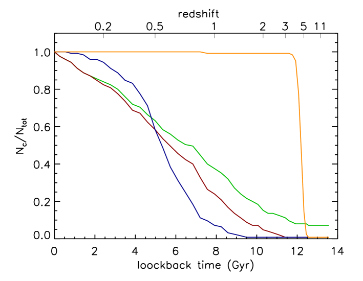
Figure 6: Fraction of clusters with identity (green), extended identity (red), assembly (blue) and formation (orange) lookback times larger than that shown on the x-axis.

In Fig. 6 we show the fraction of clusters with identity (green), extended identity (red), assembly (blue), and formation (orange) lookback times larger than that shown on the x-axis. The green line in Fig. 6 shows that for only about $40$ per cent of our BCGs was the last major merger before redshift $1$, and for $\sim 65$ per cent of them it occurred before redshift $\sim 0.5$. The numbers are slightly lower if one considers, instead of the time corresponding to the last major merger, the time when the sum of the masses of the accreted objects is equal to one third the mass in the main branch at the time of accretion (the extended identity time). The identity of the main progenitor of a redshift zero BCG is thus typically ill-defined before $z\sim 0.7$. The assembly times measured for our BCGs are low : half of them assembled after $z\sim 0.5$, and only 10 per cent of our BCGs assembled before $z\sim 1$. In contrast, for almost $100$ per cent of our BCGs, half of the stars were already formed at redshift larger than $4$, which indicates that all our BCGs have uniformly old stellar populations.

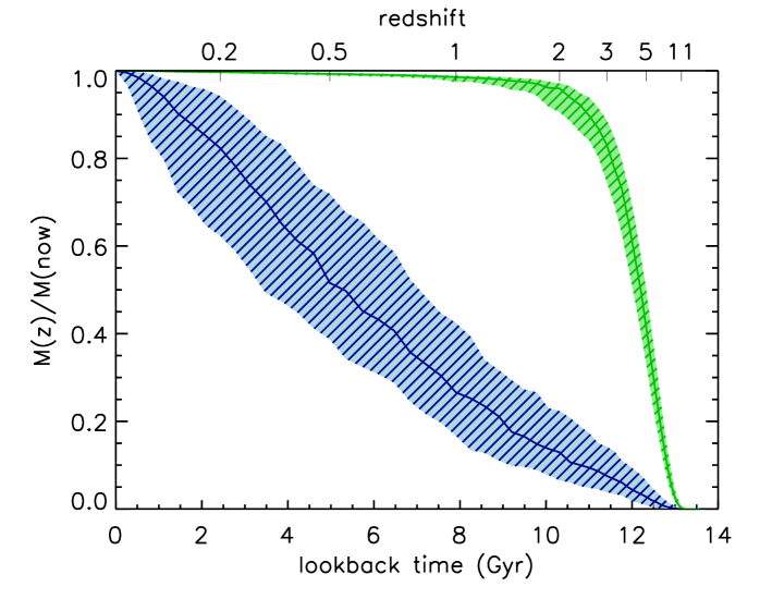
Figure 7: Assembly (blue) and formation (green) histories of our sample of BCGs selected at redshift $0$ (as in Fig. 3). Thick lines show the median of the distributions, while the dashed regions show the $15$th to $85$th percentile range.

Thick lines in Fig. 7 show the median assembly (blue) and formation (green) histories of our sample of redshift zero BCGs (as in Fig. 3). The dashed regions in this figure indicate the $15$th and $85$th percentiles of the distributions. Interestingly, there is a very small scatter in the formation histories of the BCGs: for essentially all the objects in our sample, $50$ per cent of the stars are already formed at redshift $5$ (as noticed from Fig. 6). The assembly histories exhibit a much larger scatter with the fraction of mass in the main progenitor varying between $15$ and $40$ per cent at redshift $1$, and between $40$ and $70$ per cent at redshift $0.5$. In Sec. 4, we have seen that the mass of the BCG mainly increases through accretion of satellites, Fig. 7 shows that this is the case for the whole sample. The difference between formation time and assembly time that we find here is higher than that found by De Lucia et al. (2006) for ellipticals, as expected from the “extreme” nature of BCGs. We note also that the we find a median mass growth of a factor $\sim 3$ from $z\sim 1$ to $z=0$. This is in apparent contradiction with observational data mentioned in Sec. 1. We will show that this is probably only an ‘apparent’ contradiction in Sec. 6.1.

Figure 8: Evolution of the dark matter mass of the FOF group containing the main progenitor of the BCG at each time (blue), of the stellar content of this FOF group (green), and of the mass of the main progenitor of the BCG (orange). Thick lines show the median and shaded regions show the $15$th to $85$th percentile range. Note that we have multiplied the stellar mass of the FOF group by a factor of $50$ and the mass of the main progenitor of the BCG by a factor of $100$.

Fig. 8 shows how the evolution of the mass in the main progenitor (orange) compares to the evolution in the stellar (green) and dark matter (blue) content of the FOF group in which the main progenitor resides at each lookback time. Thick lines show the median and shaded regions show the $15$th and the $85$th percentiles of the distributions. Note that we have multiplied the stellar mass of the FOF group by a factor of $50$ and the mass of the main progenitor of the BCG by a factor $100$ for display purposes. The figure shows that the stellar content of the FOF group in which the BCG sits, represents about $1.7$ per cent of its dark matter mass, at all redshifts. In turn, the mass in the main branch is $\sim 100$ per cent of the stellar content of the FOF group at high $z$, and then decreases to reach a plateau at $z\sim 1$, with a mass fraction of $\sim 6$ per cent.

The example in Fig. 1 shows that most of the progenitors accreted onto the main branch, are already red at the time of accretion. We now want to quantify the distribution of the objects accreted onto the main branch in terms of different physical properties. In Fig. 9 we show the distribution of these progenitors as a function of their gas fraction (panel a), star formation rate (panel b), stellar metallicity (panel c), and B - V colour (panel d). Note that we are using here only progenitors more massive than $10^{10}$ $h^{-1}$M_⊙, as these are the ones that contribute most significantly to the mass build-up of the BCG (see Fig. 4). The green histograms in all panels refer to all the objects accreted, independently of their accretion redshifts. The top left panel indicates that the great majority of these progenitors have very low gas fractions. Only objects accreted at very high redshift have some residual gas, as indicated by the red histograms; these refer to progenitors accreted at redshift larger than $3$. As a consequence, only objects accreted at very high redshift have some residual star formation (panel b) and relatively blue colours (panel d). Interestingly, the metallicity distribution of progenitors does not show any significant evolution with redshift. It peaks at $Z\sim 0.5Z_{\sun}$ and is quite broad.

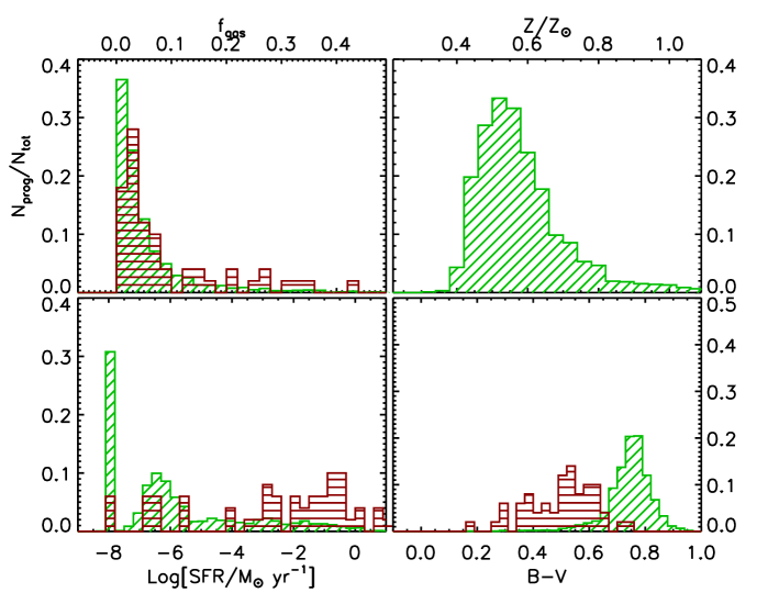
Figure 9: Distribution of objects accreted onto the main branch as a function of their gas fraction (panel a), star formation rate (panel b), stellar metallicity (panel c), and B - V colour (panel d). Green histograms refer to all progenitors, independently of their accretion redshifts. Red histograms refer to objects accreted at redshift larger than $3$.

Fig. 10 shows the morphological mix of the objects accreted onto the main branch in different redshift bins. We have determined the morphology of our model galaxies by using the B-band bulge-to-disc ratio together with the observational relation by Simien & de Vaucouleurs (1986) between this quantity and the galaxy morphological type. For the purposes of this analysis, we classify as early types all galaxies with $\Delta M<0.4$ ($\Delta M=M_{\rm bulge}-M_{\rm total}$), as late types all galaxies with $\Delta M>1.56$, and as lenticulars (S0) all galaxies with intermediate value of $\Delta M$. In Fig. 10, the red indicates early-type morphologies, the green is for S0 and the blue is for late types. For each redshift bin, the left-most histogram refers to normalisation by mass, while the right-most histogram refers to normalisation by the number of objects. The number of objects accreted in each redshift bin is indicated on the top of the histograms. The figure clearly shows that, with the exception of the highest redshift bin considered, the majority of the objects accreted onto the main branch, already have an early-type morphology.

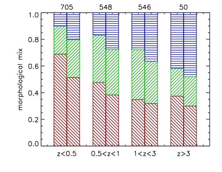
Figure 10: Morphological mix of objects accreted onto the main branch in different redshift bins. The red indicates early-type morphologies, the green is for S0 and the blue is for late types (see text for details). For each redshift bin, the left-most histogram refers to a normalisation in mass, while the right-most histogram refers to a normalisation in number.

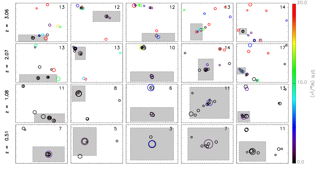
Figure 11: Spatial distribution of the progenitors of five model BCGs at redshifts $\sim$ 0.5, 1, 2 and 3. Progenitors more massive than $10^{10}h^{-1}M_{\odot}$ are shown using symbols colour-coded with star formation rate and with size scaling with stellar mass. The number in the upper-right corner of each panel indicates the number of such progenitors. The gray area marks a $2\times 2$ Mpc² comoving region centred on the main progenitor of the redshift zero BCG.

We saw previously that a BCG is not well described by the monolithic approximation. Instead, at $z>0$, a BCG breaks into an ensemble of distinct galaxies, and it is all of them at the same time. A question relevant both to the theoretical and observational sides is then: what is the spatial extent of the progenitor set as a function of time? In other words, how far do the progenitors of the BCG extend? Fig. 11 shows the spatial distribution of progenitors of five model BCGs at different redshifts. Only progenitors more massive than $10^{10}$ $h^{-1}$M_⊙ are shown, with symbols that scale with mass as in Fig. 1. The symbols are colour-coded by the star formation rate averaged over a time-step ($\sim 200$ Myr). The number of progenitors more massive than $10^{10}h^{-1}M_{\odot}$ is indicated in the upper-right corner of each panel. The gray area marks a $2\times 2$ Mpc² comoving region and is centred on the main progenitor of the BCG. The typical extent of the progenitors goes from $\sim 10h^{-1}$Mpc (comoving) at $z=3$ down to about $\sim 1h^{-1}$Mpc at $z=0.5$. Several panels (e.g. middle panels down to $z\sim 1$) show that the main progenitor of the BCG is not necessarily the most massive progenitor at that redshift.

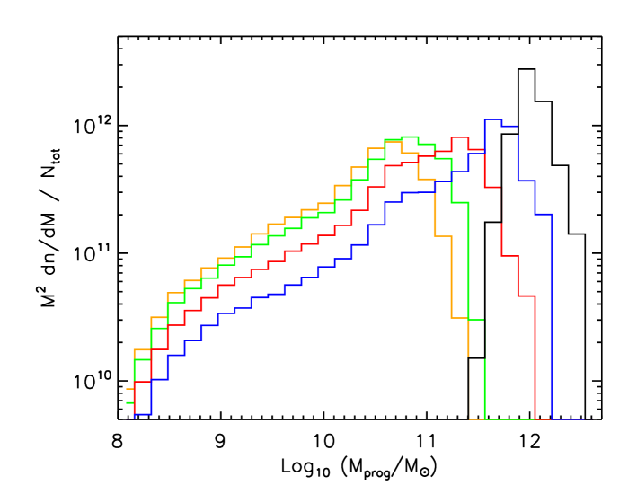
Figure 12: Stellar mass distribution for the progenitors of local BCGs at redshifts 0.5 (blue), 1 (red), 2 (green), and 3 (orange). The black histogram shows the stellar mass distribution of local BCGs.

Fig. 12 shows the stellar mass distribution of progenitors of redshift zero BCGs at redshifts 0.5 (blue), 1 (red), 2 (green), and 3 (orange). The black histogram shows the stellar mass distribution of local BCGs. The figure clearly shows that the mass distribution of progenitors of local BCGs becomes broader and more skewed towards lower masses with increasing redshift. At redshift $\sim 1$ the massive tail of the progenitors of local BCGs are about a factor $3$ smaller than redshift zero BCGs. This factor rises to about $10$ at $z\sim 3$.

6 The evolution of high-L_X BCGs

In the previous sections, we discussed one facet of the evolution of BCGs, namely: how did low redshift BCGs form? We now want to address this issue from an observational perspective. For example, we want to ask if the low assembly times measured for our local sample of BCGs are in agreement with observational results for high-L_X clusters. This raises two complementary questions:

• How do the properties of high-$z$ BCGs differ from those of local ones? In other words, what is the observable evolution of BCGs ?

• What is the hierarchical relationship (if any) between BCGs observed at different redshifts? In other words, are high-$z$ BCGs progenitors of low-$z$ BCGs and are low-$z$ BCGs descendants of high-$z$ BCGs?

We extend the sample used in the previous section by selecting the $125$ central galaxies lying in the most massive haloes at $6$ different redshifts : $z\sim\{0.2;0.5;0.75;1;1.5;2\}$. Our selection corresponds to a selection in mass with lower mass limits equal to $M_{h}/(10^{14}M_{\odot})=\{5.4;3.7;2.7;1.9;1.2;0.67\}$ respectively. We chose this somewhat arbitrary mass selection so as to preserve the same number density of BCGs at all redshifts. This choice would correspond to the (incorrect) monolithic assumption in which each local BCG has a well-defined dominant progenitor at each redshift. Given that we select the most massive haloes at each time-step, our sample is qualitatively comparable to selecting the highest luminosity X-ray clusters at each redshift down to a fixed comoving abundance.

6.1 Observable evolution

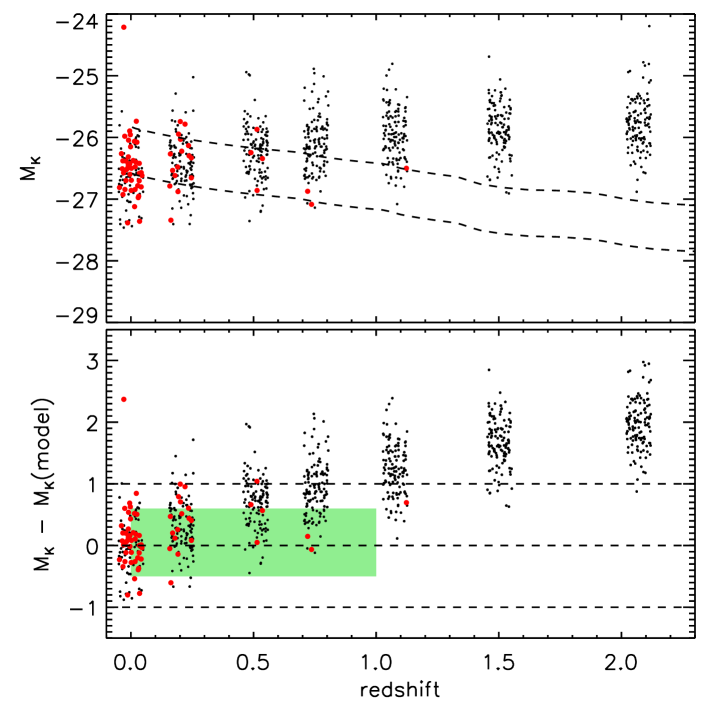
Figure 13: Evolution of the rest-frame $K$-band absolute magnitude of BCGs as a function of redshift. Black points show model BCGs (a small random spread has been added along the x-axis for clarity), and the red symbols refer to BCGs of haloes more massive than $10^{15}\,{\rm M}_{\odot}$. In the upper panel, the dashed lines shows predictions from a single burst model with redshift of formation $5$. The lower line is normalised to the median magnitude of local BCGs, and the upper one refers to a normalisation fainter by a factor $2$. In the lower panel, black points show the residuals with respect to the model with median normalisation. The shaded (green) area shows the rough location of observations (see text for details).

In the upper panel of Fig. 13, we show the rest-frame K-band absolute magnitude distribution of the (low- and) high-$z$ model BCGs. Each galaxy is represented with a small random offset with respect to its redshift, for clarity. The lower dashed line in this panel shows the magnitude decline predicted by a single burst model where all the stars are formed at $z=5$ and evolved passively to the present day. This line is normalised to the median magnitude of the local sample. The upper line refers to a normalisation fainter by a factor $2$. The model has been built using the Bruzual & Charlot (2003) code with a solar metallicity stellar population and a Salpeter IMF with lower and upper mass cutoffs $m_{l}=0.1\,{\rm M}_{\sun}$ and $m_{u}=100\,{\rm M}_{\sun}$. In the lower panel of Fig. 13, we show the residuals of the K-band magnitudes of our model BCGs with respect to the single burst model (median normalisation), as a function of redshift. In both panels, the red symbols highlight BCGs of haloes more massive than $10^{15}\,{\rm M}_{\odot}$. Using the local observational relation between ${\rm M}_{200}$ and L_X (Popesso et al., 2005), this mass cut roughly corresponds to the L${}_{\rm X}>2.3\times 10^{44}\,{\rm erg}\,{\rm s}^{-1}$ cut used by Burke et al. (2000).

As mentioned before, our low-$z$ BCGs cover the same range of absolute K-band magnitudes as measured for high-L_X clusters. Model data shown in the top panel of Fig. 13 indicate that the predicted mass growth between $z\sim 1$ and $z=0$ is of about a factor $3$. We note that this is the same factor measured in Fig. 7 following the main branch of local BCGs. This appears as a coincidence since high-$z$ BCGs are a priori different from progenitors of local BCGs (see next subsection). This predicted mass growth also seems to be in conflict with observational results. The latter are, however, based on high-L_X clusters, roughly more massive than $10^{15}\,{\rm M}_{\odot}$. Red symbols in the top panel of Fig. 13 show that selecting haloes above a fixed mass cut corresponds to selection of “rarer” systems at higher redshifts. For model BCGs sitting in these haloes, the mass growth is less than a factor $2$ between $z=1$ and $z=0$. Although based on low-number statistics, this result is compatible with that inferred from observational data.

In the bottom panel of Fig. 13, we reproduce the analysis by Burke et al. (2000). The shaded (green) area in this panel marks the rough location of their results. The red symbols again show that a selection above a fixed mass cut gives a good agreement with these observational data. The evolution of ‘rarest’ BCGs also appears to be in agreement with passive evolution. We find, however, that this does not hold if the selection is extended to lower mass systems.

The above comparisons should be considered only as a qualitative indication. Burke et al. (2000) use observed aperture magnitudes (measured adopting a $50\,{\rm kpc}$ diameter aperture) and make no attempt to remove the flux due to other galaxies falling within the aperture. They also use a different model normalisation along with a number of different details.

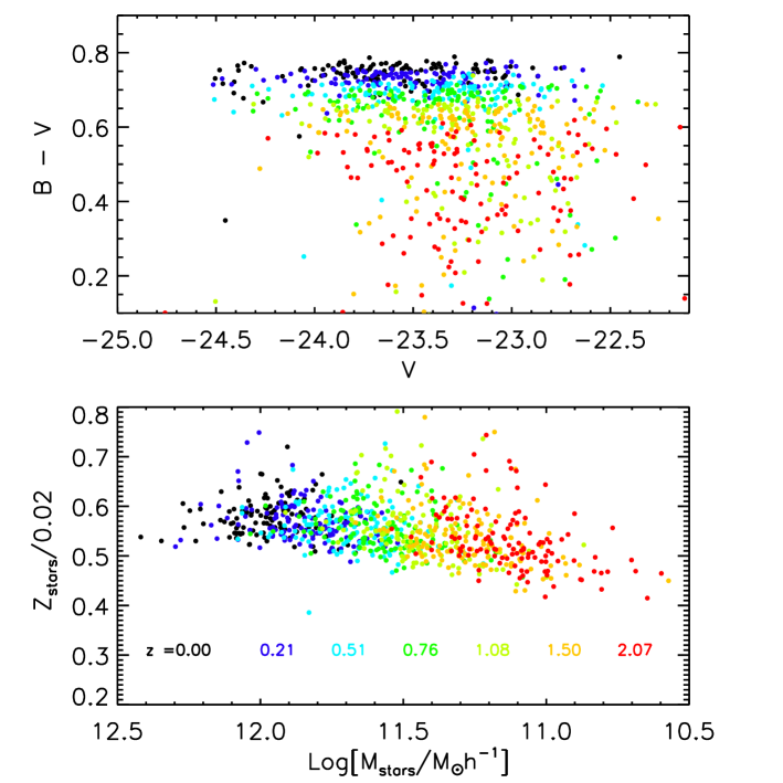
Figure 14: Upper panel : colour-magnitude relation for BCGs as a function of redshift. Symbols are colour-coded with increasing redshift from black to red. Lower panel : mass-metallicity relation, and its evolution as a function of redshift.

In Fig. 14 we show the rest-frame colour–magnitude (AB) relation (upper panel) and the relation between the stellar mass and metallicity (lower panel) for our model BCGs. Symbols are colour–coded with increasing redshift from black to red. The amount of reddening we measure between redshift $\sim 2$ and redshift $0$ is $\sim 0.2$ (considering the median colour for each redshift bin), which is very close to the amount predicted by the single burst model used above. Interestingly the colour–magnitude relation for our model BCGs has very little slope at any redshift. The mass–metallicity relation shown in the bottom panel of Fig. 14 exhibits a more significant, although still weak, slope.

The results presented in this section change if a different supernovae feedback model is used. Our default model in this paper is the supernova feedback model used in Croton et al. (2006), in which the ejection rate is proportional to the star formation rate. We have repeated our analysis using the supernova feedback model of De Lucia et al. (2006), where the ejection rates are computed on the basis of energy conservation arguments. This model results in less efficient winds in massive galaxies and, as a consequence in more prolonged star formation activity. While this does not significantly change results presented in previous sections, it results in slower evolution of the K-band magnitudes as a function of redshift which brings more model points into agreement with the observational data. However, the K-band magnitudes of local BCGs are then predicted to be about $0.8$ mag brighter and are typically more luminous than observed systems. This different feedback scheme also produces a larger scatter in the colours and metallicities of model BCGs at all redshifts, as well as stellar metallicities that are larger than those shown in Fig. 14 by a factor of $\sim 2$. The former is a consequence of the more extended star formation activity, the latter of the processing of larger amounts of gas into stars.

6.2 Hierarchical evolution

In a hierarchical scenario, high-$z$ BCGs are not necessarily the progenitors of local ones. In this section we want to assess the overlap between these two populations.

A first question is: what is the fraction of high-$z$ BCGs which do not end-up in our local sample? In Fig. 15, we show this fraction as a function of redshift. We have highlighted in red (resp. blue) the contribution of BCGs residing in haloes less (resp. more) massive than the median mass of our samples at each redshift, as indicated on the plot. A striking remark from Fig. 15 is that $\sim 70$ per cent of our BCGs at $z=2$ do not become part of local BCGs, and this does not appear to depend strongly on the mass of their host haloes. However, this fraction of “lost” BCGs decreases with redshift, as expected, and does so more rapidly for BCGs sitting in more massive haloes. We note that high-$z$ BCGs, although they do not necessarily end up in our local BCGs, do end up in massive galaxies at the centre of massive haloes at $z=0$. This is illustrated in Fig. 16, which shows the mass of haloes harbouring high-$z$ BCGs versus the mass of the haloes harbouring their descendants at $z=0$. In this figure, open triangles indicate “lost” BCGs, whereas open circles indicate BCGs that end-up in our local sample. This figure shows that descendents of high-$z$ BCGs simply extend towards lower masses our local sample of clusters and we emphasise that this does not suggest that “lost” BCGs are in any way a different population.

Turning the question around, we can assess whether the massive progenitors of our local sample are different from high-$z$ BCGs. Fig. 17 shows the stellar mass distribution of high-$z$ BCGs (red histograms), and that of the progenitors of our local BCGs (blue histograms). These distributions are both normalised to the number of BCGs at each redshift (i.e. 125). Overlap of the histograms does not imply that they include the same galaxies, but just that objects of given mass have equal number densities. At redshift lower than $\sim 0.7$, model BCGs are ‘assembled’ (see Fig. 6), and indeed, the main branch stands out at the massive end of the blue histograms. There is then a rather good overlap between the mass distributions of high-$z$ BCGs and the massive progenitors of local BCGs. Moving to higher redshift, the massive tail of progenitors disappears. As we showed, this is because typically at $z\mathchar 13350\relax 0.7$ no branch has yet become dominant in the trees of local BCGs. At these redshifts, high-$z$ BCGs still have a similar mass distribution as the massive progenitors of local BCGs, although Fig. 15 shows they are not the same objects.

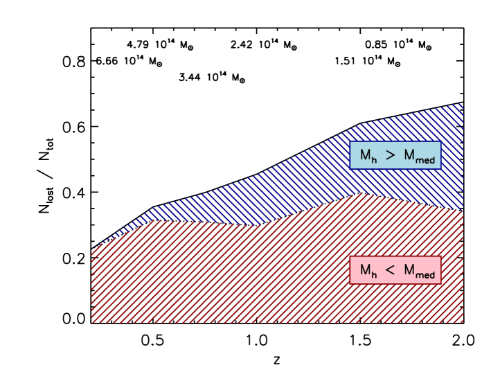
Figure 15: Fraction of high-$z$ BCGs that do not end up in our sample of local BCGs. The red area shows contribution from BCGs residing in haloes with mass lower than the median mass measured for the sample at each of the redshifts considered. The blue area shows the contribution from massive haloes.

At first sight, it may be surprising that our high-$z$ BCGs do not end up in our local sample. However, we showed that they do belong to the same population as progenitors of local BCGs, and do end up as central galaxies of massive haloes. The evolution seen in Fig. 15 then appears to be essentially driven by the evolution of dark matter haloes. The most massive haloes at $z=2$ are not in general the progenitors of the most massive haloes at $z=0$ and therefore the BCGs they contain just fall out of our local sample.

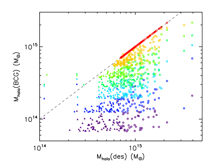
Figure 16: Halo mass distributions. The y-axis shows the masses of haloes hosting BCGs at the redshift they are observed; the x-axis shows the masses of haloes containing their descendants at $z=0$. Triangles indicate “lost” BCGs and open circles indicate BCGs that end-up in local BCGs. The colour-coding indicates redshift, decreasing from purple to red.

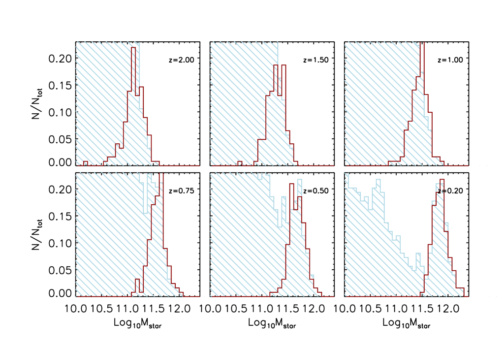
Figure 17: Stellar-mass distribution of high-$z$ BCGs (red histograms) and of progenitors of local BCGs (blue histograms). Both histograms are normalised to the total number of BCGs at each redshift (125).

7 Conclusions and discussion

In this study, we have used a combination of high-resolution $N$-body simulations and semi-analytic techniques to investigate the formation and evolution of BCGs in a cosmological context. This allows us to explicitly take into account the full hierarchy of dark matter structure growth, and its impact on galaxy formation. We show that in a CDM Universe, this hierarchical build-up implies that central galaxies of massive haloes have complex merging histories that are not well described by monolithic approximations.

In the first part of our paper, we have studied in detail the formation and assembly histories of local BCGs. We find that the stars in these systems start forming very early (about $50$ per cent of the stars in these systems have already formed by redshift $\sim 5$) although the identity of the BCGs themselves is not defined before $z\sim 0.7$. A monolithic approximation clearly fails to describe these objects for most of their history. Most of the stars are formed in separate entities in a quiescent mode and most of the mass in the local BCGs is gained through accretion of a relatively low number (typically $10$) of objects more massive than $10^{10}\,h^{-1}{\rm M}_{\odot}$. Most of these accreted objects, with the exception of those accreted at very high redshift, have very low gas fractions and star formation rates, quite red colours and an early-type morphology. Interestingly, the main branches of BCGs grow fast enough that very few major mergers occur along them, most of the accretion events being minor mergers.

It is worth mentioning that our quantitative results do depend strongly on the implemented feedback models, both from AGNs and from supernovae. The AGN feedback model employed here (Croton et al., 2006) is extremely efficient in switching off cooling in relatively massive haloes even at high redshifts. At the same time, the supernova feedback model we use (also from Croton et al., 2006) drives strong winds that blow out all the gas from galaxies on short timescales. The combination of these two processes causes the early shutdown of star formation in the progenitors of local BCGs. These two particular feedback implementations are among the most efficient proposed so far in the literature. The work presented here leaves room for less drastic alternatives.

In the second part of our work, we have studied the observable evolution of BCGs by selecting the $125$ most massive haloes at different redshifts. From these samples of high-$z$ BCGs, we measure a mass growth of a factor of $\sim 3$ from $z=1$ to $z=0$. This is by coincidence very close to the growth we find following the main branch of local BCGs. These mass growth factors are higher than those inferred from observational data. However, when we use a selection that more closely matches that of high-L_X clusters, we find milder evolution, consistent with the observations. Interestingly we find that our model BCGs exhibit, at all redshifts, a weak correlation between stellar mass and stellar metallicity and an even weaker correlation between their magnitudes and their colours. This changes slightly if a different supernova feedback model is employed. Our high-$z$ BCGs do end up as central galaxies of massive haloes at $z=0$ but, because of our cluster sample selection criterion, many of their descendants are not included in our local BCG sample. However, we have shown that there is no substantive physical difference (1) between local BCGs and the descendents of high-$z$ BCGs, and (2) between high-$z$ BCGs and the most massive progenitors of local BCGs.

References

- Aragón-Salamanca et al. (1998) Aragón-Salamanca A., Baugh C. M., Kauffmann G., 1998, MNRAS, 297, 427
- Baugh et al. (1996) Baugh C. M., Cole S., Frenk C. S., 1996, MNRAS, 283, 1361
- Baugh et al. (2005) Baugh C. M., Lacey C. G., Frenk C. S., Granato G. L., Silva L., Bressan A., Benson A. J., Cole S., 2005, MNRAS, 356, 1191
- Bernstein & Bhavsar (2001) Bernstein J. P., Bhavsar S. P., 2001, MNRAS, 322, 625
- Binney & Tremaine (1987) Binney J., Tremaine S., 1987, Galactic dynamics. Princeton, NJ, Princeton University Press, 1987, 747 p.
- Brough et al. (2002) Brough S., Collins C. A., Burke D. J., Mann R. G., Lynam P. D., 2002, MNRAS, 329, L53+
- Bruzual & Charlot (2003) Bruzual G., Charlot S., 2003, MNRAS, 344, 1000
- Burke et al. (2000) Burke D. J., Collins C. A., Mann R. G., 2000, ApJ, 532, L105
- Chabrier (2003) Chabrier G., 2003, PASP, 115, 763
- Charlot & Fall (2000) Charlot S., Fall S. M., 2000, ApJ, 539, 718
- Collins & Mann (1998) Collins C. A., Mann R. G., 1998, MNRAS, 297, 128
- Cox et al. (2004) Cox T. J., Primack J., Jonsson P., Somerville R. S., 2004, ApJ, 607, L87
- Cowie & Binney (1977) Cowie L. L., Binney J., 1977, ApJ, 215, 723
- Croton et al. (2006) Croton D. J., Springel V., White S. D. M., De Lucia G., Frenk C. S., Gao L., Jenkins A., Kauffmann G., Navarro J. F., Yoshida N., 2006, MNRAS, 365, 11
- De Lucia et al. (2004) De Lucia G., Kauffmann G., Springel V., White S. D. M., Lanzoni B., Stoehr F., Tormen G., Yoshida N., 2004, MNRAS, 348, 333
- De Lucia et al. (2004) De Lucia G., Kauffmann G., White S. D. M., 2004, MNRAS, 349, 1101
- De Lucia et al. (2006) De Lucia G., Springel V., White S. D. M., Croton D., Kauffmann G., 2006, MNRAS, 366, 499
- Devriendt et al. (1999) Devriendt J. E. G., Guiderdoni B., Sadat R., 1999, A&A, 350, 381
- Dressler (1978) Dressler A., 1978, ApJ, 223, 765
- Dubinski (1998) Dubinski J., 1998, ApJ, 502, 141
- Fabian (1994) Fabian A. C., 1994, ARA&A, 32, 277
- Gao et al. (2004) Gao L., Loeb A., Peebles P. J. E., White S. D. M., Jenkins A., 2004, ApJ, 614, 17
- Gao et al. (2004) Gao L., White S. D. M., Jenkins A., Stoehr F., Springel V., 2004, MNRAS, 355, 819
- Ghigna et al. (2000) Ghigna S., Moore B., Governato F., Lake G., Quinn T., Stadel J., 2000, ApJ, 544, 616
- Guiderdoni & Rocca-Volmerange (1987) Guiderdoni B., Rocca-Volmerange B., 1987, A&A, 186, 1
- Gunn & Oke (1975) Gunn J. E., Oke J. B., 1975, ApJ, 195, 255
- Hatton et al. (2003) Hatton S., Devriendt J. E. G., Ninin S., Bouchet F. R., Guiderdoni B., Vibert D., 2003, MNRAS, 343, 75
- Hoessel & Schneider (1985) Hoessel J. G., Schneider D. P., 1985, AJ, 90, 1648
- James & Mobasher (2000) James P. A., Mobasher B., 2000, MNRAS, 317, 259
- Jones & Forman (1984) Jones C., Forman W., 1984, ApJ, 276, 38
- Kauffmann (1996) Kauffmann G., 1996, MNRAS, 281, 487
- Kauffmann & Haehnelt (2000) Kauffmann G., Haehnelt M., 2000, MNRAS, 311, 576
- Kong et al. (2004) Kong X., Charlot S., Brinchmann J., Fall S. M., 2004, MNRAS, 349, 769
- Kravtsov et al. (2004) Kravtsov A. V., Gnedin O. Y., Klypin A. A., 2004, ApJ, 609, 482
- Kroupa (2001) Kroupa P., 2001, MNRAS, 322, 231
- Lemson & the Virgo Consortium (2006) Lemson G., the Virgo Consortium 2006, astro-ph/0608019
- Malumuth & Richstone (1984) Malumuth E. M., Richstone D. O., 1984, ApJ, 276, 413
- Mathis et al. (1983) Mathis J. S., Mezger P. G., Panagia N., 1983, A&A, 128, 212
- McNamara & O’Connell (1989) McNamara B. R., O’Connell R. W., 1989, AJ, 98, 2018
- Merritt (1985) Merritt D., 1985, ApJ, 289, 18
- Neistein et al. (2006) Neistein E., van den Bosch F. C., Dekel A., 2006, MNRAS, pp 1043–+
- Nipoti et al. (2003) Nipoti C., Stiavelli M., Ciotti L., Treu T., Rosati P., 2003, MNRAS, 344, 748
- Oemler (1976) Oemler Jr. A., 1976, ApJ, 209, 693
- Ostriker & Tremaine (1975) Ostriker J. P., Tremaine S. D., 1975, ApJ, 202, L113
- Popesso et al. (2005) Popesso P., Biviano A., Böhringer H., Romaniello M., Voges W., 2005, A&A, 433, 431
- Postman & Lauer (1995) Postman M., Lauer T. R., 1995, ApJ, 440, 28
- Quintana & Lawrie (1982) Quintana H., Lawrie D. G., 1982, AJ, 87, 1
- Rhee & Latour (1991) Rhee G. F. R. N., Latour H. J., 1991, A&A, 243, 38
- Sánchez et al. (2006) Sánchez A. G., Baugh C. M., Percival W. J., Peacock J. A., Padilla N. D., Cole S., Frenk C. S., Norberg P., 2006, MNRAS, 366, 189
- Sandage (1972) Sandage A., 1972, ApJ, 178, 1
- Schombert (1986) Schombert J. M., 1986, ApJS, 60, 603
- Silk (1976) Silk J., 1976, ApJ, 208, 646
- Simien & de Vaucouleurs (1986) Simien F., de Vaucouleurs G., 1986, ApJ, 302, 564
- Somerville et al. (2001) Somerville R. S., Primack J. R., Faber S. M., 2001, MNRAS, 320, 504
- Springel et al. (2005) Springel V., White S. D. M., Jenkins A., Frenk C. S., Yoshida N., Gao L., Navarro J., Thacker R., Croton D., Helly J., Peacock J. A., Cole S., Thomas P., Couchman H., Evrard A., Colberg J., Pearce F., 2005, Nature, 435, 629
- Springel et al. (2001) Springel V., White S. D. M., Tormen G., Kauffmann G., 2001, MNRAS, 328, 726
- Tremaine & Richstone (1977) Tremaine S. D., Richstone D. O., 1977, ApJ, 212, 311
- White (1976) White S. D. M., 1976, MNRAS, 174, 19
- Zabludoff et al. (1990) Zabludoff A. I., Huchra J. P., Geller M. J., 1990, ApJS, 74, 1