Anisotropic Galactic Outflows and Enrichment of the Intergalactic Medium. I: Monte Carlo Simulations

Abstract

We have developed an analytical model to describe the evolution of anisotropic galactic outflows. With it, we investigate the impact of varying opening angle on galaxy formation and the evolution of the intergalactic medium. We have implemented this model in a Monte Carlo algorithm to simulate galaxy formation and outflows in a cosmological context. Using this algorithm, we have simulated the evolution of a comoving volume of size $(12h^{-1}{\rm Mpc})^{3}$ in the $\Lambda$CDM universe. Starting from a Gaussian density field at redshift $z=24$, we follow the formation of $\sim 20,000$ galaxies and simulate the galactic outflows produced by these galaxies. When these outflows collide with density peaks, ram pressure stripping of the gas inside the peaks may result. This occurs in around half the cases and prevents the formation of galaxies. Anisotropic outflows follow the path of least resistance and thus travel preferentially into low-density regions, away from cosmological structures (filaments and pancakes) where galaxies form. As a result, the number of collisions is reduced, leading to the formation of a larger number of galaxies. Anisotropic outflows can significantly enrich low-density systems with metals. Conversely, the cross-pollution in metals of objects located in a common cosmological structure, like a filament, is significantly reduced. Highly anisotropic outflows can travel across cosmological voids and deposit metals in other, unrelated cosmological structures.

1 INTRODUCTION

Galactic outflows play an important role in the evolution of galaxies and the intergalactic medium (IGM). Supernova explosions in galaxies create galactic winds, which deposit energy and metal-enriched gas into the IGM. These outflows are necessary to explain many observations and to solve many problems in galaxy formation, such as the high mass-to-light ratio of dwarf galaxies, the observed metallicity of the IGM, the entropy content of the IGM, the abundance of dwarf galaxies in the Local Group, the overcooling problem, and the angular momentum problem.

High-resolution, gasdynamical simulations of explosions in a single object reveal that outflows generated by such explosions tend to be highly anisotropic, with the energy and metal-enriched gas being channeled along the direction of least resistance, where the pressure is the lowest (Mac Low & Ferrara, 1999; Martel & Shapiro, 2001a, b). Furthermore, several observations support the existence of anisotropic outflows (e.g. Bland & Tully 1988; Fabbiano, Heckman, & Keel 1990; Carignan et al. 1998; Shopbell & Bland-Hawthorn 1998; Strickland et al. 2000; Veilleux & Rupke 2002).

Indirect support for the existence of anisotropic outflows comes from the observed enrichment of systems around the mean density of the universe (Schaye et al., 2003; Pieri & Haehnelt, 2004) and the enrichment of systems far from known galaxies at $z\sim 3$ (Pieri, Schaye, & Aguirre, 2006; Songaila, 2006). It may be challenging to enrich such regions with isotropic outflows even with the inclusion of enrichment from poorly understood Population III stars. Early indications are that Population III stars are unlikely to pollute the IGM to a large extent (Norman, O’Shea, & Paschos, 2004). Anisotropic outflows may also provide an explanation for part of the observed scatter in the metallicity in the IGM, which is still unexplained (Schaye et al., 2003; Pieri, Schaye, & Aguirre, 2006).

Several simulations of galactic outflows in cosmological contexts have been performed. Typically, these simulations use cubic comoving volumes of size $\sim(10\,{\rm Mpc})^{3}$, containing thousands of galaxies. The methods used can be divided into two groups : analytical methods and numerical methods. The analytical methods describe the expansion of outflows in simulations that are either Gaussian random realizations of the density power spectrum or N-body simulations combined with prescriptions for galaxy formation. Outflows are represented using an analytical solution (e.g. Scannapieco & Broadhurst 2001, hereafter SB01, Theuns, Mo, & Schaye 2001; Bertone, Stoehr, & White 2005) that currently assume isotropy.

The numerical simulations use hydrodynamical algorithms such as SPH, and outflows are generated in a variety of ways: by imparting SPH particles with a large velocity component (e.g. Scannapieco, Thacker, & Davis 2001; Springel & Hernquist 2003; Oppenheimer & Davé 2006), depositing additional thermal energy into SPH particles (e.g. Theuns et al. 2002b), or taking output from completed SPH simulations and calculating, a posteriori, the propagation of outflows into the IGM (Aguirre et al., 2001). Unlike the analytical methods cited above, which assume isotropic outflows, all these numerical approaches have the potential to generate anisotropic outflows. However, we believe that there are some limitations to these numerical approaches, which motivates us to introduce an analytical model for anisotropic outflows.

With any SPH simulation, we need to be concerned with the limited resolution of the algorithm. Consider for example the simulations of Scannapieco, Thacker, & Davis (2001). These authors identify galaxies of radius $r_{N}$, and rearrange the SPH particles located between $r_{N}$ and $r_{0}=2r_{N}$ into two uniform, concentric spherical shells located at radii $0.9r_{0}$ and $r_{0}$, which are then given an outward velocity. The outflow is therefore initially isotropic but becomes anisotropic as it propagates into a non-uniform external medium. We can see two potential problems with this approach. Firstly, the structure responsible for generating the anisotropy might be the galaxy or its environment, in which case the rearranging of particles into concentric shells would erase that structure entirely. Secondly, 52 particles per shell (the number they used) provides a good covering of the solid angles initially, but as the outflow expands and the particles in the shells move apart they become more like individual pressure points pushing on the external medium, and this could lead to an artificial mixing of the outflow and the external medium by Raleigh-Taylor instability.

The approach of Aguirre et al. (2001) is radically different. It consists of identifying galaxies in an output from an SPH simulation and calculating the propagation of outflows from these galaxies in $N_{a}$ different directions. Since the resistance encountered by the outflows will be direction-dependent, outflows will start isotropic but then become anisotropic as the distance travelled by outflows will vary with direction. There are two limitations to this approach. Firstly, since it uses the output of an SPH simulation and introduces the outflows a posteriori, the feedback effect of these outflows cannot be simulated (i.e. outflows do not influence the formation of other galaxies). Secondly, in this approach gas elements move radially and encountering high-pressure gas will dissipate their energy and rapidly slow down. In the real universe, that gas element will likely acquire a tangential velocity component that will redirect it towards regions where the resistance of the external medium is weaker.

To overcome these various limitations and study anisotropic outflows in a cosmological context, including the effect of feedback, we have designed an analytical model for galactic outflows. This can then be combined with either an analytical method or a semi-analytic method for the description of galaxy formation. In this paper, we use an analytical Monte Carlo method. Calculations performed with an N-body semi-analytic approach will be presented in a forthcoming paper (Martel, Grenon, & Pieri, 2007).

This paper is set out as follows. In §2, we describe our analytical model for anisotropic outflows. In §3, we describe our Monte Carlo method for cosmological simulations. Results are presented in §4, and their implications are discussed in §5. Conclusions are presented in §6.

2 A MODEL FOR ANISOTROPIC OUTFLOWS

Consider a density field with a local density maximum at some position, $P$. A halo may collapse at that point and may go on to form a galaxy, which will then produce an outflow. Our goal is to design an analytical model for the geometry and evolution of this outflow that takes into account the physical properties of the galaxy, the density distribution of the matter surrounding the galaxy, and the global properties of the IGM.

Using the high-resolution simulations and the observations of galactic outflows as a guide, we will represent outflows as “bipolar spherical cones.” In a spherical coordinate system $(r,\theta,\phi)$, the outflow occupies the volume defined by $r\leq R(t)$, $\theta\leq\alpha/2$ or $\theta\geq\pi-\alpha/2$, and $0\leq\phi<2\pi$ where $R(t)$ is the radius of the outflow and $\alpha$ is the opening angle. This is illustrated in Figure 1.

Figure 1: Geometry of the isotropic and anisotropic outflows. The isotropic outflows are spherical; the anisotropic ones are bipolar spherical cones. $R(t)$ is the time-dependent radius of the outflow, $\alpha$ is the opening angle, and $\hat{\bf e}$ the direction of the outflow.

In the limit $\alpha=\pi$, the outflow becomes spherical, and is entirely described by the radius, $R(t)$. If $\alpha<\pi$, the outflow is anisotropic, and two additional parameters must be specified: the opening angle $\alpha$, and the direction of the outflow, which is defined by a unit vector $\hat{\bf e}$. Hence, our model of anisotropic outflows is a 3-parameter model.

One possible way to describe our model phenomenologically is to imagine that the outflow starts isotropic, with all the matter moving radially, but the parts of the outflow that encounter high-resistance from the external medium acquire a transverse velocity and get redirected into the directions where the resistance is weaker. In this context, we see that our model and the model of Aguirre et al. (2001) represent two limiting cases. In their model, the energy of the gas expanding into dense regions is entirely dissipated. In our model, that energy is entirely funneled into the less-dense regions.

2.1 The Opening Angle

It is not clear what value one should be using for the opening angle. The simulations of Mac Low & Ferrara (1999) and Martel & Shapiro (2001a) show that the angle actually varies as the expansion proceeds. It starts at a low value, $\alpha\sim 10^{\circ}-45^{\circ}$ near the site of the explosion. Once the outflow reaches the low-density (around or below the mean density of the Universe) regions it “fans out”, and the opening angle increases to values $\alpha\sim 45^{\circ}-100^{\circ}$, or even larger. The radius also varies with opening angle. Hence, our representation of outflows as bipolar spherical cones of fixed opening angle is a convenient simplification. Until we have a better understanding of the morphology of the outflows (something that would require more precise simulations), we will treat the opening angle as a free parameter that can take any value from $\alpha=180^{\circ}$ (the isotropic limit) to $\alpha\sim 20^{\circ}$ (the jets limit), keeping in mind that the larger values are likely to provide a more accurate description of the outflows once they reach the low-density regions.

It is reasonable to expect that the opening angle will vary for individual outflows on a case-by-case basis due to their differing driving pressure. We treat the chosen value as a typical opening angle with an aim to reproducing the global properties of anisotropic outflows for a cosmological volume.

2.2 The Direction of the Outflow

The outflows are expected to take a path of least resistance out of a galaxy that forms at the location of a density peak. In the current literature, two characteristic scales for this path of least resistance have been considered: the galactic scale, in which a disk may form (Mac Low & Ferrara, 1999), and larger scale filamentary or pancake structures (Martel & Shapiro, 2001a, b). In the former case, outflows are directed along the rotation axis of the galaxy. In the latter the pressure of the surrounding medium determines the direction of the outflow. We have selected the latter as the defining scale, upon which our anisotropic outflows are based, for the following reasons:

• It is unclear if the galaxy has already formed a well-ordered disk by the time much of the initial starburst has occurred. Outflows may start while the galaxy is still in the process of assembling. Hydrodynamical simulations of galaxy formations suggest that starbursts take place during a chaotic merger events at high redshift, before a disk has assembled (Brook et al., 2005, 2006).

• Despite recent results suggesting their rotation axes tend to lie preferentially parallel to the plane of pancake structures (Noh & Lee 2006, and references therein) the orientation of these disks are largely randomized. Averaging over all outflowing galaxies, only a weak directionality is expected before the effect of larger scale structures begins to dominate as the outflows continue to expand.

• The importance of disk-scale effects is dependent on the locations of SNe within the disk. Bipolar outflows due to SNe explosions in a disk are a result of the relatively high pressure gradient along the rotational (minor) axis compared to the major axis. It seems reasonable to assume, therefore, that for off-center SNe, where the relative difference in pressure gradient is less acute, the outflow will be less bipolar.

Figure 2 shows an intermediate stage of a simulation (Martel & Shapiro, 2001a) of an explosion inside a dwarf galaxy that is forming at the intersection of two emerging filaments inside a cosmological pancake. This simulation was performed with an Adaptive SPH algorithm (Shapiro et al., 1996; Owen et al., 1998) with $64^{3}$ gas and $64^{3}$ dark-matter particles. The outflow is clearly anisotropic, bipolar, and propagates in the direction normal to the pancake plane. Interestingly, the central region where the explosion takes place has a nearly isotropic density profile. Hence, it is the anisotropy of the outer regions that results in an anisotropic outflow.

In our Monte Carlo simulations, we assume that galaxies form at the location of local density peaks in the matter distribution, and we determine the direction of the outflow by finding the direction of least resistance in the vicinity of that peak. We discuss in greater detail the concepts of “peaks” and “vicinity” in §§3.2 and 3.3 below.

Consider a local density maximum located at some point, $P$, inside the computational volume. We center a cartesian coordinate system $(x,y,z)$ on that point, and perform a Taylor expansion of the density contrast up to second order,

$$\delta(x,y,z)=\delta_{\rm peak}-Ax^{2}-By^{2}-Cz^{2}-2Dxy-2Exz-2Fyz\,.$$ (1)

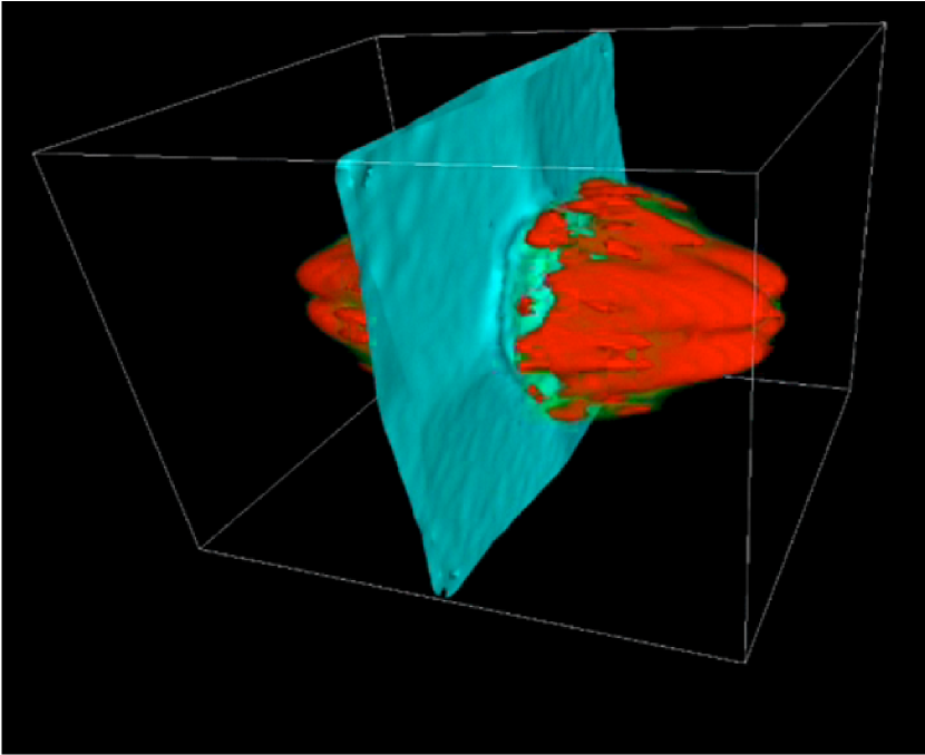
Figure 2: Snapshot of a hydrodynamical simulation of an explosion inside a cosmological pancake. Blue: density isosurface, showing the pancake. Notice the circular ripple resulting from the explosion. Red: temperature isosurface, showing the outflow.

This expression contains no linear terms since the density is a local maximum. In practice, we consider the density distribution inside a sphere of radius, $R^{*}$, centered on the point, $P$, and perform a least-square fit of equation (1) to determine numerically the values of the 6 coefficients $A$, $B$, $C$, $D$, $E$, $F$. Once these coefficients are determined, we rotate to a new coordinate system $(x^{\prime},y^{\prime},z^{\prime})$, such that the the cross-terms vanish. Equation (1) reduces to

$$\delta(x^{\prime},y^{\prime},z^{\prime})=\delta_{\rm peak}-A^{\prime}{x^{\prime}}^{2}-B^{\prime}{y^{\prime}}^{2}-C^{\prime}{z^{\prime}}^{2}\,.$$ (2)

It is actually straightforward to perform this change of coordinates. We combine the coefficients of equation (1) to form the following matrix,

$$M=\left[\matrix{A&D&E\cr D&B&F\cr E&F&C\cr}\right]\,.$$ (3)

We then diagonalize this matrix. Since this matrix is real and symmetric, all three eigenvalues are real. These eigenvalues are the coefficients $A^{\prime}$, $B^{\prime}$, $C^{\prime}$, respectively, and the 3 corresponding eigenvectors give us the directions of the three coordinate axes $x^{\prime}$, $y^{\prime}$, and $z^{\prime}$, respectively.

The three coefficients $A^{\prime}$, $B^{\prime}$, and $C^{\prime}$ are always positive, otherwise the point, $P$, would not be a maximum, but rather a saddle point or a minimum. Each coefficient is a measure of how fast the density drops as we move away from the peak in the direction corresponding to that coefficient. Therefore, the largest coefficient corresponds to the direction along which the density drops the fastest. We will interpret this as being the direction of least resistance, and assume that the outflow will naturally follow that direction. For instance, if $B^{\prime}$ happens to be the largest of the 3 coefficients, then the outflow will be directed along the $y^{\prime}$-axis.

2.3 The Expansion of the Outflow

In this section, we present the equations describing the expansion of the outflow. The technique used for solving these equations is shown in Appendix A.

2.3.1 Basic Equations

Tegmark, Silk, & Evrard (1993, hereafter TSE) presented a formulation of the expansion of isotropic outflows that was based on previous work by numerous authors (Cox & Smith, 1974; McKee & Ostriker, 1977; Weaver et al., 1977; McCray & Snow, 1979; Bruhweiler et al., 1980; Tomisata, Habe, & Ikeuchi, 1980; McCray & Kafatos, 1987; Ostriker & McKee, 1988) and refined it to account for the expansion of the universe. In this formulation, the injection of thermal energy produces an outflow of radius, $R$, which consists of a dense shell of thickness $R\delta$ containing a cavity. A fraction, $1-f_{m}$, of the gas is piled up in the shell, while a fraction, $f_{m}$, of the gas is distributed inside the cavity. We normally assume $\delta\ll 1$, $f_{m}\ll 1$, that is, most of the gas is located inside a thin shell. This is called the thin-shell approximation.

The original equations of TSE have been refined by several authors (Madau, Ferrara, & Rees 2001; SB01; Scannapieco, Ferrara, & Madau 2002, hereafter SFM) to include various additional physical processes. Hence, there is not a “unique” form of the equations. In this paper, the evolution of the shell radius, $R$, expanding out of a halo of mass, $M$, is described by the following system of equations,

$$\ddot{R} = {8\pi G(p-p_{\rm ext})\over\Omega_{b}H^{2}R}-{3\over R}(\dot{R}-HR)^{2}-{\Omega H^{2}R\over 2}-{GM\over R^{2}}\,,$$ (4)

$$\dot{p} = {L\over 2\pi R^{3}}-{5\dot{R}p\over R}\,,$$ (5)

where a dot represents a time derivative, $\Omega$, $\Omega_{b}$, and $H$ are the total density parameter, baryon density parameter, and Hubble parameter at time, $t$, respectively, $L$ is the luminosity (discussed in §2.3.3), $p$ is the bubble pressure resulting from this luminosity, and $p_{\rm ext}$ is the external pressure of the IGM. The four terms in equation (4) represent, from left to right, the driving pressure of the outflow, drag due to sweeping up the IGM and accelerating it from velocity $HR$ to velocity $\dot{R}$, and the gravitational deceleration caused by both the expanding shell and the halo itself. The two terms in equation (5) represent the increase in pressure caused by injection of thermal energy, and the drop in pressure caused by the expansion of the outflow, respectively. For details, we refer the reader to Ostriker & McKee (1988) and TSE.

These expressions most closely resemble that of SFM, the one difference coming from their use of a radially dependent mass in the last term of equation (4), derived by assuming a NFW profile (Navarro, Frenk, & White, 1997). This is motivated by the gravitational drag on a spherical outflow expanding out of a spherical collapsed halo, and is no longer an adequate description in the case being examined since an anisotropic outflow will more rapidly escape an elliptical halo. The influence of the gravitational potential well will be an intermediate case between this and a point mass. In practice we take the simpler form by assuming a point mass, as in SB01. We justify this approximation as follows: early in the outflow lifetime the effect of gravity on the outflow is negligible compared to other effects (see Appendix A). As the outflow expands, the gravity terms eventually become important, by which time most outflows have left the halo from which they originate. Notice that the original formulation of TSE did not include the term $-GM/R^{2}$, and also ignored the external pressure $p_{\rm ext}$.

These equations provide a full description of isotropic outflows. We now modify these equations to describe anisotropic outflows with any value of the opening angle, $\alpha$. We impose the condition that the modified equations reduce to equations (4) and (5) in the isotropic limit $\alpha=180^{\circ}$.

First consider equation (5). The two terms in the right hand side correspond to the increase in pressure caused by thermal energy injection, and the decrease in pressure caused by the expansion of the outflow, respectively. At this point, we need to backtrack. Equation (5) was derived from the following system of equations (TSE):

$$E_{t} = {3pV\over 2}\,,$$ (6)

$$\dot{E}_{t} = L-p\dot{V}\,,$$ (7)

where $E_{t}$ is the thermal energy inside the outflow, and $V$ is the volume of the outflow. We take the time derivative of equation (6), and eliminate $\dot{E}_{t}$ using equation (7). We get

$$\dot{p}={2L\over 3V}-{5p\dot{V}\over 3V}\,.$$ (8)

If we now substitute $V=4\pi R^{3}/3$, we recover equation (5). However, a bipolar anisotropic outflow with opening angle, $\alpha$, has a volume given by

$$V={4\pi R^{3}\over 3}\left(1-\cos{\alpha\over 2}\right)\,.$$ (9)

We substitute equation (9) in equation (8), and get

$$\dot{p}={L\over 2\pi R^{3}[1-\cos(\alpha/2)]}-{5\dot{R}p\over R}\,.$$ (10)

Physically, as $\alpha$ decreases, the energy is injected in a smaller volume, resulting in a larger pressure, $p$. This equation replaces equation (5). In our model, this is the only modification we need to make to the equations describing the expansion of the outflow (although a modification to the luminosity will be required). Equation (4) remains unchanged.

2.3.2 The External Pressure

The external pressure, $p_{\rm ext}$, depends upon the density and temperature of the IGM, which can be quite complex. But in the context of the analytic approximation we are using, we are justified in making some simplifying approximations. Following Madau, Ferrara, & Rees (2001), we will assume a photoheated IGM with a fixed temperature, $T_{\rm IGM}=10^{4}{\rm K}$. We will also assume an IGM density, $\rho_{\rm IGM}$, equal to the mean baryon density, $\bar{\rho}_{b}$. Hui & Gnedin (1997) performed detailed hydrodynamical calculations of the equation of state for a photoheated IGM, and showed that the temperature is a function of the density. But according to their Figure 1, a temperature of $10^{4}{\rm K}$ is appropriate for densities, $\rho\approx\bar{\rho}_{b}$. It should also be noted that the temperature of the IGM is redshift-dependent as shown by Schaye et al. (2000) and we will neglect this here. Our choice of fixed external temperature and density will be discussed further in §5. The external pressure is then given by

$$p_{\rm ext}(z)={\bar{\rho}_{b}kT_{\rm IGM}\over\mu}={3\Omega_{b,0}H_{0}^{2}kT_{\rm IGM}(1+z)^{3}\over 8\pi G\mu}\,,$$ (11)

where $z$ is the redshift, $\mu$ is the mean molecular mass, and subscripts 0 indicate present values. The value of $\mu$ depends upon the ionization state of the gas. We assume that hydrogen is ionized (Page et al., 2006) and helium is singly-ionized in the redshift range $3<z<7$ (Theuns et al., 2002a; Choudhury & Ferrara, 2005), which is most of the redshift range in which our outflows are actively expanding. Also, even when much of the IGM is still neutral, it is reasonable to expect the source galaxy to have photoionized the region ahead of the outflow. We will assume that this is the case throughout the simulations. The mean molecular weight is then $\mu=2/(4-3Y)\,{\rm a.m.u.}$ (atomic mass units). For a helium abundance, $Y=0.242$ (Izotov & Thuan, 2004), we get $\mu=0.611\,{\rm a.m.u.}$.

2.3.3 The Luminosity

The luminosity, $L$, is the rate of energy deposition or dissipation within the outflow and is a sum of five terms,

$$L(t)=L_{\rm SN}-L_{\rm comp}-L_{\rm ne^{2}}-L_{\rm ion}+L_{\rm diss}\,,$$ (12)

where $L_{\rm SN}$ is the total luminosity of the supernovae responsible for generating the outflow, $L_{\rm comp}$ represents the cooling due to Compton drag against CMB photons, $L_{\rm ne^{2}}$ represents the cooling due to 2-body interactions, $L_{\rm ion}$ represents the cooling due to ionization, and $L_{\rm diss}$ represents heating from collisions between the shell and the IGM. Following SFM, we will assume that the first two terms, supernovae and Compton drag, dominate, and will neglect the remaining terms. The supernovae luminosity, for a galaxy forming in a halo of mass, $M$, is given by

$$L_{\rm SN}={f_{\rm w}E_{0}\over t_{\rm burst}}{M_{*}\over M_{\rm req}}=2.86f_{\rm w}f_{*}\left({\Omega_{b,0}\over\Omega_{0}}\right)\left({M\over 1{\rm M}_{\odot}}\right)\,{\rm L}_{\odot}\,,$$ (13)

where $f_{\rm w}$ is the fraction of the total energy released that goes into the outflow, $f_{*}$ is the star formation efficiency, and the total mass in stars formed during the starburst is $M_{*}=f_{*}M\Omega_{b,0}/\Omega_{0}$. $M_{\rm req}$ is the mass of stars required to form one SN and we take a value of $M_{\rm req}=89.7{\rm M_{\odot}}$ (derived using a broken power-law IMF from Kroupa 2001) and the energy released by each of these SNe is $E_{0}=10^{51}{\rm ergs}$. Leitherer & Heckman (1995) show that for instantaneous star formation, as considered here, the SN outflow phase associated with this burst last for a duration of $t_{\rm burst}=5\times 10^{7}{\rm yr}$ and the delay before the first SNe is negligible. We use the galaxy mass dependent determination of $f_{\rm w}$ given by SFM, $f_{\rm w}(M)=0.3\delta_{B}(M)/\delta_{B}(M=2\times 10^{8}{\rm M_{\odot}})$, where

$$\delta_{B}(M)=\cases{1.0,&$\tilde{N}_{t}\leq 1$;\cr 1.0+0.165\ln(\tilde{N}_{t}^{-1}),&$1\leq\tilde{N}_{t}\leq 100$;\cr\left[1.0-0.165\ln(100)\right]100\tilde{N}_{t}^{-1},&$100\leq\tilde{N}_{t}$;\cr}$$ (14)

and $\tilde{N}_{t}\equiv 1.7\times 10^{-7}({\Omega_{b,0}/\Omega_{0}})M/(1{\rm M_{\odot}})$.

The ionization state inside the outflow is even more uncertain and may be a function of distance from the source as the gas may recombine as it expands from its source galaxy. Until we have a more precise model for the internal structure of the outflow, we will simply make the same assumption as for the surrounding IGM: ionized hydrogen and singly-ionized helium. However, it is worth noting that the extreme case, where outflows contain fully ionized gas, involves only a minor modification of the Compton drag. Following TSE, the Compton luminosity is given by

$$L_{\rm comp}={\pi^{2}\over 15}(\sigma_{t}cn_{e})\left({kT_{e}\over m_{e}c^{2}}\right)(kT_{\gamma})^{4}{V\over(\hbar c)^{3}}\,,$$ (15)

where $\sigma_{t}$ is the Thompson cross section, $T_{\gamma}$ is the CMB temperature, and $n_{e}$ and $T_{e}$ are the electron number density and temperature inside the bubble, respectively. The pressure, $p$, inside the bubble is given by

$$p=nkT_{e}=(n_{e}+n_{\rm ion})kT_{e}V\,.$$ (16)

We assume that hydrogen is ionized and helium is singly-ionized and hence $n_{\rm ion}=n_{e}$, which is also the approximation made in TSE. Equation (16) becomes $n_{e}kT_{e}=p/2$. We now eliminate $n_{e}kT_{e}$ in equation (15). We also eliminate $V$ using equation (9), and get

$$L_{\rm comp}={2\pi^{3}\over 45}{\sigma_{t}\hbar\over m_{e}}\left({kT_{\gamma 0}\over\hbar c}\right)^{4}\left(1-\cos{\alpha\over 2}\right)(1+z)^{4}pR^{3}\,,$$ (17)

where $T_{\gamma 0}$ is the present CMB temperature. We used $T_{\gamma}=T_{\gamma 0}(1+z)$, which is valid over the range of redshifts we consider.

2.3.4 The Final Stage of the Outflow

The expansion of the outflow is initially driven by the supernovae luminosity. After the supernovae turn off, the outflow enters the “post-supernova phase.” The pressure inside the outflow keeps driving the expansion, but this pressure drops since there is no energy input from supernovae. Eventually, the pressure will drop down to the level of the external IGM pressure. At that point, the expansion of the outflow will simply follow Hubble expansion. Since we assume identical mean molecular weights inside and outside the outflow, the condition $p=p_{\rm ext}$ implies $T=T_{\rm IGM}=10^{4}{\rm K}$.

Figure 3 shows the isotropic outflow solution for a halo of mass, $M=2.8\times 10^{9}{\rm M}_{\odot}$ that collapses at redshift, $z=8.10$, in a $\Lambda$CDM universe. The cooling time is short, $3{\rm Myr}$, so the galaxy forms soon after, at $z=8.07$. The outflow turns on immediately, as discussed in the previous section, and goes on to form the largest outflow in our simulations.

Figure 3: Evolution of the largest outflow. The middle panel shows the comoving radius of the outflow versus redshift, $z$. The thick lines separate the various phases of the expansion (supernova-driven, post-supernova, Hubble expansion). The top panel shows the total luminosity, $L=L_{\rm SN}-L_{\rm comp}$, versus redshift. The bottom panel shows the external IGM pressure (solid line) and the pressure of the outflow (dotted line).

The top panel shows the total luminosity, and the middle panel shows the comoving radius. The bottom panel shows the pressure, $p$, of the outflow and the external pressure, $p_{\rm ext}$, of the IGM. Initially, during the supernova phase, the outflow is driven by the energy input from supernovae and the radius steadily increases. During this phase, the supernova luminosity, $L_{\rm SN}$, exceeds the Compton luminosity by factors of several and for this particular outflow dominates it entirely. The pressure diverges at the redshift of supernova turn-on (because we neglect the finite volume of the region containing the supernovae), but then drops as $t^{-4/5}$ (see Appendix A). At $z=7.63$, the supernovae burn out, and the only contribution to the total luminosity is the energy loss by Compton drag. The outflow enters the post-supernova phase. The turn-off of the supernovae produces a change of slope in the pressure, which in turn produces a change of slope in the Compton luminosity. The post-supernova phase lasts until redshift $z=4.95$. At that point, the pressure of the outflow becomes equal to the external pressure, and the outflow switches to pure Hubble expansion.

3 THE MONTE CARLO METHOD

We use essentially the same Monte Carlo method as in SB01, generalized to include anisotropic outflows. In our dynamical equation for the evolution of the outflow [eq. (4)], we include the external pressure, $p_{\rm ext}$, an effect that was neglected in SB01, but included in SFM.

3.1 Cosmological Model and Initial Conditions

We consider a $\Lambda$CDM model with present density parameter, $\Omega_{0}=0.27$, baryon density parameter, $\Omega_{b,0}=0.04444$, cosmological constant, $\lambda_{0}=0.73$, Hubble constant, $H_{0}=71\rm\,km\,s^{-1}Mpc^{-1}$ ($h=0.71$), primordial tilt, $n_{s}=0.93$, and CMB temperature, $T_{\rm CMB}=2.725$, consistent with the results of WMAP (Bennett et al., 2003). We simulate structure formation inside a comoving cubic volume of size, $L_{\rm box}=12h^{-1}{\rm Mpc}$, with periodic boundary conditions. To generate initial conditions, we lay down a cubic grid of size $512\times 512\times 512$ in the computational volume, and compute the initial density contrast, $\delta_{i}$, at initial redshift, $z_{i}=24$. We also compute, on 10 similar grids, the same density contrast, but filtered at the 10 mass scales: $M_{1},M_{2},\ldots,M_{10}$. As we use a Gaussian filter, the mass, $M$, and comoving radius, $R_{f}$, of the filter are related by $M=(2\pi)^{3/2}R_{f}^{3}\bar{\rho}_{0}$, where $\bar{\rho}_{0}=3\Omega_{0}H_{0}^{2}/8\pi G$ is the present mean density of the universe. The values of the mass and length filtering scales are listed in Table 1. The last two columns indicate the filtering radius in units of the grid spacing, $\Delta$, and in units of the box size, $L_{\rm box}$.

Table 1: Mass and Length Filtering Scales

Filter name	$M\;[{\rm M}_{\odot}]$	$R_{f}\;[{\rm kpc}]$	$R_{f}/\Delta$	$R_{f}/L_{\rm box}$
M01	7.61${}\times 10^{7}$	50.4	1.53	0.00299
M02	2.53${}\times 10^{8}$	75.2	2.28	0.00445
M03	8.42${}\times 10^{8}$	112.3	3.40	0.00664
M04	2.80${}\times 10^{9}$	167.6	5.08	0.00992
M05	9.32${}\times 10^{9}$	250.2	7.58	0.0148
M06	3.10${}\times 10^{10}$	373.6	11.31	0.0221
M07	1.03${}\times 10^{11}$	557.8	16.90	0.0330
M08	3.43${}\times 10^{11}$	832.7	25.23	0.0493
M09	1.14${}\times 10^{12}$	1243.1	37.66	0.0736
M10	3.80${}\times 10^{12}$	1855.9	56.22	0.110

The method for generating these 11 grids is described in great detail by Martel (2005). Essentially, we work in $k$-space, by generating, on a $512^{3}$ grid, the density harmonics, $\hat{\delta}(k)$, corresponding to a $\Lambda$CDM power spectrum at $z=z_{i}=24$. Once the density harmonics are generated we take the inverse Fourier transform to obtain the initial density contrast, $\delta_{i}$. This gives us our first grid in real space, with the unfiltered density contrast. To get the 10 filtered grids, we first multiply the density harmonics by the Fourier transform of the filter, and then take the inverse Fourier transform to get the filtered density contrast. Notice that in our simulations the value of the initial redshift, $z_{i}$, is actually irrelevant, as long as it is larger than the collapse redshifts of all the density peaks that are resolved in our simulations. It turns out that the first peak collapses at redshift, $z=18.55$.

3.2 The Local Density Peaks

For each of the 10 filtered grids, we identify the location of the local density peaks. These peaks are defined as grid points where the density contrast is positive, and its value exceeds the values at the 26 neighboring grid points (taking periodic boundary conditions into account). For each density peak on each filtered grid, we compute a collapse redshift, $z_{\rm coll}$, and a direction of least resistance, $\hat{\bf e}$. The collapse redshift is obtained by solving numerically the following equation,

$$\delta_{c}(z_{\rm coll})=\delta_{i}{\delta_{+}(z_{\rm coll})\over\delta_{+}(z_{i})}\,,$$ (18)

where $\delta_{i}$ is the initial density contrast at the peak, and $\delta_{+}$ is the linear growing mode (for flat, $\Lambda\neq 0$ models, see, e.g., Martel 1991, equation [18]). The critical value, $\delta_{c}$, is equal to 1.69 for an Einstein-de Sitter model, and slowly varies with redshift for other models. In our simulations, we simply assume $\delta_{c}=1.69$. If equation (18) has no solution, we are simply dealing with a density peak that would collapse in the future, and we just ignore it.

To check for consistency, we performed a N-body simulation of structure formation in a box of the same size, for the same cosmological model and density fluctuation power spectrum. We used a $\rm P^{3}M$ algorithm (Hockney & Eastwood, 1981) with $256^{3}$ equal-mass particles. The mass per particles was $1.087\times 10^{7}{\rm M}_{\odot}$, hence the lowest mass scale $M_{1}$ corresponds to 7 particles which, though insufficient for determining the halo density profile, is fine for the simple locating of halos that follows. We used a standard friends-of-friends algorithm (Davis et al., 1985) to identify halos at various redshifts between $z=24$ and $z=2$. For this, we used 2 different linking lengths. We first use the “standard” value $l=0.25\Delta x$, where $\Delta x$ is the mean particle spacing. We also used a value $l=(18\pi^{2})^{-1/3}\Delta x=0.1779\Delta x$, corresponding to a density increase by a factor of $18\pi^{2}$. This is consistent with the assumption that collapsed, virialized halos have a density equal to $18\pi^{2}$ times the mean background density (see eq. [19] below). Only halos containing 6 particles or more are included. This corresponds to a minimum mass of $6.522\times 10^{7}{\rm M}_{\odot}$.

In Figure 4, we plot the number of collapsed halos present in the N-body simulation versus redshift (dashed lines). We find more halos with $l=0.25$ than with $l=0.1779$. This might seem surprizing since halos “break up” as $l$ is reduced. However, many halos fall below the threshold of 6 particles when $l$ is reduced. The two methods differ by about 20% at low redshift, but the difference increases at high redshift. The dotted line shows a calculation based on the Press-Schechter (PS) approximation (Press & Schechter, 1974). The agreement with the N-body simulations is excellent at low redshift, while at very high redshifts ($z>15$) the PS approximation overestimates the number of halos. The solid line shows the number of collapsed halos in our Monte Carlo simulations. This was obtained by counting, at given redshifts $z$, the number of halos with $z_{\rm coll}>z$, and removing the halos that have been destroyed by mergers (see §3.4 below). The number of halos is lower for the Monte Carlo simulations than for the N-body simulation or the PS approximation, at almost all redshifts. We interpret this result as follows: in the Monte Carlo simulations, only the matter located in overdense regions can eventually end up inside collapsed halos, while in the N-body simulations, all the matter in the system can eventually end up in halos. Notice also that the comparison between the PS and N-body results, and the Monte Carlo results is complicated by the fact that the mass spectrum of halos is discrete for the Monte Carlo simulations. For the N-body simulation and the PS approximation, the choice of an appropriate minimum mass is not obvious, and the results are quite sensitive to that choice, especially at high redshift when most halos have a small mass.

Figure 4: Number of collapsed halos present in the computational volume, versus redshift. Long and short dashes: N-body simulation with friends-of-friends algorithm, with linking lengths, $l=0.25\Delta x$ and $l=0.1779\Delta x$, respectively; dotted line: Press-Schechter approximation;solid line: Monte Carlo simulations.

These results also vindicate our choice of an initial redshift of, $z_{i}=24$. Clearly the system is still in the linear regime at that redshift. The very first halo collapses at redshift $z=18.55$ in the Monte Carlo simulations, and at redshifts, $z=16-17$, in the N-body simulation, while the PS approximation predicts that a computational volume of that size will typically contain one halo at $z=19$. Indeed, the probability of finding one halo of mass, $M=M_{1}=7.61\times 10^{7}{\rm M}_{\odot}$, at $z=24$, according to the PS approximation, is about 1/1000.

3.3 The Direction of Least Resistance

We compute, for each peak, the direction of least resistance, using the method described in §2.2. The radius, $R^{*}$, defines the region around the peak over which the least-square fit to equation (1) is performed. Its value will affect the determination of the coefficients, $A$, $B$, $C$, $D$, $E$ and $F$, and ultimately the direction, $\hat{\bf e}$, of the outflow. The largest possible value of $R^{*}$ should be the filtering scale, since this scale corresponds to the physical extent of the peak (using a larger value would amount to including matter that belongs to different peaks). As for the minimum value, $R^{*}$ must clearly be at least equal to the grid spacing, $\Delta$. It turns out that this condition is insufficient. If $R^{*}<2^{1/2}\Delta$, only the 6 nearest grid points to the peak are included in the fit. In that case, the matrix, $M$, is already diagonal, and the only directions allowed for the outflow are along the unrotated coordinate axes $x$, $y$, $z$. We must at least include the 12 next nearest grid points, located at a distance equal to $2^{1/2}\Delta$ from the peak.

To test how the direction of the outflow depends on the particular choice of $R^{*}$, we considered the filters, M03, M04, $\ldots$, M10, and computed, for all peaks, two values of $\hat{\bf e}$: one using $R^{*}=2\Delta$, and one using $R^{*}$ equal to the filtering scale, $R_{f}$. Figure 5 shows histograms of the angle in degrees between these two values of $\hat{\bf e}$. We excluded from this test the mass filters M01 and M02, because the range of allowed values for $R^{*}$ becomes very narrow, and there is essentially no uncertainty in these cases.

Figure 5: Histograms of the fluctuations in the direction of the outflows resulting from variations in $R^{*}$. Notice that the last two bins correspond to the ranges [10,15] degrees and [15,90] degrees, respectively. The labels in the panels indicate the mass filtering scale and the number of peaks.

For the vast majority of peaks, the angle is below 4 degrees and it exceeds 10 degrees only for very few peaks. The interpretation of these results is that our method for determining the direction of the outflow has an uncertainty of a few degrees, resulting from the ambiguity in the choice of $R^{*}$. In the limit when the opening angle of the outflow is much larger than that uncertainty, the region of space containing the outflow is essentially unchanged. We will consider opening angles of several tens of degrees, while the uncertainty in the direction of least resistance is of order a few degrees. The final results might vary by a few percent as a result, but this is not sufficiently large to be the dominant source of error.

From this test, we conclude that our technique for determining the direction of least resistance is robust, and consequently the particular value chosen for $R^{*}$ is not important. Hence, we decided to set $R^{*}$ equal to the filtering scale, $R_{f}$.

Once this is all done, we have, for each of the 10 filtering scales, a list of local density peaks, and for each of these peaks, a position, ${\bf r}$, a mass, $M$ (the mass of the corresponding filtering scale), a collapse redshift, $z_{\rm coll}$, and a direction of least resistance, $\hat{\bf e}$. In the model, each peak corresponds to a density fluctuation of mass, $M$ (the filtering mass), and radius, $R_{f}$ (the filtering radius). If left alone, this peak will collapse at redshift, $z_{\rm coll}$, to form a halo of mass, $M$, located at position, ${\bf r}$. This protogalaxy will eventually turn into a galaxy (by forming stars), and generate an outflow propagating along the direction of least resistance, $\hat{\bf e}$.

3.4 Formation of First-Generation Galaxies

The 10 filtered grids represent the same region of the universe. Hence, we cannot simply assume that every peak collapses to form a protogalaxy, since this would violate conservation of mass. We must deal with the issue of halos inside halos. Consider two density peaks $a$ and $b$ of masses, $M_{a}<M_{b}$ (these peaks are therefore on different grids). If the separation, $|{\bf r}_{a}-{\bf r}_{b}|$, between the peaks is smaller than the filtering scale, $R_{f,b}$, of the larger mass, the two halos that these peaks will form cannot coexist, since the smaller halo is inside the larger one. There are then two possibilities, depending on the collapse redshifts. If $(z_{\rm coll})_{b}>(z_{\rm coll})_{a}$, then halo $a$ will never form, since all the matter it contains will be incorporated into halo $b$, that forms earlier. While this does occur it is not common, since in a CDM universe smaller peaks tend to collapse earlier than bigger ones. The second possibility is $(z_{\rm coll})_{a}>(z_{\rm coll})_{b}$. In this case, halo $a$ will form first, at redshift $(z_{\rm coll})_{a}$, but will be destroyed later by a merger event at redshift, $(z_{\rm coll})_{b}$, that results in the formation of halo $b$. So, even though halos remain at fixed locations in this simplified Monte Carlo model, non-dynamic merger events are included.

The collapse of a peak leads to the formation of a halo, which we identify as a protogalaxy. The gas inside that halo is at the virial temperature, given by

$$T_{\rm vir}={0.009\,{\rm K}\over\beta}\left({6.8\over 5X+3}\right)\left({Mh\over 1\,{\rm M}_{\odot}}\right)^{2/3}(1+z_{\rm coll})\left[{\Omega_{0}\over\Omega(z_{\rm coll})}\right]^{1/3}\left[{\Delta_{c}(z_{\rm coll})\over 18\pi^{2}}\right]^{1/3}\,,$$ (19)

(Eke, Cole, & Frenk, 1996), where $X=0.76$ is the hydrogen mass fraction, and $\Delta_{c}$ is the ratio of the halo’s mean density to the critical density. Since this temperature is usually much too high to allow the formation of stars, the gas must cool down to a temperature, $T\ll T_{\rm vir}$, before stars form and the protogalaxy becomes a galaxy. As in SB01, we use the cooling model of White & Frenk (1991). This model assumes that the cooling proceeds inside-out. The gas inside a “cooling radius,” $r_{\rm cool}$, has cooled, while the gas outside $r_{\rm cool}$ remains hot. As $r_{\rm cool}$ increases with time, the mass, $M_{\rm cool}$, of cool gas increases, until all the gas has cooled. The mass, $M_{\rm cool}$, evolves according to

$${dM_{\rm cool}\over dt}=12\left({\Omega_{b,0}\over\Omega_{0}}\right)^{3/2}f_{0}\left({T_{\rm vir}\over 1\,{\rm K}}\right)\left[\Lambda_{23}(T_{\rm vir},Z)\right]^{1/2}\left({t\over 1\,{\rm yr}}\right)^{-1/2}M_{\odot}\,{\rm yr}^{-1}\,,$$ (20)

where $\Lambda_{23}$ is the cooling rate in units of ${\rm 10^{-23}ergs\,s^{-1}cm^{-3}}$, which is a function of temperature and metallicity, $Z$, and $f_{0}\approx 0.8$ [a correction factor suggested by Somerville (1997) to bring this result into line with more complex analyses]. We determine the required cooling rate using MAPPINGS III, a successor to MAPPINGS II outlined in Sutherland & Dopita (1993). We integrate both sides between $t=0$ and $t=t_{\rm cool}$, the cooling time. For a halo of mass, $M$, and gas mass, $M_{\rm gas}=\Omega_{b,0}M/\Omega_{0}$, we get

$$t_{\rm cool}={1\over 576f_{0}^{2}}\left({M\over 1{\rm M}_{\odot}\,}\right)^{2}\left({\Omega_{b,0}\over\Omega_{0}}\right)^{-1}\left({T_{\rm vir}\over 1\,{\rm K}}\right)^{-2}\left[\Lambda_{23}(T_{\rm vir},Z)\right]^{-1}{\rm yr}\,.$$ (21)

Using the solution of the Friedman equation for our $\Lambda$CDM model, we compute, for each halo, the epoch, $t_{\rm coll}$, at which collapse occurs from the collapse redshift, $z_{\rm coll}$. We then add the cooling time to get the epoch at which galaxy formation occurs, $t_{\rm gf}=t_{\rm coll}+t_{\rm cool}$, and compute the corresponding galaxy formation redshift, $z_{\rm gf}$. The galaxy formation epoch may be later than the current epoch, in which case stars will not form and the halo will remain a protogalaxy, unless metal deposition from outflows modifies the cooling rate (see below).

We refer to these galaxies as “first-generation” galaxies since at the time of formation they are untouched by impinging outflows from other galaxies. For these galaxies we assume a cooling rate based on zero metallicity. In the following section we will discuss galaxies for which this is not the case.

We are now ready to proceed with the simulation. Starting at initial redshift $z_{i}=20$ (since there are no collapsed halos at higher redshift), we evolve the system forward by redshift steps of $\Delta z=-0.005$. As a result we take 3600 steps to reach the end point for our simulations, which is $z=2$. This end point is chosen for comparison with Quasar absorption spectra data from $z=2-6$. Also, our box would no longer represent a cosmological volume at lower redshifts.

At the location of peak, $a$, a halo forms at redshift, $(z_{\rm coll})_{a}$, unless that peak was located inside a larger peak that collapsed first, as described above. During the redshift interval, $[(z_{\rm coll})_{a},(z_{\rm gf})_{a}]$, while the gas is cooling, the halo might be destroyed by a merger. This will happen if there is a peak $b$ for which

$$M_{b}>M_{a}\,,$$ (22)

$$(z_{\rm coll})_{a}>(z_{\rm coll})_{b}>(z_{\rm gf})_{a}\,,$$ (23)

$$|{\bf r}_{a}-{\bf r}_{b}|<R_{f,b}\,.$$ (24)

In this case, the halo was able to form, but did not manage to cool before being destroyed, hence the actual galaxy never formed.

If the galaxy does manage to form, we neglect the formation time and life span of massive stars and so the newly formed galaxy immediately produces an outflow centered at the halo position, ${\bf r}_{a}$, and propagating along the direction, $\hat{\bf e}_{a}$. We evolve this outflow with time, using the solutions given in Appendix A (with timesteps corresponding to our redshift steps, $\Delta z=-0.005$).

Left alone, the outflow will go through successive phases of driven expansion by supernovae and near-adiabatic expansion driven by pressure alone before joining the Hubble flow. However, during either of these stages, the galaxy producing the outflow might be destroyed by a merger. In all such cases the outflow reverts to a Hubble expansion phase.

3.5 Subsequent Galaxy Formation

After the first outflows are formed, some will begin to strike other density peaks and modify the way these systems evolve. They may enrich these systems with new metals, possibly modifying their cooling time. They may also expel the gas content of the object by ram pressure stripping or shock-heating of the gas. Of these two mechanisms, the former (stripping) is the dominant one (Scannapieco, Ferrara, & Broadhurst, 2000) and so we will neglect the latter.

3.5.1 Stripping

Density peaks may be stripped of their baryons when the swept-up shell of intergalactic and interstellar gas incident upon them imparts sufficient momentum on the baryons such that they escape the potential well of the peak, i.e.

$$\left({l^{2}\over 4R^{2}}\right)M_{o}v_{o}\geq M_{b}v_{\rm esc},$$ (25)

where the mass of the swept up shell is $M_{o}$ at radius, $R$, (as in TSE), $v_{o}$ is the outflow velocity, $M_{b}$ is the baryonic mass of the density peak struck, and $v_{\rm esc}$ is the escape velocity for successfully stripped gas. $l$ is the comoving radius of the collapsing density peak. Using the spherical approximation for gravitational collapse, this scale is determined from the non-linear density contrast, $\delta_{\rm NL}$ using $l=R_{f}(1+\delta_{\rm NL})^{-1/3}$ where $1+\delta_{\rm NL}=9(\theta-\sin\theta)^{2}/[2(1-\cos\theta)^{3}]$. The parameter, $\theta$, is in turn given by

$$\left(\theta-\sin\theta\over 2\pi\right)^{2/3}={\delta_{+}(z)\over\delta_{+}(z_{\rm coll})}\,,$$ (26)

where $\delta_{+}(z_{\rm coll})$ and $\delta_{+}(z)$ are the linear growing modes at collapse and when the outflow strikes the peak respectively.

We assume that stripping may only occur for systems that have not collapsed since the cross section to impact is small and would result in negligible momentum transfer. This approach is supported by Sigward, Ferrara, & Scannapieco (2005) who investigate this issue with a numerical analysis of an individual object struck by a shock. It is also worth noting that we deal with baryonic stripping in the same way whether or not the source galaxy is within the filtering radius of the density peak struck (although it is less likely to occur due to the larger escape velocity and mass of the halo struck).

When the criterion for stripping is met, the density peak is rendered free of baryons and, while it may collapse, it will not form a galaxy. If the shell of the outflow does not strip the peak then the peak is enriched by the metal-rich gas, which fills the outflow.

3.5.2 Metal Enrichment

Metals are propagated throughout our simulations within the hot bubbles of outflows. Peaks that have not been struck by outflows are assumed to have metallicity of $\rm[Fe/H]=-3$, which is negligible for the purposes of calculating the halo cooling time. Once galaxies are formed metals are produced at rate of $2{\rm M_{\odot}}$ per SN (Nagataki & Sato, 1998). Hence the mass of metals in the outflow is

$$M_{Z}=f_{\rm esc}{2{\rm M_{\odot}}\over M_{\rm req}}f_{*}{\Omega_{b,0}\over\Omega_{0}}M\,,$$ (27)

where $f_{\rm esc}$ is the fraction of ISM gas blown out with the outflow. We use the value $f_{\rm esc}=0.5$ taken from the numerical simulations of Mori, Ferrara, & Madau (2002). This mass of metals is distributed evenly throughout the volume of the outflow.

It is notable that, in this model, the ratio of the mass lost rate to star formation rate is approximately $f_{\rm esc}/f_{*}=5$. This is consistent with observations that indicate this ratio is of order 1 for local starburst galaxies (e.g. Martin 1999 and Heckman et al. 2000), infrared-luminous galaxies (e.g. Rupke et al. 2005) and high-$z$ galaxies (e.g. Pettini et al. 2000).

When an outflow strikes an uncollapsed density peak and does not strip it, it modifies its metal content. It deposits a fraction of its metals, $f_{\rm dep}V_{\rm overlap}/V_{\rm outflow}$, where $f_{\rm dep}$ is a mass deposition efficiency, which we set at $f_{\rm dep}=0.9$, $V_{\rm overlap}$ is the volume of overlap of the uncollapsed density peak of radius $l$, and $V_{\rm outflow}$ is the volume of the outflow. This volume of overlap is calculated based on various geometric approximations to the overlap of two spherical cones and a sphere, depending on their relative size and orientation. Once the halo has collapsed, the addition of metals results in an increase in cooling rate and so a reduction in the cooling time, expediting galaxy formation.

We assume that the SNe in our simulations are only of the Type II variety since these SNe explode together shortly after the starburst and lead to a coherent extragalactic outflow that will reach large distances. As a result we use an alpha-element-rich yield of metals [quoted in Sutherland & Dopita (1993) as “primordial” abundance ratios] and distribute our mass of metals accordingly. This provides a value for ${\rm[Fe/H]}$ used to calculate the new cooling rate.

There is a special case to consider where a source galaxy is embedded in the density peak that its outflow strikes. In this case we assume the volume overlap of the outflow is 100% and so it will deposit a fraction, $f_{\rm dep}$, of its metals onto this structure. The main motivating factor behind the inclusion of this mass deposition efficiency is to avoid the implausible scenario that an outflow may continue to grow having left all its metals behind. The value it should take is unknown; however, the simulations are not sensitive to this factor, as we point out below.

4 RESULTS

4.1 The Impact of Varying Opening Angle

We have constructed a model for the evolution of anisotropic outflows and a test bed with which to investigate its significance and we are now ready to discuss what this approach tells us.

Taking an extreme case of anisotropy as an illustration, consider an opening angle of only $40^{\circ}$. At the natural end point of our simulations, $z=2$, Figure 6 shows a slice of thickness $0.4h^{-1}{\rm Mpc}$ through our simulation box. The position and extent of our galactic outflows are indicated along with the position and pre-collapse radius of peaks (i.e. the filtering scale, $R_{f}$, of the peak) that will collapse by $z=0$. These outflows extend a significant distance from their source galaxies and often strike other peaks. Where peaks are arranged in a row in the plane of the slice, the outflows appear to favor a direction perpendicular to this structure (see zoom in). This is to be expected: the locations of these galaxies trace the underlying structure of the dense filament out of which they form by fragmentation, and the outflows follow the path of least resistance away from that filament.

Figure 7 shows the counts of various quantities in units of $(h^{-1}{\rm Mpc})^{-3}$ by $z=2$, for varying opening angle. The number density of peaks that are hit by outflows that will go on to form halos by $z=0$ are shown. This decreases as approximately a power law for increasingly anisotropic outflows, which can be explained by two factors. Anisotropic outflows take a path of least resistance out of highly overdense regions and so will encounter fewer regions that go on to form halos. Also the total volume occupied by outflows is not conserved for varying opening angle since anisotropic outflows tend to overlap less (see above) and the volume per outflow is not constant. The degeneracy between these two effects is resolved in Figure 8 and the accompanying text. The number density of peaks stripped of their baryons is also shown and indicates that the fraction of peaks hit that are then stripped is roughly constant ($\sim 50\%$).

The number of galaxies formed by $z=2$ rises smoothly for decreasing opening angle in Figure 7 as a result of the fall in stripping. We find that metal enrichment of peaks has a negligible impact on the number of galaxies; however, those galaxies that form are born slightly earlier. Not all peaks that are hit by outflows but not stripped will go on to produce galaxies by $z=2$. This is because, despite being enriched by metals and collapsing, their baryons do not always cool to form stars by this redshift. As a result, the incidence of stripping decreases faster than the number of galaxies increases. This is demonstrated with the sum of these two number densities in Figure 7, which decreases with increasingly anisotropic outflows.

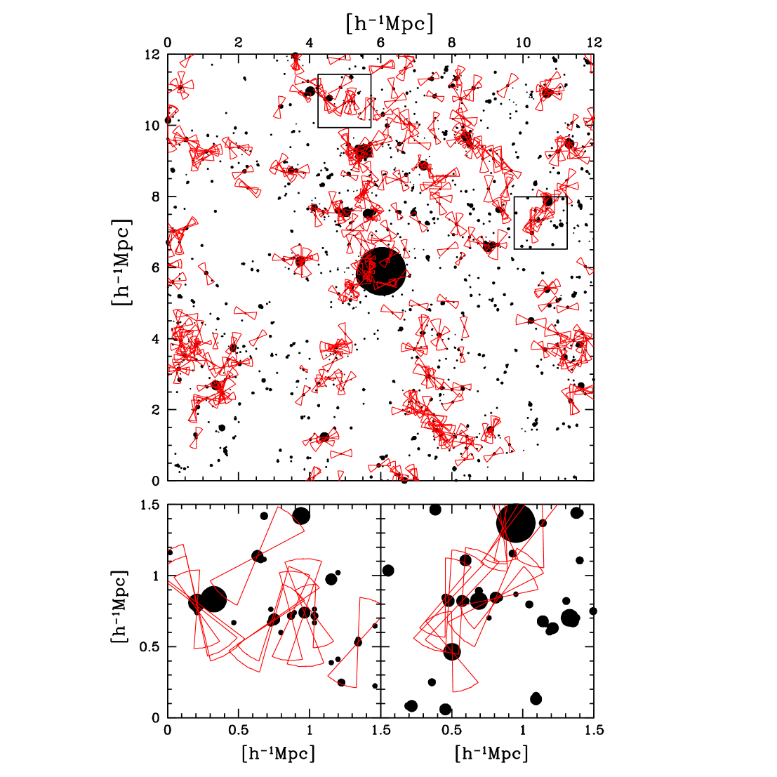
Figure 6: A slice through the simulation box of thickness $0.4h^{-1}{\rm Mpc}$ at $z=2$. Density peaks are shown as filled circles of diameter corresponding to their extent prior to collapse. The outflows have an opening angle of $40^{\circ}$, and their location and physical coverage are indicated as red wedges. Two zoom-in regions of size $1.5h^{-1}{\rm Mpc}$ show regions of interest, where galaxies that formed out of a common filament produce outflows that are aligned.

Figure 7: The number density of various objects in units $(h^{-1}{\rm Mpc})^{-3}$ at $z=2$, versus opening angle. Solid line: number of peaks hit that will go on to collapse before $z=0$; dotted line: number of those peaks that are then stripped of their baryons; short dashed line: number of galaxies; long dashed line: sum of the number of galaxies and stripped peaks.

In Figure 8 we show various statistics at $z=2$ in the simulations: the average distance, $\bar{R}_{\rm strip}$, traveled by outflows before stripping occurs, the maximum distance, $R_{\max}$, traveled by an outflow, the estimated volume filling factor of outflows, and the ratio of the number density of hits to the volume filling factor in units $(h^{-1}{\rm Mpc})^{-3}$. The mean distance traveled by outflows before stripping occurs is flat until the opening angle as low as $100^{\circ}$ where it begins to increase. As the anisotropic outflows travel farther with decreasing opening angle, they fail to hit new peaks as they have already escaped their highly overdense environments. It is only when $\alpha=100^{\circ}$ that they begin to reach the next dense structure.

Figure 8: Top left: mean radius of outflows when they strip peaks of their baryons; top right: the solid line shows the radius of the largest outflow and, for comparison, the dotted line shows $R\propto 1/[1-\cos{\alpha/2}]^{1/3}$, which is the relation expected if the volume enriched were conserved for varying opening angle. The estimated volume filling factor is shown in the bottom left panel; bottom right: the ratio of the number density of peaks hit to the volume filling factor in units of $(h^{-1}{\rm Mpc})^{-3}$.

In the top right panel we show the radius of the largest outflow for each opening angle. We also show a curve for constant volume using equation (9), which gives us $R\propto 1/[1-\cos{(\alpha/2)}]^{1/3}$. This shows that while the radii of outflows grow with decreasing opening angle they do not grow fast enough to conserve the volume per outflow.

The estimate of the volume filling factor is calculated based on the sum of the volume of all outflows, with a correction factor for the increasing probability of overlap for large values,

$$F=1-\exp\left[-{\sum^{N_{o}}_{i=1}V_{i}\over(12h^{-1}{\rm Mpc})^{3}}\right],$$ (28)

where $V_{i}$ is the volume per outflow given by equation (9) and $N_{o}$ is the number of outflows. The volume filling factor rises to a peak at $\alpha\sim 140^{\circ}$ but is essentially constant from $\alpha=110^{\circ}-180^{\circ}$. As indicated above, the volume per outflow is not conserved with varying opening angle and the volume of the enriched region actually decreases for increasingly anisotropic outflows. As a result one would naively expect the volume filling factor to fall for decreasing $\alpha$; however, since the number of galaxies increases the volume filling factor holds constant until $\alpha\sim 110^{\circ}$

Figure 7 indicates that the number density of peaks hit decreases from $180^{\circ}-20^{\circ}$, but so does the volume filling factor (Fig. 8). We can use both these statistics to determine the impact of varying $alpha$ on the change in the number of peaks hit resulting from the path of least resistance of the outflows. We do this by taking the ratio of the number density of hits to the volume filling factor, shown in Figure 8; this is the number of hits per volume covered by outflows. This indicates that as outflows become more anisotropic they tend to avoid high-density structures and favor voids until $\alpha\approx 50^{\circ}$ when this statistic turns around, indicating that most outflows have crossed voids and have reached the next overdense structure.

Figure 9: The number of enriched grid points $N^{\prime}_{\rho}$ in the simulation volume at $z=2$ as a function of IGM overdensity for varying opening angle. In the top panel this is shown as a fraction of the number of systems at this density, $N_{\rho}$. The statistic as a function of the total number of points, $N$, is shown in the middle panel. The bottom panel shows the number of enriched points below an overdensity threshold, $N^{\prime}_{\rho^{\prime}<\rho}$ by comparison with the isotropic case using $\Phi_{\rho}$ given in equation (29).

These statistics indicate that galactic outflows undergo a transition over the range $\alpha=100^{\circ}-50^{\circ}$, from enriching their own high-density sources and the surrounding voids, to enriching neighboring high-density regions after crossing the voids. The top right panel indicates that in this range the radius of the largest outflow increases from around $0.3-0.4h^{-1}{\rm Mpc}$ compared to the isotropic case of $0.23h^{-1}{\rm Mpc}$, confirming the plausibility of this explanation.

4.2 Enrichment of Overdense and Underdense Systems

We have established that the volume filling factor of enriched regions is dependent on the anisotropy of galactic outflows, but what is the nature of regions enriched? We investigate this by returning to the original power spectrum, and smoothing on a Jeans length scale to determine the baryonic density field produced with the same Gaussian random realization of structure. This density field is a result of purely linear evolution from initial conditions with a Gaussian probability distribution function (PDF). We map to a lognormal PDF in order to mimic a degree of non-linear behavior. This has been found to reproduce the PDF of the density in SPH simulations (Bi & Davidsen, 1997) but is limited by an incomplete description of clustering.

Having scanned through all $512^{3}$ grid points in the mapped density field, we determined whether any of the galactic outflows reach them. Where this is the case we have flagged them as enriched and noted their overdensity. In Figure 9 we show three statistics derived from this approach for a range of different opening angles from $60^{\circ}-180^{\circ}$. We show the number of grid points enriched at a given overdensity, $N^{\prime}_{\rho}$, as a fraction of the number of grid points at that density, $N_{\rho}$ (top panel); this is effectively the probability of enriching a systems of a given density. This panel indicates that the effect of galactic outflows on overdense systems is dramatically reduced for increasingly anisotropic outflows. This is quite plausible in the context of the low number density of overdense systems. It is also clear that for decreasing opening angle the probability of enriching low-density systems increases.

The middle panel shows the number of grid points enriched at a given overdensity as a fraction of the total number of grid points, $N$. In a plot of $\log(\rho/{\bar{\rho}})$ these curves are Gaussian reflecting the underlying density PDF. The mean of the Gaussian, drifts to lower densities for lower opening angles. Even in the case of isotropic outflows the majority of metals are in underdense regions when considered by volume and as the outflows become anisotropic this effect becomes stronger as winds expand preferentially into low-density regions.

The bottom panel is a cumulative version of the middle panel and so indicates the number of enriched grid points with an overdensity below a given threshold, $N^{\prime}_{\rho^{\prime}<\rho}$. This statistic is shown by comparing to the isotropic case using

$$\Phi_{\rho}=N^{\prime}_{\rho^{\prime}<\rho}/N^{\prime}_{\rho^{\prime}<\rho,180}.$$ (29)

This panel highlights the significant impact on the enrichment of underdense systems of anisotropic outflows. Anisotropic outflows can lead to an increase in the enriched volume of underdense systems of $10\%$ (where $\alpha=100^{\circ}-120^{\circ}$) and an increase of $40\%$ in systems below $\rho/{\bar{\rho}}=0.1$ (where $\alpha=80^{\circ}-100^{\circ}$) compared to isotropic outflows. The real volume filling factor can be determined and reaches a maximum of $11\%-12\%$ for $\alpha\approx 140^{\circ}$.

5 DISCUSSION

There is a degree of uncertainty for the parameters $f_{*}$, $f_{\rm w}$, $f_{\rm dep}$, $f_{\rm esc}$ and they are of varying importance. The star formation efficiency, $f_{*}$, has a well-documented and large uncertainty. It has a significant affect on the predicted volume filling factor as outlined in SFM. Our quoted values for the volume filling factor should be considered with this in mind. However, the dependence on opening angle will remain unchanged. The fraction of total supernova energy that contributes to the outflow, $f_{\rm w}$, and the mass escape fraction, $f_{\rm esc}$, both have associated uncertainties. These uncertainties have been theoretically constrained by SFM (and references therein) and Mori, Ferrara, & Madau (2002). We are aware of no direct observational constraints; although our ratio of $f_{\rm esc}/f_{*}$ is consistent with observation by Martin (1999), Heckman et al. (2000), Pettini et al. (2000), Rupke et al. (2005) and others.

The value for the efficiency with which outflow metals are deposited upon collapsing density peaks, $f_{\rm dep}$, is poorly constrained and requires further analysis. This is not a concern here as the metal enrichment of halos does not have a significant impact on the subsequent numbers of galaxies and volume of the IGM enriched. Only a handful of additional galaxies form before $z=2$, with the inclusion of increased cooling by metal enrichment, that would otherwise not have formed (i.e. if $f_{\rm dep}=0$). All density peaks that are enriched, and that will collapse to form galaxies in our simulations, will form earlier. This raises the distance traveled by outflows whose expansion is halted either by merger of the source galaxy or the end of the simulation run. The volume enriched falls by less than $0.1\%$, when reducing the deposition efficiency from $f_{\rm dep}=0.9$ to $f_{\rm dep}=0$.

Where the outflows stall before their radii are larger than the pre-collapse scale of their density peaks, we can reasonably assume that the outflows will fall back and galactic fountains will be formed. Since we allow all our outflows to join the Hubble flow when the internal pressure equals the external pressure, we have not attempted to simulate this effect. This will not change our results to a significant degree as this is the case in a small minority of our outflows. Even in those few cases, no stripping or metal enrichment of other peaks occur and they fill only a small fraction of the universe so making little impact on the volume filling factor statistics shown.

In the calculation of external pressure we assume helium is singly-ionized, which is true for most of the redshift range where the outflows affect the IGM and will have little effect on the pressure. We also assume that the IGM is at the mean density and temperature and that the mean temperature is not redshift dependent. The density of the IGM is also implicitly assumed to be constant in the second term of equation (4) corresponding to the drag due to the sweeping up of the IGM (see TSE for more details). Most of the enriched volume is in underdense regions for all opening angles considered as shown in Figure 9 (discussed below) and the temperature of the IGM will be lower than that at mean density. Both these factors lower the external pressure, and so we can expect outflows to travel further after this correction. Outflows that only travel a short distance, such that they do not escape overdense regions, will travel even shorter distances as a result. A further complication arises since the outflows themselves will raise the temperature of the IGM. We will seek to investigate these issues in future work.

We assume that the IGM is ionized in our calculation of the Compton drag on expanding outflows. This appears to be reasonable since recent WMAP results indicate that the epoch of reionization is $z\sim 11$ (Page et al., 2006) while outflows before $z\sim 9$ have a negligible impact on our results.

The results from the previous section consistently indicate that we successfully describe anisotropic outflows that take a path of least resistance out of overdense regions, such as pancakes and filaments, and into voids. If sufficiently anisotropic ($\alpha\lesssim 100^{\circ}$) these outflows will also begin to strike neighboring overdense structures and further peaks. The number of peaks hit drops for anisotropic outflows and diminishes the ability of these outflows to strip peaks of their baryons. This reduces the capacity of ram pressure stripping at high-$z$ to explain the abundance of dwarf galaxies in the Local Group.

We find a value for the volume filling factor of $11\%-12\%$ (for $\alpha\approx 140^{\circ}$), but this is sensitive to a number of factors such as the star formation efficiency and the degree of clustering of source galaxies. We will present a more thorough analysis of the value of this quantity in future papers in this series. We do, however, expect its dependence on opening angle of outflows to be rigorous.

Despite this small volume filling factor, we find significant enrichment of underdense systems (below the mean density of the Universe), particularly when these outflows are anisotropic. The volume filling factor of enriched underdense systems is maximized by an opening angle of $100^{\circ}-120^{\circ}$, this is $\sim 10\%$ higher than that for isotropic outflows, while the volume of enriched space below $\rho/{\bar{\rho}}=0.1$ is $40\%$ higher. This may provide an explanation for observations (at high-$z$) of metal enrichment in systems at, or around, the mean density as seen in Schaye et al. (2003) and Pieri & Haehnelt (2004) without the need to appeal to large volume filling factors. These outflows also reach larger distances from their source galaxies and help explain why metal enrichment is seen far from observed galaxies at high redshift (Pieri, Schaye, & Aguirre, 2006; Songaila, 2006), while still showing elevated metal enrichment close to those galaxies (Adelberger et al., 2003, 2005; Pieri, Schaye, & Aguirre, 2006; Songaila, 2006). Since parts of the IGM are enriched solely based on whether they are located in the path of least resistance of an outflow, this may provide a further source of scatter in the metallicity of the IGM observed by Schaye et al. (2003); Simcoe et al. (2004); Pieri, Schaye, & Aguirre (2006) and as yet unexplained in simulations. In a subsequent paper in this series (Pieri, Grenon, & Martel, 2007) we will investigate these issues by performing a direct comparison between these observations and synthetic QSO absorption spectra produced using our analytic description of anisotropic outflows.

The strongest and weakest points of our method are the high dynamical range and the lack of gravitational dynamics, respectively. On the one hand, the ratio of the largest to smallest mass scale we consider is $M_{10}/M_{1}\approx 50,000$. It would be very challenging for a numerical simulation to achieve such a large dynamical range in mass (that is, simulating $L_{*}$ galaxies and dwarf galaxies together), while having sufficient resolution to properly simulate the outflows originating from the smallest galaxies. On the other hand, the treatment of large-scale structure and galaxy formation in the Monte Carlo method is quite simplistic. We combine a Gaussian random density field with a spherical collapse model for galaxy formation. In this approach, galaxies form at the comoving locations of density peaks and remain at these locations afterward. Even though we have a prescription for destruction of galaxies by mergers, the actual clustering of galaxies is not taken into account. If galaxies were allowed to cluster, collision and stripping by outflows would be more frequent, and also it would become more difficult to enrich low-density regions with metals. This lack of a correct description of dynamics means that the description of clustering of the IGM is also limited.

The main limitation of this work is not the outflow model, but rather the Monte Carlo model used for describing galaxy formation. This Monte Carlo model has been used as a test bed for the outflow model in order to perform an investigation of its importance and potential influence. In two forthcoming papers (Martel, Grenon, & Pieri, 2007; Pieri, Grenon, & Martel, 2007), we will replace this Monte Carlo model by a more realistic numerical simulation of galaxy formation in a cosmological volume.

6 SUMMARY AND CONCLUSION

We have designed an analytical model for anisotropic galactic outflows based on the hypothesis that such outflows are bipolar and follow the path of least resistance through the environment of their source. In this analytical model we vary one parameter: the opening angle, $\alpha$. We combined this model with an analytical Monte Carlo method for simulating galaxy formation, galaxy mergers, and supernova feedback. With this combined algorithm, we study the evolution of the galaxies and the IGM inside a comoving cosmological volume of size $(12h^{-1}{\rm Mpc})^{3}$, from redshifts, $z=24-2$, in a $\Lambda$CDM model. Our main results are the following:

• Galaxy formation starts at redshift, $z\sim 18$. Since we neglect the formation and evolutionary times of massive stars, each newly formed galaxy immediately produces an outflow that lasts for a time, $t_{\rm burst}\sim 50{\rm Myr}$. Such outflows can travel hundreds of kiloparsecs, and eventually collide with other objects. We neglect the effect of a collision with a well-formed galaxy (the cross-section is too small). When an outflow collides with a peak still in the process of collapsing, removal of the gas by ram pressure, preventing the formation of the galaxy, occurs about half of the time. When stripping does not occur, the protogalaxy is enriched in metals. This process occurs for all opening angles and the proportion stripped or metal-enriched is essentially independent of opening angle.

• When metal-enrichment of a peak occurs and this peak collapses to form a halo, the cooling time of that halo is reduced, and the galaxy forms earlier. However, this effect is rather small. In particular, we did not find that metal-enrichment could “bring to life” low-mass protogalaxies whose cooling time exceeds the age of the universe.

• Anisotropic outflows channel matter preferentially into low-density regions, away from the cosmological structures (filaments or pancakes) in which the galaxies producing the outflows reside. Consequently, the number of halos encountered by outflows decreases with decreasing opening angle. This reduction in the number of hits results in a larger number of galaxies forming, since fewer halos are stripped by the ram pressure of outflows.

• The volume filling factor of galactic outflows (that is, the volume fraction of the IGM occupied by outflows) holds constant and then decreases with opening angle. For angles $\alpha=180^{\circ}-110^{\circ}$ the constant filling factor is a result of the balance between an increase due to larger numbers of galaxies and a decrease due to a fall in volume per outflow. At smaller angles, the volume of individual outflows drops significantly with $\alpha$, and the total filling factor decreases since this term wins out.

• The decrease in filling factor with decreasing angle is not sufficient to explain the decrease in number of hits. The ratio (number of hits)/(filling factor) decreases with decreasing angles down to $\alpha\sim 50^{\circ}$. This indicates that at these angles, the outflows are efficient at avoiding collisions with halos and channel matter preferentially into low-density region. Hence, if several halos reside in a common cosmological structure, an outflow produced by one of them will tend to avoid encountering the others. For angles $\alpha<50^{\circ}$, we observe the opposite trend: outflows become more efficient in finding halos and hitting them. These narrow outflows can travel across cosmological voids and hit halos located in unrelated structures, like the next filament or pancake. This effect is a continuation of a process begun at $\alpha\sim 100^{\circ}$ where the mean distance travelled by outflows when they strip collapsing peaks of their baryons begin to increase as the first neighboring structures are hit.

• The enrichment of the IGM with metals favors high-density systems since the sources of outflows are located in high-density regions. However, as the opening angle decreases, there is a dramatic reduction of the enrichment of such systems, combined with a dramatic increase in enrichment of low-density systems. Anisotropic outflows enrich around 10% larger a volume of the underdense Universe (and $40\%$ more of the Universe below $\rho/{\bar{\rho}}=0.1$) than isotropic outflows.

This collection of results is a mere consequence of the fact that outflows follow the path of least resistance. This is an assumption in our model and is motivated by observations as well as high-resolution simulations.

Appendix A NUMERICAL SOLUTION FOR THE OUTFLOW

The equations governing the evolution of the outflow are

$$\ddot{R} = {8\pi(p-p_{\rm ext})G\over\Omega_{b}H^{2}R}-{3\over R}(\dot{R}-HR)^{2}-{\Omega H^{2}R\over 2}-{GM\over R^{2}}\,,$$ (A1)

$$\dot{p} = {L(t)\over 2\pi R^{3}[1-\cos(\alpha/2)]}-{5\dot{R}p\over R}\,.$$ (A2)

We solve these equations numerically, starting with the initial condition $R=0$ at $t=0$, which we have chosen for conceptual simplicity. We might have chosen our initial radius at $t=0$ to be any value below the physical size of the star-forming region of the source galaxy; however, the results are not substantially changed by such an adjustment. Also it is more plausible to expect that the starting point of the coherent outflows is closer to $R=0$ than the radius of the star-forming region, if we assume that the star formation density will be centrally peaked.

Most terms in equations (A1) and (A2) diverge at $t=0$, making it impossible to obtain a numerical solution in this form. We must first perform a change of variables that will eliminate the divergences in these equations while retaining all the terms. To find the appropriate change of variables, we investigate the early-time behavior of the solution, by taking the limit $t\rightarrow 0$. In this limit, we have $R\rightarrow 0$, $H\rightarrow H_{i}$, $\Omega_{b}\rightarrow\Omega_{b,i}$, $\Omega\rightarrow\Omega_{i}$, and $L\rightarrow L_{i}$. The gravity term, Hubble terms, and external pressure term are negligible (in the sense that they diverge slower than the other terms), and equation (A1) reduces to

$$\ddot{R}={8\pi pG\over\Omega_{b,i}H_{i}^{2}R}-{3\dot{R}^{2}\over R}\,,\qquad t\rightarrow 0\,.$$ (A3)

We can easily show that the solutions of the system of equations (A2)–(A3) are power laws,

$$R = Ct^{3/5}\,,$$ (A4)

$$p = {21\Omega_{b,i}H_{i}^{2}C^{2}\over 200\pi G}t^{-4/5}\,,$$ (A5)

where

$$C=\left\{{500GL_{i}\over 231\Omega_{b,i}H_{i}^{2}[1-\cos(\alpha/2)]}\right\}^{1/5}\,and\quad t\rightarrow 0\,.$$ (A6)

Using equations (A4) and (A5), we can find the proper change of variables. We introduce the following transformations (which are free from the above approximations),

$$S = Rt^{2/5}\,,$$ (A7)

$$q = pt^{9/5}\,,$$ (A8)

$$U = \dot{S}t\,.$$ (A9)

In the limit $t\rightarrow 0$, the three functions $S$, $q$, and $U$ vary linearly with $t$. We stress that this leaves the behavior of the outflow expansion unchanged and will only lead to a well-behaved system of equations at the start of the first time step. We now eliminate the functions $R$ and $p$ in our original equations (A1) and (A2) using (A7)–(A9), and get

$$\dot{q} = {19q\over 5t}+{Lt^{3}\over 2\pi[1-\cos(\alpha/2)]S^{3}}-{5qU\over St}\,,$$ (A10)

$$\dot{S} = {U\over t}\,,$$ (A11)

$$\dot{U} = {9U\over 5t}-{14S\over 25t}+{8\pi(q-q_{\rm ext})G\over\Omega_{b}H^{2}S}-{3t\over S}\left({U\over t}-{2S\over 5t}-HS\right)^{2}-{\Omega H^{2}St\over 2}$$ (A12)

$$-{GMt^{11/5}\over S^{2}}\,.$$

These equations are completely equivalent to our original equations (A1) and (A2), but all divergences at $t=0$ have been eliminated. These equations can therefore be integrated numerically using a standard Runge-Kutta algorithm, with the initial conditions $S=q=U=0$ at $t=0$. However, before doing so, it is preferable to rewrite the equations in dimensionless form. We define

$$\tau \equiv H_{0}t\,,$$ (A13)

$$\tilde{S} \equiv H_{0}S/C\,,$$ (A14)

$$\tilde{U} \equiv H_{0}U/C\,,$$ (A15)

$$\tilde{q} \equiv Gq/H_{0}C^{2}\,,$$ (A16)

$$f_{H} \equiv H/H_{0}\,,$$ (A17)

$$f_{L} \equiv L/L_{i}\,,$$ (A18)

$${\cal M} \equiv GM/C^{3}H_{0}^{1/5}\,.$$ (A19)

Equations (A10)–(A12) reduce to their dimensionless form

$${d\tilde{q}\over d\tau} = {19\tilde{q}\over 5\tau}+{231\Omega_{b,i}f_{L}f_{H,i}^{2}\tau^{3}\over 1000\pi\tilde{S}^{3}}-{5\tilde{q}\tilde{U}\over\tilde{S}\tau}\,,$$ (A20)

$${d\tilde{S}\over d\tau} = {\tilde{U}\over\tau}\,,$$ (A21)

$${d\tilde{U}\over d\tau} = {9\tilde{U}\over 5\tau}-{14\tilde{S}\over 25\tau}+{8\pi(\tilde{q}-\tilde{q}_{\rm ext})\over\Omega_{b}f_{H}^{2}\tilde{S}}-{3\tau\over\tilde{S}}\left({\tilde{U}\over\tau}-{2\tilde{S}\over 5\tau}-f_{H}\tilde{S}\right)^{2}-{\Omega f_{H}^{2}\tilde{S}\tau\over 2}$$ (A22)

$$-{{\cal M}\tau^{11/5}\over\tilde{S}^{2}}\,,$$

where $f_{H,i}=H_{i}/H_{0}$. Interestingly, the change of variable eliminates the explicit dependence upon the opening angle in equation (A20).

The quantity $f_{L}$ appearing in equation (A20) depends on the luminosity $L_{\rm comp}$, which is given by equation (17). We eliminate $p$ and $R$ in equation (17), using equations (A7), (A8), (A13), (A14), and (A16), then eliminate $C$ using equation (A6). We get

$${L_{\rm comp}\over L_{i}}={200\pi^{3}\over 2079}{\sigma_{t}\hbar\over m_{e}H_{0}\Omega_{b,i}f_{H,i}^{2}}\left({kT_{\gamma 0}\over\hbar c}\right)^{4}(1+z)^{4}{\tilde{q}\tilde{S}^{3}\over\tau^{3}}\,.$$ (A23)

The initial conditions are $\tilde{S}=\tilde{q}=\tilde{U}=0$ at $\tau=0$. In the limit $\tau\rightarrow 0$, where many terms take the form $0/0$, the derivatives reduce to $d\tilde{S}/d\tau=d\tilde{U}/d\tau=1$, and $d\tilde{q}/d\tau=21\Omega_{b,i}f_{H,i}^{2}/200\pi$. We solve these equations numerically, using a fourth-order Runge-Kutta algorithm.

References

- Adelberger et al. (2003) Adelberger, K. L., Steidel, C. C., Shapley, A. E., & Pettini, M. 2003, ApJ, 584, 45
- Adelberger et al. (2005) Adelberger, K. L., Shapley, A. E., Steidel, C. C., Pettini, M., Erb, D. K., Reddy, N. A. 2005, ApJ, 629, 636
- Aguirre et al. (2001) Aguirre, A., Hernquist, L., Schaye, J., Katz, N. , Weinberg, D. H., & Gardner, J. 2001, ApJ, 561, 521
- Bennett et al. (2003) Bennett, C. L. et al. 2003, ApJS, 148, 1
- Bertone, Stoehr, & White (2005) Bertone, S., Stoehr, F., & White, S. D. M. 2005, MNRAS, 359, 1201
- Bi & Davidsen (1997) Bi, H., & Davidsen, A. F., 1997, ApJ, 479, 523
- Bland & Tully (1988) Bland, L., & Tully, R. B. 1988, Nature, 334, 43
- Brook et al. (2005) Brook, C. B., Gibson, B. K., Martel, H., & Kawata, D. 2005, ApJ, 630, 298
- Brook et al. (2006) Brook, C. B., Richard, S., Martel, H., Kawata, D., & Gibson, B. K. 2005, in preparation
- Bruhweiler et al. (1980) Bruhweiler, F. C., Gull, T. R., Kafatos, M., & Sofia, S. 1980, ApJ, 238, L27
- Carignan et al. (1998) Carignan, C., Beaulieu, S., Côté, S., Demers, S., & Mateo, M. 1998, AJ, 116, 1690
- Choudhury & Ferrara (2005) Choudhury, T. R., & Ferrara, A. 2005, MNRAS, 361, 577
- Cox & Smith (1974) Cox, D. P., & Smith, B. W. 1974, ApJ, 189, L105
- Davis et al. (1985) Davis, M., Efstathiou, G., Frenk, C. S., & White, S. D M. 1985, ApJ, 292, 371
- Eke, Cole, & Frenk (1996) Eke, V. R., Cole, S., & Frenk, C. S. 1996, MNRAS, 282, 263
- Fabbiano, Heckman, & Keel (1990) Fabbiano, G., Heckman, T., Keel, W. C. 1990, ApJ, 355, 442
- Heckman et al. (2000) Heckman, T. M., Lehnert, M. D., Strickland, D. K., & Armus, L. 2000, ApJS, 129, 493
- Hockney & Eastwood (1981) Hockney, R. W., & Eastwood, J. W. 1981, Computer Simulation using Particles (New York: McGraw Hill).
- Hui & Gnedin (1997) Hui, L., & Gnedin, N. Y. 1997, MNRAS, 292, 27
- Izotov & Thuan (2004) Izotov, Y. I., & Thuan, T. X. 2004, ApJ, 602, 200
- Kroupa (2001) Kroupa, P. 2001, MNRAS, 322, 231
- Leitherer & Heckman (1995) Leitherer, C., & Heckman, T. M. 1995, ApJ, 96, 9
- Mac Low & Ferrara (1999) Mac Low, M.-M., & Ferrara, A. 1999, ApJ, 513, 142
- Madau, Ferrara, & Rees (2001) Madau, P., Ferrara, A., & Rees, M. J. 2001, ApJ, 555, 92
- Martel (1991) Martel, H. 1991, ApJ, 377, 7
- Martel (2005) Martel, H. 2005, Technical Report UL-CRC/CTN-RT003 (astro-ph/0506540)
- Martel, Grenon, & Pieri (2007) Martel, H., Grenon, C., & Pieri, M. M. 2007, in preparation.
- Martel & Shapiro (2001a) Martel, H., & Shapiro, P. R. 2001a, Rev.Mex.A&A (SC), 10, 101
- Martel & Shapiro (2001b) Martel, H., & Shapiro, P. R. 2001b, in Relativistic Astrophysics, AIP Conference Proceedings 586, eds. J. C. Wheeler & H. Martel, p. 265
- Martin (1999) Martin, C. L. 1999, ApJ, 513, 156
- McCray & Kafatos (1987) McCray, R., & Kafatos, M. 1987, ApJ, 317, 190
- McCray & Snow (1979) McCray, R., & Snow, T. P. Jr. 1979, ARA&A, 17, 213
- McKee & Ostriker (1977) McKee, C. F., & Ostriker, J. P. 1977, ApJ, 218, 148
- Mori, Ferrara, & Madau (2002) Mori, M., Ferrara, A., & Madau, P. 2002, ApJ, 571, 40
- Nagataki & Sato (1998) Nagataki, S., & Sato, K. 1998, ApJ, 504, 629
- Navarro, Frenk, & White (1997) Navarro, J. F., Frenk, C. S., & White, S. D.M. 1997, ApJ, 490, 493
- Norman, O’Shea, & Paschos (2004) Norman, M. L., O’Shea, B. W., & Paschos, P. 2004, ApJ, 601, L115
- Noh & Lee (2006) Noh, Y., & Lee, J. 2006, ApJ, submitted (astro-ph/0602575)
- Oppenheimer & Davé (2006) Oppenheimer, B. D., & Davé, R. 2006, preprint (astro-ph/0605651)
- Ostriker & McKee (1988) Ostriker, J. P., & McKee, C. F. 1988, Rev.Mod.Phys., 60, 1
- Owen et al. (1998) Owen, J. M., Villumsen, J. V., Shapiro, P. R., & Martel, H. 1998, ApJS, 116, 155
- Pettini et al. (2000) Pettini, M., Steidel, C. C., Adelberger, K. L., Dickinson, M., Giavalisco, M. 2000, ApJ, 528, 96
- Page et al. (2006) Page, L. et al. 2006, preprint (astro-ph/0603450)
- Pieri, Grenon, & Martel (2007) Pieri, M. M., Grenon, C., & Martel, H. 2007, in preparation.
- Pieri & Haehnelt (2004) Pieri, M. M., & Haehnelt, M. G. 2004, MNRAS, 347, 985
- Pieri, Schaye, & Aguirre (2006) Pieri, M. M., Schaye, J., & Aguirre, A. 2006, ApJ, 638, 45
- Press & Schechter (1974) Press, W. H., & Schechter, P. 1974, ApJ, 187, 425
- Rupke et al. (2005) Rupke, D. S. and Veilleux, S. and Sanders, D. B. 2005, ApJS,160,115
- Scannapieco & Broadhurst (2001) Scannapieco, E., & Broadhurst, T. 2001, ApJ, 549, 28 (SB01)
- Scannapieco, Thacker, & Davis (2001) Scannapieco, E., Thacker, R. J., & Davis, M. 2001, ApJ, 557, 605
- Scannapieco, Ferrara, & Broadhurst (2000) Scannapieco, E., Ferrara, A., & Broadhurst, T. 2000, ApJ, 536, L11
- Scannapieco, Ferrara, & Madau (2002) Scannapieco, E., Ferrara, A., & Madau, P. 2002, ApJ, 574, 590 (SFM)
- Schaye et al. (2000) Schaye, J., Theuns, T., Rauch, M., & Efstathiou, G. Sargent, W. L. W. 2000, MNRAS, 318, 817
- Schaye et al. (2003) Schaye, J., Aguirre, A., Kim, T.-S., Theuns, T., Rauch, M., & Sargent, W. L. W. 2003, ApJ, 596, 768
- Simcoe et al. (2004) Simcoe, R. A., Sargent, W. L. W., & Rauch, M. 2004, ApJ, 606, 92
- Shapiro et al. (1996) Shapiro, P. R., Martel, H., Villumsen, J. V., & Owen, J. M. 1996, ApJS, 103, 269
- Shopbell & Bland-Hawthorn (1998) Shopbell, P. L., & Bland-Hawthorn, J. 1998, ApJ, 493, 129
- Sigward, Ferrara, & Scannapieco (2005) Sigward, F., Ferrara, A., & Scannapieco, E. 2005, MNRAS, 358, 755
- Strickland et al. (2000) Strickland, D. K., Heckman, T. M., Weaver, K. A., Dahlem, M. 2000, AJ, 120, 2965
- Somerville (1997) Somerville, R. S. 1997, Ph.D. thesis, Univ. California, Santa Cruz
- Songaila (2006) Songaila, A. 2006, AJ, 131, 24
- Springel & Hernquist (2003) Springel, V., & Hernquist, L. 2003, MNRAS, 312, 334
- Sutherland & Dopita (1993) Sutherland, R. S., & Dopita, M. A. 1993, ApJS, 88, 253