Probing dark energy with the shear-ratio geometric test

Abstract

We adapt the Jain–Taylor (2003) shear-ratio geometric lensing method to measure the dark energy equation of state, $w=p_{v}/\rho_{v}$ and its time derivative from dark matter haloes in cosmologies with arbitrary spatial curvature. The full shear-ratio covariance matrix is calculated for lensed sources, including the intervening large-scale structure and photometric redshift errors as additional sources of noise, and a maximum likelihood method for applying the test is presented. Decomposing the lensing matter distribution into dark matter haloes we calculate the parameter covariance matrix for an arbitrary experiment. Combining with the expected results from the CMB we design an optimal survey for probing dark energy. This shows that a targeted survey imaging $60$ of the largest clusters in a hemisphere with 5-band optical photometric redshifts to a median galaxy depth of $z_{m}=0.9$ could measure $w_{0}\equiv w(z=0)$ to a marginal $1$-$\sigma$ error of $\Delta w_{0}=0.5$. We marginalize over all other parameters including $w_{a}$, where the equation of state is parameterized in terms of scale factor $a$ as $w(a)=w_{0}+w_{a}(1-a)$. For higher accuracy a large-scale photometric redshift survey is required, where the largest gain in signal arises from the numerous $\approx 10^{14}\rm M_{\odot}$ haloes corresponding to medium-sized galaxy clusters. Combined with the expected Planck Surveyor results, such a near-future 5-band survey covering 10,000 square degrees to $z_{m}=0.7$ could measure $w_{0}$ to $\Delta w_{0}=0.075$ and $\Delta w_{a}=0.33$. A stronger combined constraint is put on $w$ measured at the pivot redshift $z_{p}=0.27$ of $\Delta w(z_{p})=0.0298$. We compare and combine the geometric test with the cosmological and dark energy parameters measured from planned Baryon Acoustic Oscillation (BAO) and supernova Type Ia experiments, and find that the geometric test results combine with a significant reduction in errors due to different degeneracies. A combination of geometric lensing, CMB and BAO experiments could achieve $\Delta w_{0}=0.047$ and $\Delta w_{a}=0.111$ with a pivot redshift constraint of $\Delta w(z_{p})=0.020$ at $z_{p}=0.62$. Simple relations are presented that show how our lensing results can be scaled to other telescope classes and survey parameters.

1 Introduction

Over the last decade, gravitational lensing has emerged as the simplest and most direct way to probe the distribution of matter in the Universe (Bartelmann & Schneider 2001, Refregier 2003). More recently it has become apparent that it can also be used as a probe of the mysterious, negative-pressure “dark energy” component of the Universe which gives rise to the observed acceleration of the expansion of the Universe (Hu & Tegmark,1999; Huterer, 2002; Jain & Taylor, 2003; Hu, 2003; Takada & Jain, 2003; Song & Knox, 2004; Ishak, 2005; Ma, Hu & Huterer, 2006; Heavens et al., 2006)

The dark energy exerts its influence by its effect on the expansion history of the Universe. If the current expansion of the Universe is accelerating, the Universe must be older than if it was decelerating, since the expansion was slower in the past. This changes the distance traveled by a photon, $r(z)$, for a given expansion factor of the Universe, $a(z)=1/(1+z)$, as photons have had more time to travel further than in the decelerating case. The accelerated expansion will also slow the rate of growth of matter perturbations. The simplest phenomenological model of the dark energy can be constructed by simply parameterizing the equation of state of the vacuum,

$$p_{v}=w\rho_{v},$$ (1)

where $p_{v}$ is the dark-energy/vacuum-pressure and $\rho_{v}$ is its energy-density, and $w=w(a)$ may vary with scale factor.

Gravitational lensing depends upon both the geometry of the Universe, via the observer-lens-source distances, and on the growth of structure which will lens distant galaxies, and so lensing probes both effects. Gravitational lensing is an integral effect and so for a given line of sight these effects are degenerate with each other and other parameters. In order to disentangle the effects of the dark energy we require redshift information for the source images. It has already been shown that such information can be used to reconstruct the 3-D distribution of dark matter (Taylor, 2001; Taylor et al., 2004). For large-scale imaging surveys, the most practical way to get redshifts for each image is from multi-band photometric redshift surveys. The COMBO-17 imaging and photometric survey (Wolf et al., 2003) has already shown the power of combining lensing with photometric redshifts (Brown et al., 2003; Taylor et al., 2004; Gray et al., 2004; Bacon et al., 2005; Semboloni et al., 2006).

The parameters of the dark energy can be extracted from weak gravitational shear measurements by taking correlations of galaxy ellipticities at different redshifts (e.g. Bacon et al., 2005; Hu, 2003; Heavens, 2003; Heavens et al., 2006; Semboloni, 2006), where the expansion history enters both the lens geometry and the dark matter evolution rate. Jain & Taylor (2003) proposed an alternative approach, taking the ratio of the galaxy-shear correlation functions at different redshifts. In this case the mass of the lens dropped out leaving behind a purely geometric quantity useful for measuring cosmological parameters. This had the advantages of allowing the analysis to extend into the nonlinear clustering régimes where modeling the nonlinear matter power spectrum can be inaccurate, and where the shear signal will also be stronger, i.e. in the vicinity of galaxy clusters. In addition, as this relies upon the correlation between galaxies and shear many systematic effects will be averaged over, as in galaxy-galaxy lensing. Following this a number of papers have suggested variations on this theme (Bernstein & Jain, 2003; Hu & Jain, 2004; Zhang, Hui & Stebbins, 2005).

Geometric tests of dark energy not only complement other methods based on the clustering of matter, but directly probe the global evolution of the Universe via the redshift-distance relation, $r(z)$. Other methods measure the combined effect of the growth rate of perturbations and the global geometry. Comparison of the two can be used to test the Einstein-Hilbert action, and extensions and modifications of General Relativity such as extra dimensions.

While the main focus of the Jain-Taylor (2003) paper was a statistic given by the ratio of galaxy-shear correlations (or equivalently power spectra), they illustrated their method with the analysis of a single cluster. In this paper we develop this idea further and focus on applying the geometric test behind individual galaxy clusters. The main difference between this and the original Jain-Taylor approach is that we do not need to first generate galaxy-shear cross-correlation functions, or cross-power spectra, which require large data-sets. Rather the ratios used are just of the shears behind a given cluster at fixed redshifts. This allows the test to be applied to noisy data, since we do not need to estimate correlation functions before applying the ratio test. This is similar to the approach of Bernstein & Jain (2004), who considered a “template matching” approach, cross-correlating a foreground galaxy template with the background shear pattern. Our approach is different in that we use the galaxies to identify the positions of lensing haloes, and then take shear ratios. In doing so we focus on the dark matter haloes generating the signal, allowing a halo decomposition of the matter distribution, and ask how to maximize the signal. The price we pay for this approach is that we become susceptible to a sampling variance due to lensing by other large-scale structure along the line of sight, which we can beat down using multiple lines of sight. In addition we generalize our methods to non-flat cosmological models.

Zhang, Hui & Stebbins (2005) have proposed a different geometric method, which allows them to extend the correlation/power spectrum method to galaxy-galaxy and shear-shear correlations as well as galaxy-shear cross-correlations. They also point out some inaccuracies with the analysis of Jain & Taylor (2003) and Bernstein & Jain (2003), which we correct here.

In the next Section we lay out the basic lensing equations we will need. In Section 3 we derive the statistical properties of the shear ratios, and write down a likelihood function for measuring the dependent cosmological parameters, we then estimate the Fisher matrix and parameter covariance matrix for the dark energy. In Section 4 we outline the survey design formalism, using the dark matter halo model for the distribution of galaxy clusters and group haloes, outlining a realistic photometric redshift analysis and discuss bias and intrinsic ellipticity issues. In Section 5 we discuss survey strategies, considering targeted, wide-field and area limited designs. Using the parameter covariance matrix and a model of photometric redshifts we optimize a weak lensing photometric redshift survey for measuring dark energy parameters from cluster lensing in Section 6. We forecast the expected accuracy of cosmological parameters in Section 7 and compare and combine with other methods. In Section 8 we discuss the required control of systematic effects, and we present our conclusions in Section 9. We begin by introducing the necessary cosmological and weak lensing concepts.

2 The dark energy shear-ratio geometric method

2.1 Background Cosmology

We start with the metric

$$d\tau^{2}=(1+2\Phi)dt^{2}-a^{2}(t)(1-2\Phi)[dr^{2}+S_{k}^{2}(r)d\psi^{2}]$$ (2)

where $\tau$ is the invariant proper time, $t$ is the cosmic time, $\Phi$ is the Newtonian gravitational potential, $a(t)=(1+z)^{-1}$ is the scale factor, $r(z)$ is the comoving distance given by

$$r(z)=\int_{0}^{z}\!\frac{dz^{\prime}}{H(z^{\prime})},$$ (3)

and

$$S_{k}(r)=\cases{r_{0}\,\sin(r/r_{0})\quad&($k=1$)\cr r\quad&($k=0$)\cr r_{0}\,\sinh(r/r_{0})\quad&($k=-1$),\cr}$$ (4)

is the angular distance, where $r_{0}=1/\sqrt{|\Omega_{K}|}H_{0}$ is the radius of curvature of the Universe and $H_{0}$ is the current value of the Hubble parameter. The time-variation of the Hubble parameter with the cosmic scale factor, $H(a)$, is given by

$$\frac{H(a)}{H_{0}}=\left\{\Omega_{m}a^{-3}+\Omega_{K}a^{-2}+\Omega_{v}e^{-3\int_{1}^{a}d\ln a^{\prime}[1+w(a^{\prime})]}\right\}^{1/2},$$ (5)

which is a function of the vacuum equation of state, $w(a)$, and the present-day density parameters; the matter density, $\Omega_{m}$, vacuum density, $\Omega_{v}$, and the energy-density associated with the curvature, $\Omega_{K}=1-\Omega_{m}-\Omega_{v}$. A useful expansion of the time-dependence of the equation of state in terms of the expansion parameter, $a$, is (Chevallier and Polarski, 2001; Linder, 2002)

$$w(a)=w_{0}+w_{a}(1-a),$$ (6)

which evolves from $w=w_{0}+w_{a}$ at high redshift to $w=w_{0}$ at low redshift, with the transition around $z=1$. In this case the time-dependence of the Hubble parameter is given by

$$\frac{H(a)}{H_{0}}=[\Omega_{m}a^{-3}+\Omega_{K}a^{-2}+\Omega_{v}a^{-3(1+w_{0}+w_{a})}e^{-3w_{a}(1-a)}]^{1/2}.$$ (7)

2.2 Weak Shear

A galaxy cluster at a redshift $z_{l}$ will induce a shear pattern on the background galaxies, which can be expressed in complex notation as

$$\gamma(\mbox{\boldmath$\theta$})=\gamma_{1}(\mbox{\boldmath$\theta$})+i\gamma_{2}(\mbox{\boldmath$\theta$}),$$ (8)

where $\gamma_{1}$ and $\gamma_{2}$ are orthogonal components of the shear field at an angle of $\theta$. Around lensing clusters it is convenient to use the shear tangential around the cluster centre. This can be projected out from the total shear by

$$\gamma_{t}=-[\gamma_{1}\cos(2\varphi)+\gamma_{2}\sin(2\varphi)],$$ (9)

where $\varphi$ is an azimuthal angle around the centre of the cluster.

The amplitude of the induced tangential shear distortion behind a cluster at redshift $z_{l}$ will grow with redshift as

$$\gamma_{t}(z)=\gamma_{t,\infty}\frac{S_{k}[r(z)-r(z_{l})]}{S_{k}[r(z)]},\hskip 39.83368ptz_{l}<z$$ (10)

where $\gamma_{t,\infty}$ is the tangential shear induced on a galaxy at infinite redshift. If we take the ratio of the shear values at two different background redshifts, $z_{i}$ and $z_{j}$, (Jain & Taylor, 2003) then

$$R_{ij}=\frac{\gamma_{t,i}}{\gamma_{t,j}}=\frac{S_{k}[r(z_{j})]S_{k}[r(z_{i})-r(z_{l})]}{S_{k}[r(z_{i})]S_{k}[r(z_{j})-r(z_{l})]},\hskip 11.38092ptz_{l}<z_{i}<z_{j}.$$ (11)

This is the key equation describing the geometric method. In the last term the mass and structure of the cluster has dropped out.

In the real Universe galaxy clusters are not isolated, and additional large-scale structure along the line of sight between the lens and the background source galaxies will contribute to the observed shear in both backgrounds. If we assume that the large-scale structure is uncorrelated with the cluster then this effect will average out over independent clusters. Defining

$$D_{ij}=\frac{\gamma_{t,i}}{\gamma_{t,j}}$$ (12)

as the observed ratio of the tangential shear between two redshifts for a given cluster we find on average that

$$\langle D_{ij}\rangle=R_{ij}\equiv\frac{S_{k}[r(z_{j})]S_{k}[r(z_{i})-r(z_{l})]}{S_{k}[r(z_{i})]S_{k}[r(z_{j})-r(z_{l})]},\hskip 11.38092ptz_{l}<z_{i}<z_{j}.$$ (13)

Figure 1: The response of the shear ratio, $R$, to each of the four cosmological parameters, $\Omega_{m}$, $\Omega_{v}$ (where $\Omega_{K}=1-\Omega_{m}-\Omega_{v}$), $w_{0}$ and $w_{a}$, as a function of source redshift. We have rescaled the line for $w_{a}$ by a factor $1/w_{a}$ to make it finite, so that $\partial\ln R/\partial\ w_{a}$ is plotted. Here we have set $z_{2}=2z_{1}$. The assumed fiducial model is $\Omega_{m}=0.27$, $\Omega=0.73$, $w_{0}=-1.0$ and $w_{a}=0.0$.

2.3 Response of Shear Ratios to Cosmological Parameters

The intrinsic sensitivity of the shear ratio, $R_{ij}$, to a cosmological parameter, $\theta$, can be estimated from its logarithmic response,

$$\frac{\Delta R_{ij}}{R_{ij}}=\left(\frac{\partial\ln R_{ij}}{\partial\ln\theta_{i}}\right)\frac{\Delta\theta}{\theta}.$$ (14)

Figure 1 shows the response of the shear ratio, $R_{ij}$, to each of the cosmological parameters that fix the geometry of the Universe for a lens at $z_{l}=0.2$, and with backgrounds at $z_{1}=z$ and $z_{2}=2z$. From this we can see that the response of the shear ratio to cosmological parameters is weak, scaling roughly as

$$R\propto|w_{0}|^{-0.02}\Omega_{v}^{0.01}\Omega_{m}^{0.002}e^{-0.001w_{a}},$$ (15)

for sources at $z_{1}=1$ and $z_{2}=2$. This weak dependence calls for high accuracy in the shear measurements. We discuss the control of systematics in Section 7.

The similarity of the responses of the shear ratio to different cosmological parameters in Figure 1 also indicates their strong degeneracies. We can expect that $w_{0}$ will be correlated with $\Omega_{v}$ and $\Omega_{m}$, whilst the $\Omega_{v}$–$\Omega_{m}$ and $w_{0}$–$w_{a}$ combinations will be anti-correlated with each other. The similarity of the responses of $w_{0}$ and $\Omega_{m}$ suggest these parameters will be highly degenerate, while the differences between $w_{0}$ and $\Omega_{v}$ at low redshift suggest these should be less correlated. The response of $R$ to $w_{0}$ peaks at around $z=0.8$, when the dark energy begins to dominate the energy-density of the Universe.

Figure 2: The tangential shear profile as a function of $w_{0}$ for a lens at $z=0.2$ normalized relative to $\gamma(z=\infty)$, showing the effect of any shape changes. The lines are, from lowest to highest are for $w_{0}=-1.5,-1.0,-0.5$.

Figure 3: The tangential shear profile as a function of $w_{a}$ for a lens at $z=0.2$ normalized relative to $\gamma(z=\infty)$, showing the effect of any shape changes. The lines are from lowest to highest are for $w_{a}=-0.5,0.0,0.5$.

Interestingly, although weak, the geometric shear ratio method is most sensitive to $w_{0}$. As we parameterize the dark energy equation of state as $w(z)=w_{0}+w_{a}[z/(1+z)]$ a change in $w_{0}$ affects the amplitude of $w(z)$ at all redshifts and hence affects the shape of the tangential shear as a function of redshift at all redshifts. At low redshift $w_{a}$ only changes the slope of $w(z)$ and its amplitude at higher redshift where the effect of dark energy is less significant.

Since we take shear ratios, we are only sensitive to changes in the shear-redshift relation. Figure 2 and 3 show the shear as a function of $z$ normalized to unity at $z=\infty$ using equation (10) for different $w_{0}$ and $w_{a}$. This shows the effect that changes in $w_{0}$ and $w_{a}$ have on the shape of the tangential shear. Varying both $w_{0}$ and $w_{a}$ by $0.5$, we see that $w_{0}$ has a much larger effect than $w_{a}$ on the shape of the shear as a function of redshift.

3 Statistical Properties

In this Section we present a maximum likelihood approach to measuring the geometry of the Universe from shear ratios around individual clusters and galaxy groups. In this analysis we shall consider shot-noise, from galaxy discreteness and intrinsic galaxy ellipticities, the effect of lensing by large-scale structure between the lens and the background source galaxies which will act as an addition source of correlated and uncorrelated noise, and photometric redshift errors.

3.1 Likelihood Analysis

Compressing the notation for a pair of background galaxies as $\mu=(i,j)$ and $\nu=(m,n)$ we can write the covariance matrix for shear ratios as

$$C_{\nu\mu}^{RR}\equiv\langle\Delta R_{\nu}\Delta R_{\mu}\rangle.$$ (16)

The log-likelihood function for the four cosmological parameters estimated from a single cluster is then

$$-2\ln L_{c}(\Omega_{v},\Omega_{m},w_{0},w_{a}|\mbox{\boldmath$D$})=$$ (17)

$$\hskip 56.9055pt\sum_{\mu,\nu}(R_{\mu}-D_{\mu})[C^{RR}_{\mu\nu}]^{-1}(R_{\nu}-D_{\nu}).$$

Here we have further assumed that the scatter between $R_{\nu}$ and $D_{\nu}$, due to shot-noise, photometric redshift errors and cosmic shear from large-scale structure, is Gaussian distributed. We do not need to assume the lensing signal from the clusters itself is Gaussian.

If our survey contains multiple independent clusters, the total log-likelihood is just the sum of the log-likelihoods for the individual clusters;

$$\ln L_{\rm TOT}(\Omega_{v},\Omega_{m},w_{0},w_{a})=\sum_{c=1}^{N_{\rm cl}}\ln L_{c}(\Omega_{v},\Omega_{m},w_{0},w_{a}|\mbox{\boldmath$D$}),$$ (18)

where $N_{\rm cl}$ is the number of independent clusters in the survey.

3.2 The Covariance of R

The covariance matrix of shear ratios, $C^{RR}_{\nu\mu}$, is given by

$$\langle\Delta R_{ij}\Delta R_{mn}\rangle=\langle\Delta R_{ij}\Delta R_{mn}\rangle_{\rm sn}+\langle\Delta R_{ij}\Delta R_{mn}\rangle_{\rm lss},$$ (19)

which can be decomposed into a shot-noise term due to the intrinsic dispersion in galaxy ellipticities, and a term due to cosmic shear induced by the intervening large-scale structure between the lens and the two background sources.

To avoid double counting and taking ratios of the same redshift bins, the indices in equation (19) are restricted to $i<j$ and $m<n$. Finally, there is a remaining degeneracy between the shear ratios, since the ratios between any three galaxies at redshift $z_{i}$, $z_{j}$ and $z_{k}$ obey the relation

$$R_{ij}=R_{ik}R_{kj}.$$ (20)

This reduces the total number of permutations of usable pairs of galaxies to $(N_{g}-1)$, where $N_{g}$ is the total number of galaxies. In practice we will bin data, in which case this also applies to bins.

3.2.1 Shot-Noise Covariance

The first term in equation (19) is due to shot-noise, arising from the discrete nature of galaxies and the intrinsic dispersion in galaxy ellipticities;

$$\frac{\langle\Delta R_{ij}\Delta R_{mn}\rangle_{\rm sn}}{R_{ij}R_{mn}}=$$ (21)

$$\left(\frac{\Delta\gamma_{i}}{\gamma_{i}}\right)^{2}\left(\delta^{K}_{im}-\delta^{K}_{in}\right)+\left(\frac{\Delta\gamma_{j}}{\gamma_{j}}\right)^{2}\left(\delta^{K}_{jn}-\delta^{K}_{jm}\right),$$

where $\delta^{K}_{ij}$ is the Kronecker delta-function, and

$$\left(\frac{\Delta\gamma_{i}}{\gamma_{i}}\right)^{2}=\frac{\sigma_{e}^{2}}{2\gamma^{2}_{i}}$$ (22)

is the fractional variance in the tangential shear due to the intrinsic dispersion in background galaxy ellipticity per mode, $\sigma_{e}$, and $\gamma_{i}=\gamma(z_{i})$ is the expected tangential shear signal from the cluster for a background galaxy at redshift $z_{i}$. Here we shall use $\sigma_{e}=0.3$ per mode.

There is a subtlety in determining the distribution of the fractional variance for the ratio of two ellipticity measurements. If we assume that the observed ellipticities have zero mean, and that the distribution of intrinsic galaxy ellipticities is Gaussian, the resulting distribution of the ratio of ellipticities has a Cauchy/Lorentzian distribution, and so an infinite variance. Around a lensing cluster, the mean ellipticity of the background galaxies is non-zero, and if we assume that the mean signal is always greater than the dispersion in the mean due to intrinsic galaxy ellipticities the variance is finite and we can assume Gaussian errors. This is certainly the case when we average the shear both tangentially around a cluster and in redshift bins. Hence, instead of working with individual galaxies we shall consider binned galaxies, where the fractional variance in the shear is

$$\left(\frac{\Delta\gamma_{i}}{\gamma_{i}}\right)^{2}=\frac{\sigma_{e}^{2}}{2N_{i}\gamma^{2}_{i}}$$ (23)

per redshift bin, where $N_{i}$ is the number of galaxies in the $i^{th}$ redshift bin. From hereon, the indices $i$, $j$ will refer to bin number, rather than individual galaxies.

3.2.2 Photometric Redshift Errors

In current and future weak lensing surveys photometric redshifts will also be available as an estimate of galaxy distances (see, e.g., the COMBO-17 photometric redshift surveys, Wolf et al, 2001; CFHTLS, Semboloni et al., 2006). Here we characterize the effect of photometric redshift uncertainty on shear ratios.

The effect of errors on the photometric estimates of galaxy redshifts is to dilute the shear signal in each redshift bin by randomly moving galaxies in and out of any particular bin. If we assume that the distribution of redshift errors is a Gaussian with width $\sigma_{z}(z_{g})$ which depends on the true redshift of the galaxy, $z_{g}$, and has a bias in the mean of the distribution $z_{{\rm bias}}$, then

$$p(z|z_{g},\sigma_{z})=\frac{1}{\sqrt{2\pi}\sigma_{z}(z_{g})}e^{-(z-z_{g}+z_{{\rm bias}})^{2}/2\sigma_{z}^{2}(z_{g})}.$$ (24)

We shall take $z_{{\rm bias}}=0$ for all experiments, but its effect on the marginal error of $w(z)$ will be discussed in Section 4.3, where we also discuss the effect of a change in the variance $\sigma_{z}(z)\rightarrow\sqrt{\sigma_{z}^{2}(z)+\Delta\sigma_{z}^{2}(z)}$. We discuss the specific form for $\sigma_{z}(z)$ for photometric redshift surveys in Section 4.2.

The expected shear in a redshift bin is given by

$$\langle\gamma_{t,i}\rangle=\gamma_{t,\infty}\int_{z_{l}}^{\infty}\!\!dz\,n(z)\frac{S_{k}[r(z)-r(z_{l})]}{S_{k}[r(z)]}P_{\Delta z}[z_{i}-z|\sigma_{z}(z_{i})],$$ (25)

where (e.g., Ma et al., 2005)

$$P_{\Delta z}[z|\sigma_{z}]=\frac{1}{2}\left[{\rm erf}\left(\frac{z+z_{{\rm bias}}+\Delta z/2}{\sqrt{2}\sigma_{z}}\right)\right]$$

$$-\frac{1}{2}\left[{\rm erf}\left(\frac{z+z_{{\rm bias}}-\Delta z/2}{\sqrt{2}\sigma_{z}}\right)\right]$$ (26)

is the part of the redshift error distribution which lies in a redshift bin of width $\Delta z$ centred on $z$, and ${\rm erf}(x)$ is the error function. The estimated shear is weighted by the number of galaxies scattered from one redshift to another, given by the galaxy redshift distribution, $n(z)$. Equation (25) is normalized so that

$$\int_{0}^{\infty}\!dz\,n(z)P_{\Delta z}[z_{i}-z|\sigma_{z}(z)]=1,$$ (27)

for each redshift slice at $z_{i}$.

3.2.3 Cosmic Shear Covariance

The second term in equation (19), due to the cosmic tangential shear induced by large-scale structure between the lens and the source planes, is given by

$$\frac{\langle\Delta R_{ij}\Delta R_{mn}\rangle_{\rm lss}}{R_{ij}R_{mn}}=\frac{C^{\gamma_{t}\gamma_{t}}_{1,im}}{\gamma_{t,i}\gamma_{t,m}}+\frac{C^{\gamma_{t}\gamma_{t}}_{1,jn}}{\gamma_{t,j}\gamma_{t,n}}-\frac{C^{\gamma_{t}\gamma_{t}}_{1,in}}{\gamma_{t,i}\gamma_{t,n}}-\frac{C^{\gamma_{t}\gamma_{t}}_{1,jm}}{\gamma_{t,j}\gamma_{t,m}}$$ (28)

$$\hskip 56.9055pt+\frac{C^{\gamma_{t}\gamma_{t}}_{2,i,{\rm min}(j,n)}}{\gamma^{2}_{t,j}}\delta^{K}_{im}+\frac{C^{\gamma_{t}\gamma_{t}}_{2,{\rm max}(i,m),j}}{\gamma^{2}_{t,j}}\delta^{K}_{jn},$$

with the same restriction on indices as for the shot-noise term. $C_{1}$ and $C_{2}$ are defined in equations (29), (30) and (31). The first four terms in equation (28) are due to the correlated distortions induced on both background galaxy images by matter lying in front of the nearest source plane. The last two terms arise from matter lying between the background source planes and can be regarded as an extra noise term on the ellipticities of the furthest background source galaxies. The covariance of the induced tangential shear for background galaxies at redshifts $z_{i}$ and $z_{j}$ due to large-scale structure between the observer and the background source galaxies and averaged over an aperture of radius $\theta$ is

$$C^{\gamma_{t}\gamma_{t}}_{\alpha,ij}(\theta)=\int_{0}^{\infty}\!\frac{\ell d\ell}{\pi}\,C^{\gamma\gamma,\alpha}_{\ell,ij}\left\{\frac{2[1-J_{0}(\ell\theta)]}{\ell^{2}\theta^{2}}-\frac{J_{1}(\ell\theta)}{\ell\theta}\right\}^{2},$$ (29)

where $\alpha=(1,2)$. This is derived in Appendix A. Here $J_{n}$ is the $n^{th}$ order Bessel function, and the angular shear-shear power spectrum for the two source galaxies is

$$C^{\gamma\gamma,1}_{\ell,ij}=\frac{9}{4}\Omega_{m}^{2}H_{0}^{4}\int_{0}^{r_{i}<r_{j}}\!\!dr\,P_{\delta}[\ell/S_{k}(r),r]{\cal W}[r,r_{i}]{\cal W}[r,r_{j}],$$ (30)

and

$$C^{\gamma\gamma,2}_{\ell,ij}=\frac{9}{4}\Omega_{m}^{2}H_{0}^{4}\int_{r_{i}}^{r_{j}}\!\!dr\,P_{\delta}[\ell/S_{k}(r),r]{\cal W}^{2}[r,r_{j}]$$ (31)

for sources at redshifts $z_{i}$ and $z_{j}$, and $r_{i}=r(z_{i})$. We have used a nonlinear matter power spectrum, $P_{\delta}(k,r)$, with a $\Lambda$CDM model with concordance parameter values, $\Omega_{m}=0.27$, $\Omega_{v}=0.73$, $h=0.71$, using the functional form of Eisenstein & Hu (1999) for the linear power spectrum. The linear power spectrum is mapped to the nonlinear régime using the fitting functions of Smith et al. (2003). The lensing weighting function in equations (30) and (31) is given by

$${\cal W}[r,r_{i}]=\frac{S_{k}(r_{i}-r)}{S_{k}(r_{i})a(r)}.$$ (32)

In the case of binned data with photometric redshift errors, this becomes

$$\overline{{\cal W}}(r,r_{i})=\int_{z_{l}}^{\infty}\!\!dz\,n(z)P_{\Delta z}[z_{i}-z|\sigma_{z}(z_{i})]{\cal W}(r,r(z)).$$ (33)

These integrals are normalized as in equation (27).

3.3 Parameter Covariances

This likelihood analysis can be used to extract cosmological parameter error estimations. The parameter covariance matrix can be calculated from the inverse of the Fisher matrix,

$$\langle\Delta\theta_{i}\Delta\theta_{j}\rangle=F_{ij}^{-1},$$ (34)

where

$$F_{ij}=-\left\langle\frac{\partial^{2}\ln L}{\partial\theta_{i}\partial\theta_{j}}\right\rangle$$ (35)

is the Fisher matrix and $\mbox{\boldmath$\theta$}=(\Omega_{v},\Omega_{m},w_{0},w_{a})$ is a vector containing our cosmological parameters (see Tegmark, Taylor & Heavens, 1997, for an introductory review).

For a Gaussian Likelihood function with parameters in the mean, such as equation (17) the Fisher matrix reduces to (e.g Tegmark, Taylor & Heavens, 1997)

$$F_{ij}=\frac{1}{2}\sum_{\mu,\nu}\big{(}\partial_{i}R_{\mu}[C^{RR}_{\mu\nu}]^{-1}\partial_{j}R_{\nu}+\partial_{j}R_{\mu}[C^{RR}_{\mu\nu}]^{-1}\partial_{i}R_{\nu}\big{)},\\$$

where $\partial_{i}$ denotes differentiation in parameter space, and the summation in $\mu$ and $\nu$ denotes summing over all non-degenerate source configurations (see Section 3.2). The marginalized error on the parameters is given by

$$\langle\Delta\theta_{i}^{2}\rangle_{\rm marg}=[F^{-1}]_{ii},$$ (36)

while the conditional error is

$$\langle\Delta\theta_{i}^{2}\rangle_{\rm cond}=1/F_{ii}\leq[F^{-1}]_{ii}.$$ (37)

Throughout we shall quote marginalized errors. Results on parameter accuracies are presented in Section 7.

4 Survey Design Formalism

To understand the contribution to the geometric test signal, we use a halo decomposition of the matter density distribution (Peacock & Smith, 2000; Smith et al., 2003; Seljak, 2000). The full signal then comes from integrating over all halo masses, lens redshifts and background sources, but with the halo decomposition we can extract information about which halo mass range contributes most to the signal. This will help to determine optimal survey strategies.

In this Section we shall also discuss a more detailed model for photometric redshift errors, based on studies of photometric redshift accuracies from the COMBO-17 survey (Wolf et al., 2003), and the limits of ground-based measurements of galaxy ellipticities. These elements are then factored into the optimization of a weak lensing survey in Sections 5 and 6.

4.1 Halo Decomposition of the Matter Density Field

So far we have only considered the shear signal from a single cluster. In practice we would want to sum over many galaxy clusters in a weak lensing survey. In this case we need a model for the abundance of clusters as a function of mass and redshift, ${\cal N}(M,z)$. To apply this we must first find the relation between mass and shear. For simplicity we shall use the singular isothermal sphere model.

The mean shear signal inside a circular aperture of angular radius $\theta$ for a singular isothermal sphere, and a source with virial mass $M$ at infinity is

$$\overline{\gamma}_{t,\infty}(<\theta,M)=\frac{\theta_{\infty}(M)}{\theta},$$ (38)

where

$$\theta_{\infty}(M)=\frac{4\pi\sigma_{v}^{2}}{c^{2}}=\left(\frac{M}{M_{0}}\right)^{2/3}$$ (39)

is the Einstein radius for a source at infinity. In the last expression we have made use of the constant virial velocity of the singular isothermal sphere,

$$\sigma_{v}^{2}=\frac{3GM}{2r_{v}},$$ (40)

where the virial mass, $M$, is the mass enclosed by the virial radius, $r_{v}$;

$$M=\frac{4\pi}{3}r_{v}^{3}\overline{\rho}_{m}\delta_{v}.$$ (41)

Here $\overline{\rho}_{m}$ is the mean mass-density of the Universe, $\delta_{v}=340$ (Eke et al. 1996) is the virial overdensity for a $\Lambda$CDM Universe, and

$$M_{0}=\frac{c^{3}}{\pi^{2}\sqrt{288G^{3}\overline{\rho}_{m}\delta_{v}}}$$ (42)

is a characteristic mass. Equation (41) defines the virial radius, $r_{v}$, in terms of the virial mass, $M$, and is given by

$$r_{v}=0.293\left(\frac{M}{10^{13}M_{\odot}}\right)^{1/3}(\Omega_{m}h^{2})^{1/3}{\rm Mpc}.$$ (43)

Substituting this into the expression for the velocity dispersion, $\sigma_{v}$, in equation (40) and then into the expression for $\theta_{\infty}$ (equation 39) we find the shear signal scales as $\gamma_{t}\propto M^{2/3}$. As more massive clusters are larger their surface mass-density, and hence mean shear, scales more slowly than in proportion to the mass, as would be expected for fixed sized haloes.

The shot-noise term in the shear covariance matrix for sources at infinity is

$$\frac{\Delta\gamma^{2}}{\overline{\gamma}_{t,\infty}^{2}}=\frac{\sigma^{2}_{e}}{n_{z}(>z_{l})\pi\theta_{\infty}^{2}},$$ (44)

where $n_{z}(>z_{l})$ is the surface density of galaxies that lie at a redshift greater than the lens at $z_{l}$. The angular radius, $\theta$, drops out of this expression since the signal-to-noise ratio for the mean shear of an isothermal sphere is a constant for a uniformly distribution of background sources. Hence the Fisher matrix will scale as $F_{ij}\propto\theta_{\infty}^{2}\propto M^{4/3}$.

The Fisher matrix for the halo geometric test, integrating over lensing cluster mass, $M$, and lens redshift, $z_{l}$, is

$$F_{ij}=\int_{0}^{\infty}\!\!\frac{dz_{l}}{H(z_{l})}\,\left[\int_{M_{\!-}(z_{l})}^{\infty}\!dM\,{\cal N}(M,z)\left(\frac{M}{M_{0}}\right)^{4/3}\right]F_{ij}(M_{0},z_{l})\\$$ (45)

where have factored out the mass-dependency of the Fisher matrix and set $\theta_{\infty}=1$ in $F_{ij}(M_{0},z_{l})$ for a single halo. In this expression ${\cal N}(M,z_{l})$ is the number density of clusters per $[\,h^{-1}\!{\rm Mpc}]^{3}$ with mass $M$ at redshift $z_{l}$. The lower mass cut-off in the integral over mass, $M_{-}(z_{l})$, is set by the condition that a cluster shear must be measurable with a signal-to-noise of

$$\frac{\gamma}{\Delta\gamma}>\mu,$$ (46)

which sets

$$M_{-}(z_{l})=M_{0}\left[\frac{\sigma_{e}\mu}{\sqrt{n_{z}(>z_{l})\pi}}\right]^{3/2}.$$ (47)

We shall assume $\mu=1$ from hereon. Note that although we have a low signal-to-noise threshold for measuring the shear signal from a given halo, we assume that the detection of a halo is based on the detection of galaxies in the halo, and therefore has a high signal-to-noise.

The halo number density is a function of mass, $M$, and redshift, $z$, given by

$${\cal N}(M,z)=\frac{\overline{\rho}_{m}}{M}f(M,z),$$ (48)

where fraction of matter, $f(M,z)$, in haloes of mass $M$ at redshift $z$, can be written in the universal Sheth-Tormen form (Sheth & Tormen, 1999),

$$\nu f(\nu)=B\left(1+\nu/\sqrt{2}\right)^{-0.3}(\nu/\sqrt{2})^{1/2}e^{-\nu/2\sqrt{2}},$$ (49)

where $B$ is a constant of normalization so that

$$\int_{0}^{\infty}\!d\nu\,f(\nu)=1,$$ (50)

and

$$\nu=\frac{\delta_{c}^{2}}{\sigma^{2}(M,z)}.$$ (51)

The form of equation (49) finds justification from the ellipsoidal collapse model of haloes (Sheth et al, 2001). The collapse threshold for linear matter overdensities, $\delta=\delta\rho/\overline{\rho}$, is $\delta_{c}=1.686$. The variance of overdensities in spheres of radius $R(M)$ is

$$\sigma^{2}(M,z)=\int_{0}^{\infty}\!\frac{d^{3}k}{(2\pi)^{3}}\,P_{\rm lin}(k,z)j_{0}^{2}[kR(M)],$$ (52)

where

$$P_{\rm lin}(k,z)=D^{2}(z)P_{\rm lin}(k,z=0)$$ (53)

is the linear matter power spectrum. This can be split into a linear growth factor,

$$D(z)=H(z)\int_{z}^{\infty}\frac{(1+z^{\prime})dz^{\prime}}{H(z^{\prime})^{3}},$$ (54)

(see Heath, 1977; Carroll, Press & Turner, 1992; Linder, 2003) where $H(z)$ is given by equation (5), and the present-day linear matter power spectrum, $P_{\rm lin}(k,z=0)$. This equation is only valid for $w_{0}=\{-1$, $-1/3$, $0\}$. We use it here as $\Lambda$CDM is our fiducial cosmology. The spherical Bessel function, $j_{0}(x)=\sin(x)/x$ is the transform of a sphere. The radius of the sphere, $R(M)$, is the linearized radius of a cluster halo of mass $M$, which will collapse down to a nonlinear virial radius, $r_{v}$, and is given by

$$R(M)=(1+z)\delta_{\rm v}^{1/3}r_{v}(M).$$ (55)

We plot the cumulative number count of dark matter haloes per square degree as a function of redshift, for a range of halo masses in Figure 4. Typically, for $10^{12}M_{\odot}$ haloes we expect $10^{3}$ haloes per square degree, while for $10^{15}M_{\odot}$ haloes we expect $10^{-2}$ haloes per square degree.

In Figure 5 we show the expected cumulative number count of dark matter haloes for a range of median redshifts, $z_{m}$, ${\cal N}(>M,z_{m})$ per square degree. The dotted lines represent various upper redshift limits with no signal-to-noise limit on cluster detection for $z_{m}=0.7$. The solid lines are for a detection threshold of clusters with signal-to-noise of unity for various median redshifts, given by equation (47).

Figure 4: The cumulative number count of dark matter haloes per square degree, ${\cal N}(>M,<z)$, as a function of redshift, for the mass range $M=10^{12}M_{\odot}$ to $M=10^{15}M_{\odot}$.

Figure 5: The cumulative number count of dark matter haloes for a range of median redshift distributions, ${\cal N}(>M,z_{m})$, per square degree. The solid lines assume a maximum redshift in the halo population of $z_{\rm max}=1.5$, while the upper dotted line assumes $z_{\rm max}=2.5$, and lower dotted line $z_{\rm max}=0.5$. The cut-offs in halo numbers for the $z_{\rm max}=1.5$ (solid) lines are for different median redshifts with a shear signal-to-noise limit $\mu>1$.

In assuming a SIS model for the lensing clusters the average shear around a cluster may be systematically underestimated. A more reliable model is the Navarro-Frenk-White (NFW) profile, although the density profile form would yield a more complex relation for the shot noise term than the SIS profile. There is, however, an approximate scaling relation which relates $\bar{\gamma}_{SIS}$ to $\bar{\gamma}_{NFW}$ outlined in Wright & Brainerd (2000) which, since we take the average tangential shear in an apeture, should be adequate. Adopting the techniques outlined in Wright & Brainerd (2000), the concentration parameter depends on the mass, redshift and fiducial cosmology. We use the concentration parameter from Dolag et al. (2004), our scaling from $\bar{\gamma}_{NFW}$ to $\bar{\gamma}_{SIS}$ depends on the dark energy fiducial model, mass and redshift of the cluster. We will use this scaling to correct the shear signal expected from the halo model. Note that this only affects the noise properties since the shear ratio only depends on the redshift-distance relation. Figure 6 shows how the scaling depends on mass and the fiducial dark energy models (discussed in Section 7.5) for clusters at a redshift of $z_{c}=0.1$.

Figure 6: The ratio of mean shears for an SIS and NFW haloes of varying mass for haloes at a redshift of $z_{c}=0.1$. The solid line is for a $\Lambda$CDM fiducial cosmology, the dashed line is for a SUGRA fiducial model and the dot-dashed for a Phantom model, see Section 7.5 for details.

If the haloes are assumed to be randomly distributed over the sky, and we take their physical size to be the virial radius, the effect of overlapping haloes projected onto the sky is negligible. For instance, a $M=10^{15}M_{\odot}$ halo has a virial radius of $r=0.75$Mpc and a number density of $n\approx 10^{-2}$ per square degree, while a $M=10^{13}M_{\odot}$ halo has a virial radius of $r=0.15$Mpc and a number density of $n\approx 10^{2}$ per square degree. At $z=0.2$, the physical distances $0.75$Mpc and $0.15$Mpc subtend $0.12$ degrees and $0.025$ degrees respectively. Hence we shall assume that halo overlaps are not important.

4.2 Photometric Redshift Uncertainty

In Section 3.2.2 we introduced the effects of including photometric redshifts on the lensing measurements. Here we detail our estimate of the photometric redshift errors.

The uncertainty on the photometric redshift error on an individual galaxy with redshift $z$ and magnitude $R$ for a multi-band survey is well fitted by (Wolf et al. 2004);

$$\sigma_{z}(z,R)=A(1+z)\left[1+10^{B(R-R_{*})}\right]^{1/2},$$ (56)

where $A=0.035$, $B=0.8$ and $R_{*}=23.0$ for galaxies in a $5$-band survey, and $A=0.007$, $B=0.8$ and $R_{*}=21.6$ in a $17$-band, COMBO-17-type survey. This shows that the redshift errors are well constrained at bright magnitudes but poorly constrained at faint magnitudes. The first parameter, $A$, characterizes the best performance achievable in the bright domain, where photon noise is irrelevant and spectral resolution limits the redshift estimate. The second parameter, $B$, describes how a decrease in photon signal propagates into the redshift signal. This should be $0.8$ if we consider all galaxies, but can be made smaller by filtering out galaxies with outlying redshift errors. The final parameter, $R_{*}$, determines the magnitude where we see a sharp rise in the redshift error function when we change from the spectral-resolution limited régime at bright magnitudes into the régime where photon noise drives the redshift noise by a factor of $\approx 2.5$ per magnitude under the assumption of a locally linear transformation from colour-space into redshift-space.

The average redshift error in a bin at redshift $z$ is given by averaging over all observable galaxies below a limiting absolute magnitude in that bin,

$$\overline{\sigma}_{z}(z)=\frac{\int^{{\cal M}_{\rm lim}(z)}_{-\infty}\!\!dM\,\Psi(M)\sigma_{z}(z,M)}{\int^{{\cal M}_{\rm lim}(z)}_{-\infty}\!\!dM\ \Psi(M)}.$$ (57)

Here $\Psi(M)$ is a sum of Schechter functions $\Phi_{{\rm red}}$ and $\Phi_{{\rm blue}}$ (see Wolf et al, 2003 for details of the COMBO-17 luminosity functions) for a red and blue sample of galaxies. The luminosity functions are defined for a colour, $c$, as

$$\Phi_{c}(M)dM=0.4\ln\!10\,\phi^{*}_{c}X^{\alpha}_{c}(M)e^{-X(M)}dM,$$ (58)

where

$$X(M)=10^{-0.4(M-M^{*}_{c})},$$ (59)

and

$$\phi^{*}_{{\rm red}}(z) = (2.0-z)\times 10^{-3}[h^{-1}{\rm Mpc}]^{-3},$$ (60)

$$\phi^{*}_{{\rm blue}}(z) = 3.0\times 10^{-3}[h^{-1}{\rm Mpc}]^{-3},$$ (61)

valid for $z<2$, are the characteristic space-densities of galaxies. The slope of the luminosity functions are

$$\alpha_{{\rm red}}=-0.5,$$ (62)

$$\alpha_{{\rm blue}}=-1.3,$$ (63)

and

$$M^{*}_{{\rm red}}(z)=-20.18-1.04z,$$ (64)

$$M^{*}_{{\rm blue}}(z)=-20.09-1.28z,$$ (65)

are the characteristic magnitudes of reds and blue galaxies in the COMBO-17 survey. $M_{\rm lim}(z_{m})$ is the limiting apparent magnitude of survey with median redshift $z_{m}$ given by (see Brown et al. 2003, and equation 78 in Section 4.5)

$$M_{\rm lim}=20.8+z_{m}/0.23$$ (66)

for an optical survey, which we then transform to the absolute limiting magnitude;

$${\cal M}_{\rm lim}=M_{\rm lim}-5\log_{10}\left\{(1+z)S_{k}[r(z)]\right\}+K(z).$$ (67)

The K-correction, $K(z)$, is;

$$K(z)=2.5(\nu-1)\log_{10}(1+z),$$ (68)

where $\nu$ is the spectral slope of galaxies. We take this to be $\nu=+1$, making the K-correction zero.

Figure 7: Variation of $\sigma_{z}(z)$ with redshift for a $5$-band (upper solid line) and a $17$-band (lower solid line) photometric redshift survey, averaging over galaxy luminosities, for a survey with median redshift $z_{m}=0.7$ (solid line). Galaxy properties are from COMBO-17 and described in the text. Also shown is a standard $5$-band photometric redshift model with $\sigma_{z}(z)=0.05(1+z)$ (dashed line).

Figure 7 shows the increase in mean photometric redshift uncertainty for a $5$-band and a $17$-band survey with median redshift $z_{m}=0.7$, based on the galaxy luminosity functions. As the magnitude of a galaxy depends on its redshift, the scaling of the photometric redshift noise is more complicated than the simple $(1+z)$ scaling commonly used. Brodwin et al. (2003) find $\sigma_{z}(z)=0.05(1+z)$ for a 5-band survey, which we plot as the dashed line in Figure 7. Our estimate of the redshift error for a 5-band survey predicts a higher error for $z>0.7$, and a lower error for $z<0.7$. We have extrapolated these formulae to $z=1.5$ though this extrapolation may be optimistic as photometric redshift estimates can increases dramatically at $z\approx 1$ if IR data is not available.

For an intermediate $9$-band survey we linearly interpolate between the $5$-band and $17$-band lines, assuming that at each redshift the relationship between bands is linear. Over all redshifts we find there is no simple linear scaling relation with $(1+z)$. However we find approximate fitting formula for a $5$-band survey,

$$\sigma_{z}(z)\approx 0.063(0.64+z),$$ (69)

and for a $17$-band survey,

$$\sigma_{z}(z)\approx 0.041(0.37+z).$$ (70)

Figure 8: The effect of photometric redshift errors on the tangential shear behind a lensing cluster of mass $10^{15}M_{\odot}$ at a redshift of $0.2$, assuming $5$ bands. The dashed line is the true shear response, while the solid line is the shear with photometric redshift errors, using equation (25).

Figure 8 shows the effect of a 5-band photometric redshift error, given by equation (25), for a photometric galaxy survey parameterized the same as the COMBO-17 survey, with median redshift $z_{m}=0.7$ and limiting magnitude $R=24$, on the measured tangential shear distribution behind a $M=10^{15}M_{\odot}$ halo at $z=0.2$. The main effect is a suppression of the shear signal at low redshift, where the shear is rapidly changing. This is due to the scattering of unlensed galaxies in front of the lensing halo into bins just behind the halo.

The photometric redshift error fit from COMBO-17, given by equation (56), is per galaxy. In practice the photometric redshifts produced by any multi-band analysis will also provide an individual redshift error for every galaxy which will also depend on redshift and magnitude. In this current analysis photometric redshifts are averaged over all galaxy types and magnitudes. In practice one would like to weight the data optimally to minimize the effect of both shear and photometric redshift errors. Given the redshift dependence of the shear signal behind a lens, it is likely that both errors in the shear signal and photometric redshift errors degrade the measurement of parameter, while at redshifts far from the lens, shear errors will dominate. This implies that there is an optimal weighting scheme which is a function of galaxy redshift and magnitude for weak shear analysis using photometric redshifts. We shall explore this elsewhere.

4.3 Bias in the Photometric Redshifts

In addition to the uncertainty on photometric redshifts, we would also like to know the effect of a bias in the photometric redshifts, leading to an off-set in their calibration. We can model the effects of this by considering the first-order effect of such a bias on the measurable parameters. In Appendix B we show that for a Gaussian distributed likelihood function, the linear bias in a parameter, which we shall call $\delta\theta_{i}$, due to a bias in a fixed model parameter (i.e., one whose value we have assumed and is not being measured), which we shall call $\delta\psi_{j}$, is given by (see also Kim et al., 2004)

$$\delta\theta_{i}=-[F^{\theta\theta}]^{-1}_{ik}F^{\theta\psi}_{kj}\delta\psi_{j},$$ (71)

where $\mbox{\boldmath$F$}^{\theta\theta}$ is the parameter Fisher matrix and $\mbox{\boldmath$F$}^{\theta\psi}$ is a pseudo-Fisher matrix of derivatives with respect to parameters which are assumed fixed ($\psi$) and those to be determined ($\theta$).

Assuming there is a possible bias in the mean of the photometric redshifts of the survey, $z_{{\rm bias}}$, (see Section 3.2.2) due to poor calibration of the photometric redshifts with spectroscopic redshifts, and marginalizing over all other cosmological and dark energy parameters, we find that the induced bias in $w_{0}$ due to the bias in galaxy redshifts is

$$\delta w_{0}=-C_{\rm bias}\,\delta z_{{\rm bias}},$$ (72)

where $C_{\rm bias}$ is a constant. If the bias in the mean of the photometric redshifts arises from an overall bias in the photometric redshift calibration, the calibration error will be

$$\sigma(z_{{\rm bias}})=\frac{\sigma(z)}{\sqrt{N_{\rm spec}}},$$ (73)

where $N_{\rm spec}$ is the number of galaxies with a spectroscopic redshift. If we set $\delta z_{{\rm bias}}=\sigma(z_{{\rm bias}})$ and a requirement that the bias in $w_{0}$ is half of the error, $\delta w_{0}=0.5\Delta w_{0}$, then the number of galaxies with spectroscopic redshifts we require is

$$N_{\rm spec}=\left[\frac{C_{\rm bias}\sigma(z)}{\delta w_{0}}\right]^{2}.$$ (74)

We have found that $C_{\rm bias}\approx 9.0$ for the geometric test. If we assume $\sigma(z)\approx 0.1$ and $\Delta w_{0}\approx 0.01$ then we require $N_{\rm spec}\approx 3\times 10^{4}$. The size of the required spectroscopic redshifts required to calibrate the geometric test suggests that a large spectroscopic survey, such as that proposed for the Wide-Field Multi-Object Spectrometer (WFMOS; Bassett et al., 2005), would be required and combined with a large-scale weak lensing survey.

We have also investigated the effect of an offset in the variance of the photometric redshift errors $\sigma_{z}(z)\rightarrow\sqrt{\sigma_{z}^{2}(z)+\Delta\sigma_{z}^{2}(z)}$. We find that this effect is negligible for the geometric test, so that the total bias due to photometric redshift errors is only dependent on the bias in the offset of the mean. However in the pseudo-Fisher analysis the variation about the mean of $\Delta\sigma_{z}(z)$ is $\pm 0.05$, and we would expect there to be an effect at some level if the variation was larger. We explore fully marginalizing over nuisance parameters in a full Fisher analysis elsewhere.

4.4 Limits on the Measurement of Galaxy Ellipticity

4.4.1 Ground-based Ellipticity Measurements

For ground-based weak lensing observations estimates of galaxy ellipticities are limited by atmospheric seeing. The angular sizes of typical galaxies in the GOODS fields scale with redshift by (Ferguson et al. 2002)

$$\theta_{g}=0.8z^{-1}\,\,{\rm arcseconds}.$$ (75)

If $\theta_{s}$ is the typical seeing during weak lensing observations, the post-seeing galaxy image will be

$$\theta_{g}^{\prime}=\sqrt{\theta_{g}^{2}+\theta_{s}^{2}}.$$ (76)

This will tend to decrease the ellipticity of galaxy images. Much effort is put into weak lensing to correct this effect. However, once the seeing disc exceeds the galaxy image and $\theta_{g}\ll\theta_{s}$, this correction fails. Typically, galaxy sizes are about $\theta_{g}=0.8$ arcseconds at redshift $z=1$. If the groundbased seeing for weak lensing is typically $\theta_{s}\approx 0.7$ arcsecs, then by a redshift of $z=1.5$, the galaxy sizes have dropped to $\theta=0.5$ arcseconds and galaxy ellipticities cannot be recovered without the use of adaptive optics.

Another limitation which could potentially come into play is when the galaxy image is too faint to properly measure the galaxy shape against the sky background. However, Bacon et al. (2001) find that the dispersion on the measured galaxy ellipticities is very insensitive to the galaxy magnitude, and seems only limited by the detection threshold for galaxy detection. For 5-$\sigma$ detected galaxies, ellipticities can be measured down to the limiting magnitude of the survey, with $\sigma_{e}=0.3$.

Given these two results we shall assume that we cannot measure redshifts beyond $z=1.5$ from the ground due to being unable to recover the pre-seeing ellipticity.

4.4.2 Space-based Ellipticity Measurements

Rhodes et al. (2003) find no dependence on ellipticity dispersion as a function of redshift for space-based data. Refregier et al. (2003) and Massey et al. (2004) find that $\sigma_{e}=0.2$ is a reasonable measure for the ellipticity dispersion for a space-based weak lensing survey. They also find a maximum redshift bound for space-based surveys can be set at $z=2.0$ corresponding to a deep magnitude cut of $R=29.1$.

4.5 Optical Surveys

In this Section we outline how to parameterize a weak lensing and photometric redshift survey, and how these will scale for different telescopes. A reasonable way to compare between potential survey designs is to consider equal-time observations. Hence one can compare dark energy results both for a single telescope class, and across telescope classes. The time taken for an imaging survey on a given telescope scales as (cf equation 87)

$$T\propto z_{m}^{4}f_{\rm sky}D^{-2}\big{(}{\rm fov}/1^{\Box}\big{)}^{-1},$$ (77)

where $D$ is the diameter of the primary mirror of the telescope and ${\rm fov}$ is its field of view. We normalize the timescale of a survey to the 5-band (g’, u, r’, i’, z’) CFHT survey, where $T=162$ nights for $z_{m}=1.17$ ($r=25.9$), $f_{\rm sky}=4.25\times 10^{-3}$, $D=3.6$m and ${\rm fov}=1$ square degree. The median redshift for an R-band survey is (Brown et al., 2003)

$$z_{m}=0.23(R-20.6),$$ (78)

while we find that the projected surface number count density of galaxies in the COMBO-17 survey scales with the median redshift as

$$n_{2}(z_{m})=30\,z_{m}^{3.4}\,\,\,\,{\rm galaxies\,\,per\,\,square\,\,arcmin}.$$ (79)

We also need to assume a functional form for the galaxy redshift distribution which we take to be

$$p(z|z_{m})\propto z^{2}\exp\big{[}-\big{(}z/z^{*}\big{)}^{1.5}\big{]},$$ (80)

where $z^{*}=z_{m}/1.412$ and

$$\int_{0}^{\infty}dz\,p(z|z_{m})=1.$$ (81)

The space density of galaxies as a function of galaxy redshift, $z$, and survey median redshift, $z_{m}$, is then

$$n_{3}(z|z_{m})=n_{2}(z_{m})p(z|z_{m}).$$ (82)

The 3-D galaxy redshift distribution, $n(z)=n_{3}(z|z_{m})$, is used in equations (25) and (33) when calculating the effects of photometric redshift errors, for calculating the number of galaxies in redshift bin, $N_{i}$, for the shot-noise, and for finding the cumulative surface density of galaxies above a halo redshift, $n_{2}(>z)$, in equation (44).

The number of redshift bins used in the background to the lenses, $N_{B}$, is determined by the photometric redshift uncertainty (Section 4.2) by assigning a bin width at particular redshift to be the average photometric uncertainty, $\sigma_{z}(z)$, at that redshift. The bins exhaustively fill the available redshift range.

5 Survey Design Strategy

Having formulated the basic method for estimating dark energy parameters from shear ratios, we now consider the problem of what type of survey would be optimal for measuring the properties of the dark energy from the shear ratio geometric test. For instance, should one construct a wide area, but shallow, multi-band survey, or a narrow and deep multi-band survey with a survey-class telescope, such as the VST (Belfiore et al., 2005), the Dark Energy Survey on the CTIO (Wester, 2005), darkCAM (Taylor, 2005) or Pan-STARRS (Kaiser, 2005)? Or should one instead take snap-shots of galaxy clusters with a large but small field-of-view telescope such as SUBARU, the VLT or the Keck Telescope? We shall compare these different strategies by minimizing the marginalized uncertainty on $w_{0}$ for fixed-time observations, assuming a prior from the expected 14-month Planck Surveyor experiment (Lamarre et al., 2003) to lift the main degeneracies.

Broadly we have two observing strategies available to us: targeted observations at individual clusters, and a general wide-field survey. In the former, one would use a large telescope with small field-of-view to take rapid observations of each cluster, while in the latter a large telescope with a wide field-of-view would make a general wide-field survey from which one would extract haloes. With a halo decomposition analysis of the matter distribution we can ask where most of the signal will come from for a dark energy analysis with weak lensing, and so see which strategy would be most effective in terms of telescope time. We begin with targeted observations of clusters.

5.1 Targeted Observation Mode

We shall assume we have a large telescope with a small field-of-view which can target pre-selected galaxy clusters from a pre-existing galaxy cluster catalogue. The survey would start by imaging the largest clusters on the sky, and then move on to subsequently smaller haloes. We shall assume that the telescope has some fraction of the sky available to it, and we shall ignore scheduling issues.

Figure 9 shows the accuracy on $w_{0}$, marginalized over $\Omega_{m}$, $\Omega_{v}$ and $w_{a}$, which can be achieved by a targeted survey as a function of the number of clusters in decreasing mass. We have assumed half the sky ($20,000$ square degrees) is available, and combined the lensing result with a $4$-year WMAP prior (see Section 6.1). The time taken for such a survey is just the time taken to image down to the median redshift for a given telescope, multiplied by the number of clusters. Note that the cumulative total number of haloes, ${\cal N}(>M,z_{m})$, depends on the median redshift of the survey, $z_{m}$; the upper scale on Figure 9 assumes $z_{m}=0.7$ and $z_{{\rm max}}=1.5$. However, comparing with Figure 5 we see that varying $z_{m}$ has only a small effect in the number of haloes above $M=10^{13}M_{\odot}$, but does change the total number for masses below this.

Figure 9 implies that by imaging only $60$ of the most massive clusters ($10^{15}M_{\odot}$) in a hemisphere to $z_{m}=0.9$ ($R=24.7$) in five bands and combining with the 4-year WMAP, one could reach an accuracy of $\Delta w_{0}=0.50$, after marginalizing over all other parameters, including $w_{a}$. This seems a viable strategy, a factor of $2$ improvement on 4-year WMAP given a marginalization over $w_{a}$. If $w_{a}$ is fixed at $w_{a}=0$ then the marginal error on $w_{0}$ reduces to $\Delta w_{0}\approx 0.25$, a factor of $2.5$ improvement on 4-year WMAP, marginalizing over other parameters. To rapidly image each halo in five bands with an 8-metre class telescope with a $0.025$ square degree field-of-view, such as with SuprimeCam on the Subaru telescope (see Broadhurst et al., 2005, for the use of Subaru in a lensing analysis) would take $10$ to $20$ nights.

Beyond this accuracy, there are diminishing returns for a pointed survey from the geometric test. To reach an accuracy of $\Delta w_{0}\approx 0.05$, one would have to image around $10^{7}$ haloes, with the number of galaxies scaling roughly as

$$N\approx 10^{0.35/\Delta w_{0}}.$$ (83)

For a targeted survey, this seems an unfeasible task. The weakness in this relation is due to the fact that we have ranked haloes by mass, and while the number of haloes is increasing the mass per cluster, and hence lensing signal, is falling. By the time we are imaging the $<10^{13}M_{\odot}$ haloes, the shear signal is so weak as to no longer contribute to a significant measurement of dark energy.

These curves scale with the survey median redshift roughly as

$$\Delta w_{0}(>M,z_{m})\approx\Delta w_{0}(>M,z_{m}=0.7)\left(\frac{z_{m}}{0.7}\right)^{-1},$$ (84)

where the increase in accuracy arises due to the increase in number of background galaxies reducing the shot-noise, and the increase in available clusters reducing clustering variance. This approximation fails for the most massive clusters, where imaging deeper does not help as we are clustering-limited.

Figure 9: Variation of marginal error on $w_{0}$ with the mass of lensing cluster for a pointed survey with 20,000 square degrees accessible, and for $z_{m}=0.5$, $0.7$ and $0.9$. The dashed line has no S/N threshold, the solid line has a threshold condition set by equation (47). We assume a WMAP 4-year prior. Note that the cumulative total number of galaxies depends on the median redshift, $z_{m}$, (see Figure 5). Here it is calculated for $z_{m}=0.7$, but has little effect.

5.2 Time-Limited Survey Mode

In contrast to a targeted observation mode, one could also use a large survey telescope with a wide field-of-view to construct a general wide-field survey, and extract haloes from this for the shear ratio analysis. In this case it makes sense to restrict the amount of telescope time one can allocate to such a survey. In the next Section we discuss the optimization of such a survey. Here we shall assume the optimum survey parameters and investigate how the signal is distributed across the mass spectrum of haloes.

Figure 10 shows the cumulative gain in accuracy on $w_{0}$ as we add haloes of decreasing mass. We have marginalized over the remaining parameters $(\Omega_{m},\Omega_{v},w_{a})$, and calculated the Fisher matrix using the analysis of Section 3.3. We have assumed a fixed-time survey with median redshift of $z_{m}=0.5$, $z_{m}=0.7$ and $z_{m}=0.9$ (limiting magnitudes of $r=23$, $r=23.8$ and $r=24.7$, respectively), combined with a $4$-year WMAP prior (see Section 6.1). The lines for $z_{m}=0.5$ and $z_{m}=0.7$ cross at approximately $7\times 10^{14}M_{\odot}$ this is interpreted as for a fixed time survey the optimal median redshift varies slightly with the mass range of clusters used. As clusters of lower mass are included the optimal median redshift behaviour converges so that $z_{m}=0.7$ yields the lowest error, note Figure 10 includes a $4$-year WMAP prior. The area of each survey is of 38,400 square degrees, 10,000 square degrees and 3,660 square degrees, respectively, appropriate for a survey with one, or more, 4-metre telescopes with a 2 square degree field-of-view (more than one would be needed for a $z_{m}=0.5$, 38,400 square degree survey). Note again that the upper scale (Total Number) for number of haloes depends on median redshift which is here assumed to be $z_{m}=0.7$. The cumulative number of haloes is half of that for a given mass than for Figure 9 as the total area probed is half.

Again we find that the largest haloes provide the largest contribution to the measurement of $w_{0}$, with an error of $\Delta w_{0}=0.6$ from the largest 30 haloes. The error has flattened off from 60 to 30 haloes. As with the targeted survey mode, the increase in accuracy for including smaller haloes has diminishing returns. However, given these haloes will already be in the survey, the limitation here is processing time, rather than telescope time. For a 10,000 square degree survey to $z_{m}=0.7$ ($r=23.8$) we can reach an accuracy of $\Delta w_{0}=0.08$ from the analysis of $N=3\times 10^{6}$ haloes, down to haloes with $M>10^{13}M_{\odot}$. The majority of the signal (the steepest gradient in Figure 10) comes from the relatively numerous intermediate mass haloes with $M\sim 5\times 10^{14}M_{\odot}$. Beyond this the signal-to-noise per cluster is too small to contribute to a measurement of $w_{0}$.

For a time-limited survey, it is useful to parameterize how the uncertainty on $w_{0}$ scales with different telescopes and surveys by scaling the error with the fractional survey sky coverage,

$$f_{\rm sky}=\frac{A}{40,000\,{\rm sq.\,\,deg.}},$$ (85)

where $A$ is the survey area, so that

$$\Delta w_{0}=\Delta w_{0}(f_{\rm sky}=0.25)\left(\frac{f_{\rm sky}}{0.25}\right)^{-1/2},$$ (86)

where

$$f_{\rm sky}=0.25\left(\frac{T}{600\,{\rm nights}}\right)\left(\frac{z_{m}}{0.7}\right)^{-4}\left(\frac{{\rm fov}}{1^{\Box}}\right)\left(\frac{D^{2}}{4{\rm m}^{2}}\right).$$ (87)

Hence one can trade off telescope size and field-of-view (fov) with the survey time-limit, $T$, and the median depth, $z_{m}$.

Figure 10: Variation of marginal error on $w_{0}$ with the mass of lensing cluster for a 10,000 square degree survey to $z_{m}=0.7$, and scaled to $z_{m}=0.5$ and $z_{m}=0.9$ with area of $10,000(0.7/z_{m})^{4}$. The dashed line has no S/N threshold, the solid line has a threshold condition set by equation (47). We assume a WMAP 4-year prior.

To summarise Sections 5.1 and 5.2, while a reasonable sized pointed survey of around $60$ of the largest clusters in a hemisphere combined with the 4-year WMAP results could rapidly measure $w_{0}$ to around $\Delta w_{0}=0.50$ in a short space of time, to improve the accuracy to a few percent would require an unfeasible amount of telescope time. However, a time-limited wide-field lensing and 5-band photometric redshift survey could push the accuracy down to a few percent accuracy, for example $\Delta w_{0}=0.08$ for a 10,000 square degree survey to $z_{m}=0.7$, with the analysis of the millions of medium sized clusters and groups ($M>10^{13}M_{\odot}$).

Time-limited survey designs and their optimization in measuring $w(z)$ are considered in further detail in Section 6.

5.3 Area-limited Survey Mode

A further distinct class of experiments, such as the LSST (see Tyson et al., 2002) and Pan-STARRS (PS4; Kaiser, 2005), will repeatedly image an entire hemisphere ($20,000$ square degrees) to a given median redshift; this is proposed to be done by stacking multiple images. In these cases the limiting factor is the amount of sky available to a given telescope, and time allowing for a given median redshift to be reached. Figure 9 shows that the marginal error on $w_{0}$ will vary as the median redshift of the survey as

$$\Delta w_{0}=0.07\left(\frac{z_{m}}{0.7}\right)^{-1}\left(\frac{f_{\rm sky}}{0.5}\right)^{-1/2}$$ (88)

so that a $z_{m}=0.9$, $A=20,000$ square degree survey could image approximately $7\times 10^{7}$ clusters between $10^{12}$ and $10^{15}$ $M_{\odot}$, and achieve a marginal error of $\Delta w_{0}=0.05$. A survey of this type is a viable alternative to the time-limited wide-field survey.

6 Optimization for a Wide-Field Cluster Lensing Survey

Having investigated the source of the lensing signal which contributes to the measurement of $w_{0}$, and shown that a time-limited, wide-field survey can reach high-accuracy measurements of $w_{0}$, we now proceed to optimize such a weak lensing and photometric redshift survey for a fixed time to measure the properties of dark energy from the geometric test.

6.1 Combining lensing with other dark energy experiments

As well as gravitational lensing, there are other experiments which can probe dark energy, notably the CMB, Baryon Acoustic Oscillations (BAO) in the galaxy power spectrum, and the supernova Type Ia Hubble diagram. Individually each of these probes can probe dark energy, but suffer from degeneracies between $w_{0}$ and $w_{a}$, and with other parameters. These degeneracies can be lifted by combining methods. Since there are a number of different probes, these experiments can generate a number of combinations which can be compared for consistency and as a test for systematics. In addition, dark energy probes can be divided into methods that probe just the geometric properties of the Universe, and those that combine the evolution of mass clustering and geometry. These may respond differently depending on whether the apparent dark energy is vacuum energy, modelled as a fluid with negative equation of state, or a change in gravity on large scales. Again, with a combination of methods these possibilities can be explored. In this paper we shall only address the combination of methods under the assumption that the dark energy can be modelled by a negative-pressure equation of state. Finally, in this paper we do not consider the Integrated Sachs-Wolfe (ISW) effect directly, via cross-correlating galaxy surveys with the CMB, although this too can probe dark energy.

The error analysis of a combination of independent experiments can simply be accounted for by summing over each Fisher matrix for a CMB, Type-Ia supernovae (SNIa) or a Baryon Acoustic Oscillation experiment (BAO)

$$F^{\rm TOT}_{ij}=F^{\rm GL}_{ij}+\sum_{P}F^{P}_{ij},$$ (89)

where $F^{P}$ are the predicted Fisher matrices for each type of data. We examine three different dark energy probes, motivated by experiments which will be contemporary with any experiment that could use the geometric test. The fiducial cosmological model used in the Fisher calculations for these CMB, BAO and SNIa experiments are: $\Omega_{m}=0.27$, $\Omega_{v}=0.73$, $h=0.71$, $\sigma_{8}=0.80$, $\Omega_{b}=0.04$, $w_{0}=-1.0$, $w_{a}=0.0$, the scalar spectral index $n_{s}=1.0$, optical depth to the surface of last scattering $\tau=0.09$, the running of the spectral index,

$$\alpha_{n}=\frac{dn(k)}{d\ln k},$$ (90)

with $\alpha_{n}=0.0$, the tensor to scalar ratio $r=T/S$ with $r=0.01$ and the galaxy bias factor, $b$, which we set to $b=1.2$.

6.1.1 WMAP and Planck Surveyor CMB experiments

Here we consider both a $4$-year WMAP experiment and a $14$-month Planck experiment, with predictions calculated using CMBfast (version 4.5.1, Seljak & Zaldarriaga, 1996). We have used a similar procedure to that outlined in Hu (2002) and Eisenstein et al. (1998). The Fisher matrix for a CMB experiment is:

$$F^{CMB}_{ij}=\sum^{\ell_{max}}_{\ell_{min}}\sum_{X,Y}\frac{\partial C_{X\ell}}{\partial\theta_{i}}({\rm Cov}_{\ell})_{XY}^{-1}\frac{\partial C_{Y\ell}}{\partial\theta_{j}}$$ (91)

where $C_{X\ell}$ is the power for $X=T,E,TE$ or $B$ (Temperature, E channel polarization, Temperature-E channel cross correlation and B channel polarization) in the $\ell^{th}$ multipole.

The elements of the symmetric covariance matrix are given in Eisenstein et al. (1998). For example the $TT$ element of the covariance matrix is given by:

$${\rm Cov_{\ell}}_{TT}=\frac{2}{(2\ell+1)f_{sky}}\left(C_{T\ell}+w_{T}^{-1}B_{\ell}^{-2}\right)$$ (92)

where $B^{2}_{\ell}$ is a Gaussian beam window function $B^{2}_{\ell}={\rm exp}(-\ell(\ell+1)\theta^{2}_{{\rm beam}}/8{\rm ln}2)$ and $\theta_{{\rm beam}}$ is the full-width, half-maximum (FWHM) of the beam in radians. The inverse square of the detector noise level on a steradian patch for temperature and polarization is given by $w_{i}=(\theta_{{\rm beam}}\sigma_{i})^{-2}$ where $i=T,P$. The sensitivity in $\mu{\rm K}$ per FWHM beam ($\Delta T/T$ or $\Delta P/T$) is $\sigma_{i}=\sigma^{i}_{pix}$.

For multiple channels the quantity $wB_{\ell}^{2}$ is replaced by the sum of this quantity for each channel. The values for $\theta_{{\rm beam}}$ and $\sigma_{i}$ for the various experiments were taken from Hu (2002) (Table I), the Planck parameters are shown in Table 1. We have used a maximum $\ell_{max}=2000$ and minimum $\ell_{min}=10$ in the summation over wavenumber. $f_{sky}$ is set to $0.66$ to simulate a typical galactic cut.

The 11-parameter CMB cosmological parameter set is ($\Omega_{m}$, $\Omega_{v}$, $h$, $\sigma_{8}$, $\Omega_{b}$, $w_{0}$, $w_{a}$, $n_{s}$, $\tau$, $\alpha_{n}$, $r=T/S$). We do not include a marginalization over calibration of the CMB instrument.

darkCAM
Area/sq degrees	$z_{m}$	$z_{\rm max}$	$N_{\rm Bands}$
$10$,$000$	$0.70$	$1.5$	5
Planck
Band/GHz	$\theta_{{\rm beam}}$	$\sigma_{T}$/$10^{-6}$	$\sigma_{P}$/$10^{-6}$
$44$	$23^{\prime}$	$2.4$	$3.4$
$70$	$14^{\prime}$	$3.6$	$5.1$
$143$	$8.0^{\prime}$	$2.0$	$3.7$
$217$	$5.5^{\prime}$	$4.3$	$8.9$
WFMOS
Area/sq degrees	$z_{\rm bin}$	$k_{\rm max}$/$hMpc^{-1}$	Bias
$2000$	$1.0$	$0.15$	$1.25$
$300$	$1.0$	$0.15$	$1.25$
SNAP
$z_{\rm max}$	$N_{\rm bin}$	$N_{SNIa}$	$\sigma_{m}$
$1.5$	$17$	$2000$	$0.15$

Table 1: The main default values parameterising the Lensing, CMB, BAO and SNIa experiments considered in this paper. For further details of the surveys see Section 6.1 and Table 4.

6.1.2 Combining with SNIa experiments

We have calculated errors on parameters for SNIa experiments for the proposed SuperNova Acceleration Probe (SNAP; Aldering, 2005) supernovae experiment using a prescription similar to that outline in Ishak (2005) and Yeche et al. (2006). The Fisher matrix, defined by Tegmark et al. (1998) and Huterer & Turner (2001), is:

$$F^{SNIa}_{ij}=\sum_{z}^{N_{z}}\frac{1}{[\Delta{m(z)}]^{2}}\frac{\partial m(z)}{\partial\theta_{i}}\frac{\partial m(z)}{\partial\theta_{j}}$$ (93)

where $m(z)$ is the apparent magnitude of a supernova at a given redshift and $N_{z}$ is the number of supernova bins in redshift. The apparent magnitude is related to the luminosity distance by $m(z)={\mathcal{M}}+5{\rm log_{10}}D_{L}(z)$ where $D_{L}(z)\equiv(H_{0}/c)(1+z)r(z)$ is the $H_{0}$-independent luminosity distance. The normalization parameter is ${\mathcal{M}}\equiv M-5{\rm log_{10}}(H_{0}/c)+{\rm constant}$, where $M$ is the absolute magnitude of a SNIa.

The effective magnitude uncertainty in a given bin at a particular redshift, taking into account luminosity evolution, gravitational lensing and dust and the effect of peculiar velocity uncertainty is given by (Kim et al., 2003)

$$\Delta m(z)=\sqrt{\sigma_{m}^{2}+\left(\frac{5\sigma_{\nu}}{cz\ln 10}\right)^{2}+N_{\rm bin}\delta_{m}^{2}}$$ (94)

where the scatter in peculiar velocities of $\sigma_{\nu}=500\ {\rm kms^{-1}}$ is assumed, and the systematic limit $\delta_{m}=0.02$ (for a space based experiment). We use the standard set of $2000$ simulated SNAP supernova distributed in $16$ redshift bins of width $\Delta z=0.2$ between redshifts $0.0\leq z\leq 1.8$ the number per bin taken to be the simulated sample from Yeche et al. (2006) and Virey et al. (2004). The full SNIa parameter set is ($\Omega_{m}$, $\Omega_{v}$, $w_{0}$, $w_{a}$, $h$).

6.1.3 Combining with Baryon Acoustic Oscillations experiments

We have modelled the errors on cosmological parameters for a BAO experiment, taking a WFMOS-type experiment, following Seo & Eisenstein (2003), Blake and Glazebrook (2003) and Wang (2006). The Fisher matrix for a BAO experiment can be approximated by

$$F^{BAO}_{ij}=\sum_{k,z}\left[\Delta\ln P(k,z)\right]^{-2}\frac{\partial\ln P(k_{\rm eff},z)}{\partial\theta_{i}}\frac{\partial\ln P(k_{\rm eff},z)}{\partial\theta_{j}}$$ (95)

where $P(k_{\rm eff},z)$ is the linear matter power spectrum (see Eisenstein & Hu, 1998) at a redshift $z$ including growth factors for an arbitrary dark energy cosmology (see Linder, 2003). The summation is over redshift bins, $z$, and wavenumber $k$. $k_{\rm eff}$ is an approximation to the observable wavenumber averaged over both radial and angular direction and is given by

$$k_{\rm eff}=k\left[\frac{r(z)H_{\rm fid}(z)}{r_{\rm fid}(z)H(z)}\right]^{1/3}$$ (96)

where the subscript ${\rm fid}$ refers to the comoving distance $r(z)$ and Hubble parameter $H(z)$ at the fiducial $\Lambda$CDM cosmology. The fractional uncertainty on the measurement of the power spectrum is given by

$$\Delta\ln P(k,z)=2\pi\sqrt{\frac{1}{Vk^{2}\Delta k}}\left[1+\frac{1}{nP(k,z)}\right]$$ (97)

where $V$ is the volume of the survey. We assume $nP=1$ for all surveys (see Seo & Eisenstein, 2003).

The BAO survey assumed has two redshift slices centred on $z=1.0$ ($0.5<z<1.3$) covering $2000$ square degrees and $z=3.0$ ($2.3<z<3.5$) covering $300$ square degrees. The volume is calculated assuming the area and redshift ranges at the fiducial cosmology.

We have also calculated the BAO prediction for a survey with an area of $10000$ square degrees with a median redshift of $z_{m}=0.7$, using five redshifts bins with ranges centred upon $z=0.4$ ($0.3<z<0.5$), $z=0.6$ ($0.5<z<0.7$), $z=0.8$ ($0.7<z<0.9$), $z=1.0$ ($0.9<z<1.1$) and $z=1.2$ ($1.1<z<1.3$). To include the effect of photometric redshift uncertainty we add a radial damping term (see Zhan et al., 2005)

$$P(k_{\rm eff},z)\rightarrow P(k_{\rm eff},z)e^{-c^{2}\sigma^{2}_{z}(z)k_{\rm eff}^{2}/H_{\rm fid}^{2}(z)}$$ (98)

where $\sigma_{z}(z)$ is given by equation (57).

Alternatively, in an effort to reduce the photometric redshift error, the matter distribution could be estimated by grouping galaxies into clusters each containing $n_{{\rm percluster}}$ galaxies (Angulo et al., 2005). This would have the combined effects of decreasing the effective number density $n\rightarrow n/n_{{\rm percluster}}$ and decreasing the redshift error by averaging the error over the group $\sigma_{z}(z)\rightarrow\sigma_{z}(z)/\sqrt{n_{{\rm percluster}}}$. We found for $n_{{\rm percluster}}>1$ the marginal errors on $w_{0}$ and $w_{a}$ increase, since the effect of decreasing number density increases the fraction error on the power spectrum by more than the decrease in the photometric redshift error can compensate. Hence we find that using clusters for the BAO experiment here does not add to the results of the Planck CMB experiment.

To ensure we are in the linear régime the maximum wavenumber used in all the surveys is $k=0.15\ h{\rm Mpc^{-1}}$, and we use $\Delta k=5\times 10^{-3}\ h{\rm Mpc^{-1}}$. The full parameter set used is ($\Omega_{m}$, $\Omega_{v}$, $h$, $b\sigma_{8}$, $\Omega_{b}$, $w_{0}$, $w_{a}$, $n_{s}$, $\alpha_{n}$) where $b$ is a bias factor parameterizing the mapping of the dark matter distribution to the galaxy distribution. An important assumption is that the bias is a constant on the scales probed.

6.2 A Simplified Error Model

Before considering the full problem of optimizing a weak lensing survey for the geometric dark energy test, it is useful to consider a simplified estimate of the parameter uncertainty, so that the more complex results can be understood in terms of simple relations between competing effects. The uncertainty on $w_{0}$ is roughly given by

$$\frac{\Delta w_{0}}{w_{0}}\approx\frac{2}{\gamma\sqrt{N_{\rm B}N_{\rm cl}}}\left(\frac{\partial\ln R}{\partial\ln w_{0}}\right)^{-1}\left(\frac{\sigma_{e}^{2}}{N_{i}}+C^{\gamma\gamma}\right)^{1/2},$$ (99)

where

$$N_{\rm cl}=A/{\rm fov}$$ (100)

is the number of independent clusters or fields in the analysis,

$$N_{\rm B}\approx z_{m}/\Delta z$$ (101)

is the number of redshift bins behind the lens, where $z_{m}$ is here the median redshift of the survey and $\Delta z$ is the typical redshift error at that depth. The typical number of galaxies per bin is

$$N_{i}\approx f_{l}N_{\rm tot}/N_{B}N_{\rm cl},$$ (102)

where $f_{l}$ is the fraction of galaxies in the field behind the cluster, and $N_{\rm tot}$ is the total number of galaxies in the survey. The terms in this expression arise from two sources. The first, proportional to $\sigma_{e}$, is the intrinsic uncertainty per shear mode due to galaxy ellipticities, and can be beaten down by increasing the number of galaxies per redshift bin, or by averaging over more bins, or more clusters. The second term, proportional to $C^{\gamma\gamma}$ is due to lensing by large-scale structure in between the lens and the source bins, and can be reduced by increasing the number of redshift bins (with the approximation that each lensing bin is independent) and by averaging over independent clusters. The number of clusters in the sample scales with median survey redshift as

$$N_{cl}(M\geq 10^{14}M_{\odot})=10z_{m}^{3.4}$$ (103)

clusters per square degree, where we have cut the cluster sample off at $10^{14}M_{\odot}$, where we find the signal contributing to the measurement of $w_{0}$ vanishes (see Section 5).

In general we will be interested in fixed-time surveys, where the survey time scales roughly as

$$T=T_{0}z_{m}^{4}f_{\rm sky},$$ (104)

where $f_{\rm sky}$ is the fraction of the sky covered by the survey, $z_{m}$ is the median redshift of the survey, and $T_{0}$ is a time constant, the time to observe the whole sky to a median redshift $z_{m}=1$ (i.e. to a limiting magnitude of $25$ in the r-band; see equation 66), set by the telescope specifications and number of observed bands. The time scales as the fourth power of the median redshift due to cosmological dimming effects and the need to detect the object against the sky background. As a concrete example we shall use the Canada-France-Hawaii Telescope (CFHT; Semboloni et al., 2006; Tereno et al., 2004), which is a 3.6m telescope with a 1 square degree field of view, integrating over 5 bands, for which $T_{0}=2\times 10^{4}$ nights. We shall also assume a projected number density on the sky which scales with the median redshift of the sample as

$$n_{2}(<z)=30z_{m}^{3.4}\,\,\,\,{\rm galaxies\,\,per\,\,square\,\,arcmin},$$ (105)

as measured from the COMBO-17 survey, an angle averaged shear-shear correlation function,

$$C^{\gamma\gamma}=10^{-5}z_{m}^{1.6},$$ (106)

and an intrinsic ellipticity dispersion

$$\sigma_{e}=0.3.$$ (107)

With this simplified error model, we find the fractional error on $w_{0}$ scales as

$$\frac{\Delta w_{0}}{w_{0}}=0.062z_{m}^{-1.35}(1+24.1z_{m}^{4}\Delta z)^{1/2}.$$ (108)

The leading term here is due to shot-noise, while the second term in quadrature is due to large-scale sampling variance. Assuming we have ten redshift bins, so that $\Delta z=0.07$ is typical of the photometric redshift error, equation (108) minimizes at $z_{m}\approx 1.0$. For a fixed-time survey we find that for a shallow, low-$z$, wide area survey, the error on $w_{0}$ is dominated by shot-noise. Here the signal is not very large, and the number of background galaxies (and therefore combinations of background source planes) is too low. For a deep survey this becomes dominated by large-scale structure clustering. This occurs because we have to make the survey area smaller to compensate for the depth. Hence we have fewer clusters to average over and reduce the clustering noise. Both sources of noise increase with the size of the redshift error, $\Delta z$. In the case of shot-noise this is again because we have fewer combinations of source planes to sum over. In the case of clustering noise-dominated there is a stronger effect because we have fewer source planes to average out the effects of clustering.

6.3 Survey Optimization

The optimizations discussed in the following Sections only include a CMB Planck experiment, the combination with further experiments is discussed in Section 7.2.3. For a weak lensing and photometric redshift survey on a given telescope for a set amount of observing time, the survey itself is characterized by the area, parameterized here by $f_{\rm sky}$, the median redshift, $z_{m}$, of the survey in the band used for weak lensing (usually the $r$- or $i$-band) and the number of bands used for photometric redshift accuracy, $N_{\rm bands}$. For a given number of bands we only have one free parameter, which we shall assume is the median redshift, $z_{m}$.

Our procedure is to vary $z_{m}$, calculating the survey area by equation (77). With the galaxy number distribution and number counts, we can calculate the Fisher matrix and hence the marginalized uncertainty on a measurement of $w_{0}$. Figure 11 shows the marginalized error on $w_{0}$ (assuming a 14-month Planck experiment) for a $D=4$m class telescope with a 2 square degree field of view for a variety of numbers of photometric bands. For example a $5$-band survey would be the case for, e.g., the Dark Energy Survey on the CTIO Blanco telescope or the darkCAM survey. The results reflect our analysis of the simple analytic model. For a shallow, wide survey the lensing signal is not strong, the number of background galaxies is low and so the error on $w_{0}$ is shot-noise dominated. The error on $w_{0}$ is poor beyond $z_{m}\sim 0.7$, indicating that clustering noise is a strong effect. The small variation with the number of optical bands is due to the effect that, despite the marginal error of the geometric test decreasing, the intersection with the Planck experiment does not substantially change. This is investigated further in Section 6.4.

The optimal survey is a, 5-band, 18,500 square degree survey with median redshift $z_{m}=0.6$, combined with a 14-month Planck survey. However note that the dependence on median redshift is shallow about the minimum and that the optimal survey when considering a figure of merit (see Section 6.6.2) is a 5-band, 10,000 square degree survey with median redshift $z_{m}=0.7$, so that from hereon, and in Section 7, we will use this as our fiducial survey design.

Figure 11: The uncertainty on $w_{0}$, marginalized over all other parameters, as a function of median redshift, $z_{m}$, for a time-limited survey, assuming a prior from a 14-month Planck experiment. The survey area is $A=10,000(z_{m}/0.7)^{-4}$ square degrees. We set a lower limit of $z=0.5$, which would correspond to a hemisphere. The solid line is for $5$-band photometric redshift survey, the dashed line for $9$-band and the dot-dashed line for $17$-band. Note that the time constraint is only on the 5-bands, assuming that the other bands will come from other surveys. Note, see Section 4.4.1, that we take an upper redshift limit of $z_{\rm max}=1.5$.

6.4 Optical and Infrared surveys

In the last few years multi-band surveys have started to open up the high redshift Universe. Hence it is now possible to combine 5-band optical surveys with 4-band infrared surveys for 9-band photometric redshifts. We can study the effect of varying the number of assumed additional bands available on the measurement of dark energy parameters by varying the photometric redshift error.

Figure 12: The uncertainty on $w_{0}$, marginalized over all other parameters with a 14-month Planck experiment, as a function of photometric redshift accuracy, parameterized by $\sigma(z)=\sigma_{0}(1+z)$. The normalization, $\sigma_{0}$ scales roughly as the number of photometric bands as $\sigma_{0}\propto N_{\rm bands}^{-1}$, where we find $\sigma_{0}=0.05$ for a 5-band photometric redshift survey and $\sigma_{0}=0.01$ for a 9-band (4-band infrared and 5-band optical) infrared and optical photometric redshift survey.

Figure 12 shows the variation of the accuracy on $w_{0}$, marginalized over all the other parameters with a 14-month Planck experiment, as a function of varying the accuracy of the photometric redshifts. We parameterize this by defining

$$\sigma_{z}(z)=\sigma_{0}(1+z).$$ (109)

A value of $\sigma_{0}=0.05$ is approximately appropriate for a 5-band photometric redshift survey, while $\sigma_{0}=0.01$ corresponds to a 9-band (4-band infrared and 5-band optical) photometric redshift survey. For a 5-band survey ($\sigma_{0}=0.05$) we find $\Delta w_{0}=0.075$, while for a 9-band (4-band infrared and 5-band optical) photometric redshift survey ($\sigma_{0}=0.01$) we find $\Delta w_{0}=0.071$. Note this is distinct from a $9$ band optical survey considered up until this point.

If the photometric redshifts are degraded, for instance if fewer than five bands are available, the accuracy of $w_{0}$ is also degraded. By the time $\sigma_{0}=0.1$ (for, say, 3-bands), the error has increased to $\Delta w_{0}=0.094$. Note we have not included the effect of outliers here (see Section 8.4), which will degrade the signal further.

We have found that using BAO to measure dark energy from a photometric redshift survey is difficult as the damping term due to the photometric redshifts, effectively constraining the range of Fourier modes available to analyze, quickly reduces the amount of cosmological information that can be extracted. Figure 13 shows the variation of the error achievable using BAO from a photometric redshift survey, the error is simply the CMB error until $\sigma_{0}\approx 0.02$ where the BAO constraint begins to improve the a 14-month Planck CMB error. To constrain dark energy using a photometric redshift survey many bands (possibly infrared) would be vital over the whole redshift range to decrease the photometric redshift error. As the redshift error becomes $\sigma_{z}(z)\rightarrow 0$, as would effectively be the case for a spectroscopic survey, the geometric test constraints and the BAO constraints are comparable.

Figure 13: The uncertainty on $w_{0}$, marginalized over all other parameters with a 14-month Planck experiment, as a function of photometric redshift accuracy, parameterized by $\sigma_{0}$. The solid line are the geometric test constraints, the dashed line are the constraints using BAO from a $10,000$ square degree survey with $z_{m}=0.7$.

6.5 Scaling results to other surveys

To scale these results to other weak lensing surveys, equation (87) should be used with a time calibration i.e.

$$\frac{T}{T_{0}}=\left(\frac{z_{m}}{z_{m0}}\right)^{4}\left(\frac{A}{A_{0}}\right)\left(\frac{D}{D_{0}}\right)^{-2}\left(\frac{fov}{fov_{0}}\right)^{-1}.$$ (110)

The subscript $0$ refers to parameters time, median redshift and area of a survey on a telescope with certain diameter and field of view. The scaling applies between surveys with equal number of bands; for $5$ bands the Canada-France-Hawaii Telescope Legacy Survey (CFHTLS) can be used, while for $17$ bands COMBO-17 can be used. Although it can be naively assumed that the time for a given survey scales proportionally with the number of bands so that $T_{0}\rightarrow T_{0}N_{b0}/N_{b}$ where $N_{b}$ is the number of bands in the survey.

	CFHT	COMBO-17
D(m)	3.6	2.2
fov (sq deg.)	3	1
N (bands)	5	17
$z_{m}$	1.17	0.7
Area (sq. deg.)	170	1
T (nights)	500	6

Table 2: Default survey parameters for the 5-band CFHT Legacy Survey and the 17-band COMBO-17 survey.

One of two questions may arise. What is the error on $w_{0}$ (or $w_{a}$) that can be achieved given $T$ nights on a given telescope, and freedom to choose the survey design? Or, given a survey of area $A$ and median redshift $z_{m}$ what is the constraint on $w_{0}$ (or $w_{a}$) that can be achieved? Both of these questions can be answered using the information given here.

If the field of view of the telescope is small enough so that only approximately one cluster will be observable per pointing then a targeting strategy should be used. In this case Figure 6 should be used so that given $P$ pointings on a given telescope the appropriate marginal error can be predicted. For a targeting strategy the time trade-off is determined not by the total area covered but by the number of pointings. The number of pointings achievable given $T$ nights to a redshift $z_{m}$ can be expressed, as

$$P=\left(\frac{T}{T_{0}}\right)\left(\frac{z_{m0}}{z_{m}}\right)^{4}\left(\frac{D}{D_{0}}\right)^{2}\frac{fov_{0}}{A_{0}}.$$ (111)

The achievable marginal errors from a targeting strategy are however limited due to the large amount of clusters which need to be observed for a tight dark energy constraint.

Given the freedom to choose any wide-field surveys median redshift, the optimal median redshift of $z_{m}\approx 0.7$ is insensitive to the number of bands, when combined with a Planck prior (see Figure 10). Equation (110) should then be used, with the appropriate calibration, to calculate the area achievable given $T$ nights. If the number of bands is $5$, $9$ or $17$ the appropriate line in Figure 10 then scales proportionally up (and down) with decreased (or increased) arial coverage from $10,000$ square degrees, for a $5$ band survey i.e. $\Delta w_{0}(A)=(0.075)(A/10,000)^{-1}$. If the number of bands is not shown in Figure 10 then Figure 11 can be used to find the minimum of the appropriate $\Delta w_{0}$ vs. $z_{m}$ line (at $z_{m}=0.7$). This can then be scaled for a differing arial coverage as before.

Given a fixed survey of area $A$ and median redshift $z_{m}$ Figures 10 and 11 can be used in a similar way. Given the error in Figure 10 for a given median redshift $\Delta w_{0}(z_{m})$ the achievable error can be calculated using $\Delta w_{0}(A)=\Delta w_{0}(z_{m})(10,000/A)$. In scaling between bands a similar interpolation between Figure 10 and Figure 11 can be performed.

6.6 Constraining $w(z)$ at higher redshifts

6.6.1 Pivot redshifts

As well as constraining the marginalized dark energy equation of state, $w(z)$, at $z=0$ ($w_{0}$), we can combine the measured accuracy of $w_{0}$ and $w_{a}$ to estimate the measured accuracy of $w(z)$ at higher redshift. Here we can gain some information by using the degeneracy between $w_{0}$ and $w_{a}$ (see Section 7), to find a redshift where the anti-correlation combines to minimize the error.

Figure 14: The uncertainty on $w(z)$, the dark energy equation of state measured at different redshifts, marginalized over all other parameters. For gravitational lensing combined with 14-month Planck experiment. This shows that the highest accuracy constraint on $w(z)$ occurs at $z=0.27$ with $\Delta w(z=0.27)=0.0298$.

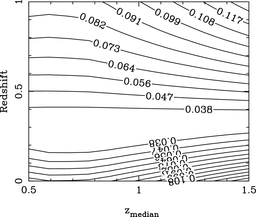
Figure 15: The uncertainty on $w(z)$, the dark energy equation of state measured at different redshifts, marginalized over all other parameters for gravitational lensing combined with 14-month Planck experiment, and its dependence on median redshift. The contours are lines of equal marginalized $w(z)$ error, the numbers on the lines being the marginal error on that line.

Figure 14 shows the expected accuracy of $w(z)=w_{0}+w_{a}z/(1+z)$ as a function of redshift for a 5-band, 10,000 square degree survey with median redshift $z_{m}=0.7$, combined with a 14-month Planck survey. The highest accuracy measurement occurs at $z=0.27$, where $w(z=0.27)=0.0298$. This low-redshift pivot redshift for the geometric test is due to its insensitivity to $w_{a}$.

Figure 15 shows how the error on $w(z)$ varies with both redshift, $z$, and with median redshift of the survey, $z_{m}$, for the same time-limited survey. It can be seen that the minimization in the error at $z\approx 0.7$ in Figure 11 is reproduced at the $z=0$ line (along the x-axis) of the plot, and Figure 14 is reproduced by considering the variation in the error along the $z_{m}=0.7$ line. It is clear that if one is concerned with optimizing a survey design to constrain the error on $w(z)$ at an optimal redshift then there is little sensitivity to the survey design. This is due to the effect of intersection, that is even though the lensing only error may be varying the intersection of the lensing ellipse with the Planck experiment ellipse does not vary considerably in width (characterized by the width of the inner contour) or orientation (characterized by the value of $z$ at which the error on $w(z)$ minimizes).

6.6.2 Figure of Merit

A useful ‘figure of merit’ (Linder, 2003; Linder, 2006; Dark Energy Task Force, DETF 2006) in dark energy predictions can be constrained by considering the smallest area of parameter space constrained by a given experiment. The dark energy equation of state can be written as:

$$w(a)=w_{i}+w_{a}(a_{i}-a)$$ (112)

where $w_{i}\equiv w(a_{i})$ and we have expanded around scale factor $a_{i}$. The error on $w(a)$ is:

$$\Delta w(a)^{2}=\Delta w_{i}^{2}+(a_{i}-a)^{2}\Delta w_{a}^{2}+2(a_{i}-a){\rm Cov}(w_{i},w_{a})$$ (113)

where ${\rm Cov}(w_{i},w_{a})$ is the covariance between $w_{i}$ an $w_{a}$ (equal to the corresponding inverse Fisher matrix element). By taking the derivative of this quantity the scale factor at which the error minimizes can be found

$$a_{{\rm min}}=a_{i}+\frac{{\rm Cov}(w_{i},w_{a})}{\Delta w_{a}^{2}}.$$ (114)

In the standard expansion in equation (6) $a_{1}=1$ and the above expression reduces to the equation for the pivot redshift. In this formalism the pivot redshift occurs when the covariance between the $w_{i}$ and $w_{a}$ is zero. This is equivalent to the pivot redshift in the formalism of equation (6). The ellipse at the pivot redshift is then the smallest ellipse constrained by a given experiment. Since this ellipse is de-correlated its area can be simply approximated by

$$\Delta w(a_{\rm pivot})*\Delta w_{a}.$$ (115)

This is the figure of merit used to quantify the performance of any given experiment: the smaller the figure of merit the tighter the constraints on the equation of state of dark energy will be over a larger redshift range. Broadly it can visualized by comparing Figure 15 and Figure 16, the figure of merit is minimized where the lowest contour in Figure 15 is widest, this can be seen in Figure 16. It can be seen that the optimal experiment when considering the figure of merit is at a median redshift of $z_{m}=0.7$ for $5$ bands. The figure of merit is shown for all considered experiments in Table 4.

Figure 16: The figure of merit as a function of median redshift, $z_{m}$, for a time-limited survey, assuming a 14-month Planck prior. The survey area is $A=10,000(z_{m}/0.7)^{-4}$ square degrees. The solid line is for $5$-band photometric redshift survey, the dashed line for $9$-band and the dot-dashed line for $17$-band.

7 Parameter Forecasts

Having found the optimal survey strategy to measure the dark energy equation of state for a given experiment, we can now investigate the constraints on the full parameter space. Throughout we shall assume a 10,000 square degree 5-band photometric redshift weak lensing survey with a median redshift of $z_{m}=0.7$ ($r=23.8$).

In this Section we shall discuss dark energy parameter constraints from geometric lensing alone (Section 7.1), combined with the WMAP 4-year and 14-month Planck experiments (Section 7.2), and combined with a WFMOS BAO experiment and SNAP SNIa experiment in Section 7.2 and 7.3. A table of the different surveys we have considered, and the predicted marginal errors on the dark energy parameters, is presented in Table 4.

Using the full Fisher matrix formalism for parameters in a consistent cosmological model we can estimate the accuracy on a set of cosmological parameters for a given experiment, taking into account marginalization over all other parameters. The details of the Fisher analysis are discussed in Section 6.1. The 11-parameter cosmological parameter set we shall use is ($\Omega_{m}$, $\Omega_{v}$, $h$, $\sigma_{8}$, $\Omega_{b}$, $w_{0}$, $w_{a}$, $n_{s}$, $\tau$, $\alpha_{n}$, $r=T/S$), with default values (0.27, 0.73, 0.71, 0.8, 0.04, -1.0,0.0, 1.0, 0.09, 0.0, 0.01). We shall compare and combine analysis with the results from a weak shear spectral analysis (e.g. Heavens et al., 2006) elsewhere.

7.1 Parameter forecasts for the geometric lensing test alone

On its own, the geometric test constrains a sheet in the likelihood space of ($w_{0}$, $w_{a}$, $\Omega_{v}$, $\Omega_{m}$). Figure 17 shows this plane in the 3-space of ($w_{0}$, $\Omega_{v}$, $\Omega_{m}$), having marginalized over $w_{a}$ (light grey plane). The surface here encloses the 3-parameter, 1-$\sigma$ likelihood surface. The equation of this plane in the full 4-parameter space is

$$X=0.64w_{0}-0.31w_{a}-0.35\Omega_{v}-0.67\Omega_{m}.$$ (116)

For model parameters of $w_{0}=-1$, $w_{a}=0$, $\Omega_{m}=0.27$, and $\Omega_{v}=0.73$ this can be evaluated to give

$$X=-1.08,$$ (117)

which can be measured with an expected accuracy of

$$\Delta X=0.031.$$ (118)

If we fix $w_{0}=-1$ and $w_{a}=0$, we can see that the geometric test constrains the degenerate line $\Omega_{v}+1.91\Omega_{m}=1.26$. This can be compared with the CMB constraint on the density parameter plane of $\Omega_{v}+\Omega_{m}=1$.

We can project this onto a 2-parameter space, marginalizing over all other parameters. Figure 18 show the 2-parameter, 1-$\sigma$ (68.3% confidence) likelihood contours for the parameter space of $\Omega_{v}$, $\Omega_{m}$, $w_{0}$ and $w_{a}$. The lightest grey solid block is the constraint on parameters from the lensing geometric method only. Here again we see the large degeneracies between the geometric parameters. In particular it is again clear that the geometric test is very insensitive to $w_{a}$ (see Section 2.3). The 1-parameter, 1-$\sigma$ marginalized parameter uncertainties can be found by projecting these contours onto each axis and dividing by $2.3$. These are presented in Table 4.

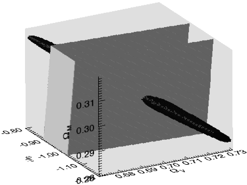
Figure 17: 3D parameter space for a 10,000 square degree lensing survey to a median redshift of $z_{m}=0.7$ with 14-month Planck experiment, with no dark energy evolution. The volumes bounded by light and dark grey which represent the 1-$\sigma$ parameter estimations for weak lensing and a 14-month Planck experiment respectively.

7.2 Comparing and combining the geometric lensing and the CMB

To lift the degeneracies in the geometric test we can combine our predictions with results expected from the CMB. Here we consider combining with the expected results from the 4-year WMAP experiment. Below we shall compare with the results expected from a 14-month experiment with the Planck Surveyor.

7.2.1 Combining with WMAP

The parameter forecasts for a $4$-year WMAP survey are compared and combined with the geometric test, allowing for spatial curvature, in Figure 18. The lightest grey ellipses are the geometric test alone, the darkest ellipses are the marginalized parameter forecasts for WMAP, while the central white ellipses, show the combined likelihood contours for the combined CMB and geometric methods. We have suppressed the amplitude of density perturbations parameterized by $\sigma_{8}$, the Hubble parameter $h$, the optical depth $\tau$, and the tensor-to-scalar ratio $r$, which are also estimated by the CMB. We shall consider these parameters in Section 7.2.2.

Figure 18 illustrates the poor sensitivity of the CMB to $w_{0}$ and $w_{a}$, but constrains the curvature of the model by the combination $\Omega_{m}+\Omega_{v}$. The response of the CMB to dark energy comes mainly from the Integrated Sachs-Wolf (ISW) effect. Combining the geometric lensing test and the CMB, we find the orthogonality of the two methods reduces the error on the dark energy parameters from $\Delta w_{0}({\rm WMAP})=1.268$, $\Delta w_{a}({\rm WMAP)}=2.225$ to $\Delta w_{0}({\rm WMAP+GL})=0.089$ and $\Delta w_{a}({\rm WMAP+GL})=0.714$. There is also marginal improvement in $\Delta\Omega_{m}$ and $\Delta\Omega_{v}$. The main improvement to the lensing analysis is the WMAP constraint on the curvature of the Universe in the $\Omega_{m}$, $\Omega_{v}$ parameter plane. To get a clearer picture of the orthogonality of the CMB 4-year WMAP and lensing geometric test results, we plot a 3-D view of the one-parameter, 1-$\sigma$ parameter surfaces in Figure 17. This shows the $w_{0}$, $\Omega_{m}$, $\Omega_{v}$ parameter surfaces, marginalized over all other parameters, including $w_{a}$.

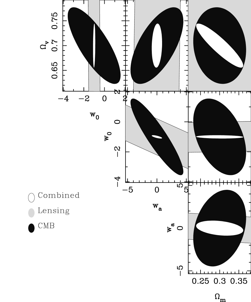
Figure 18: Two-parameter, 1-$\sigma$ (68.3% confidence) likelihood contours for geometric parameters for a 10,000 square degree lensing survey geometric analysis to a median depth $z_{m}=0.7$, compared and combined with the expected 4-year WMAP results.

7.2.2 Combining with Planck Surveyor

We can compare the information in Figure 18 from a 4-year WMAP experiment with that of a $14$-month Planck Surveyor experiment, shown in Figure 19. While the Planck error ellipses (darkest grey) are considerably smaller than those of the 4-year WMAP, the degeneracy between $w_{0}$ and $w_{a}$ remains. On its own Planck can measure $w_{0}$ to an accuracy of $\Delta w_{0}=0.502$ and on $w_{a}$ to an accuracy of $\Delta w_{a}=1.86$, with the main source of information from the Integrated Sachs-Wolfe (ISW) effect. Again the curvature of the model is well constrained by the CMB. Combining Planck with the geometric lensing test reduced the dark energy parameter uncertainties to $\Delta w_{0}=0.075$ and $\Delta w_{a}=0.326$, a factor of $\sim 7$ improvement in the measurement of $w_{0}$ over Planck alone.

The effect of the geometric tests constraints within an 11-dimensional parameter space can be seen in Figure 20. All other parameters are marginalized over. Even though the geometric test does not place any direct constraint on the non-geometric parameters, we note that there is improvement in the normalization of matter perturbations, $\sigma_{8}$. This arises because $\sigma_{8}$, measured from the CMB is dependent on the parameters. Hu & Jain (2004) show the dependence of $\sigma_{8}$ on other cosmological parameters, and in particular a constant value of $w$. In calculating the value of $\sigma_{8}$ using dark energy dependent growth factors they find that the value of $\sigma_{8}$ depends on a combination of dark energy parameters, they find an analytic expression in the special case of a flat Universe with constant $w$. These general arguments can be generalized to $w_{0}$ and $w_{a}$ using the growth factors given in Linder (Linder, 2003). An alternative parameter would be to use the horizon-scale amplitude of matter perturbations, $\delta_{\xi}$, which is an independent parameter. We have chosen to use $\sigma_{8}$ to compare with other analysis. The improvement on CMB parameters are summarized in Table 3.

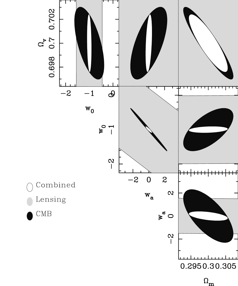
Figure 19: Two-parameter, 1-$\sigma$ (68.3% confidence) likelihood contours for geometric parameters for a 10,000 square degree lensing survey to a median depth $z_{m}=0.7$, with a 14-month Planck experiment. Note the change in the scale of the axes from Figure 18, from hereon the remaining Figures will uses the scale introduced in this Figure.

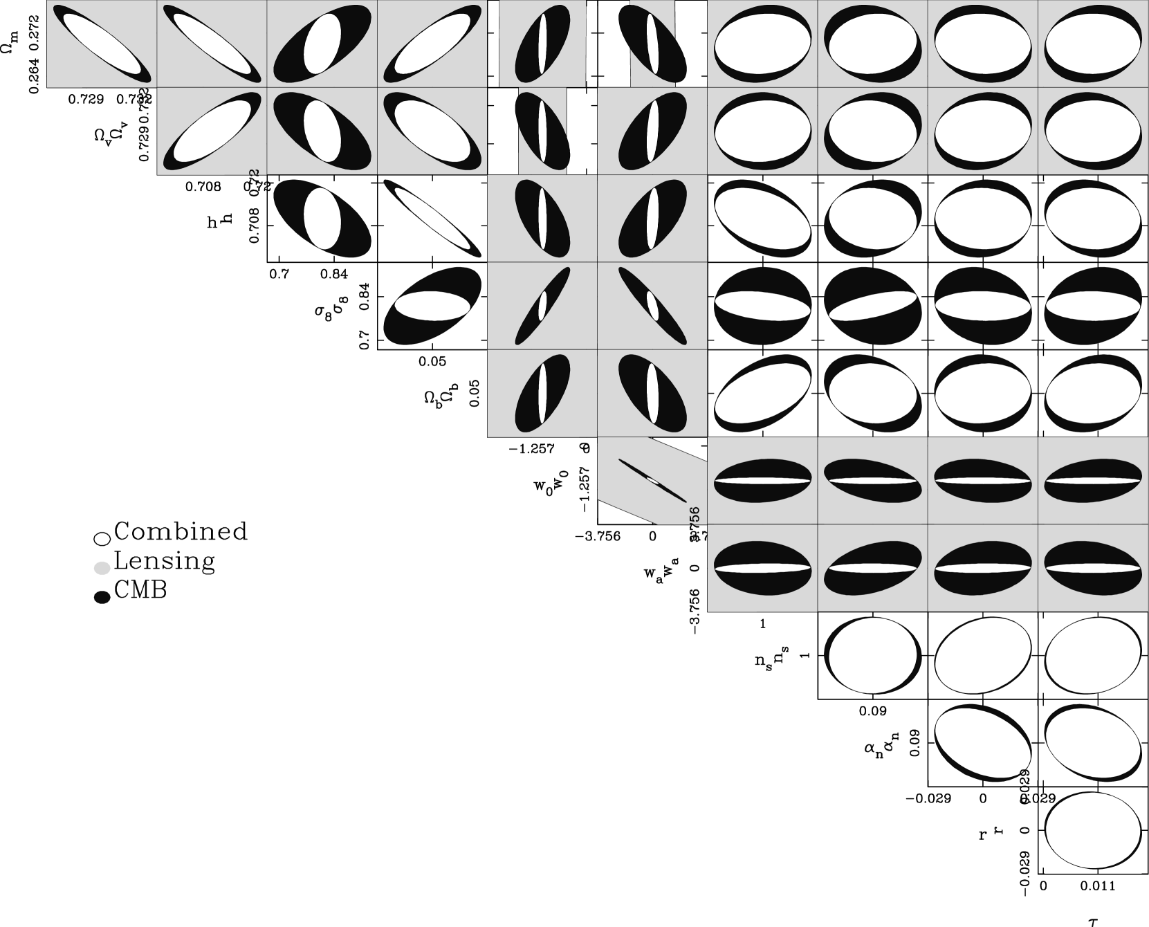
Figure 20: The two parameter 1-$\sigma$ (68.3% confidence) geometric constraints for a 10,000 square degree lensing survey to a median depth $z_{m}=0.7$, with a 14-month Planck experiment in the 11-dimensional parameter space ($\Omega_{m}$, $\Omega_{v}$, $h$, $\sigma_{8}$, $\Omega_{b}$, $w_{0}$, $w_{a}$, $n_{s}$, $\tau$, $\alpha_{n}$, $r$). Other parameters for the CMB calculation are marginalized over.

Parameter	Planck only	Combined
$\Omega_{m}$	$0.0058$	$0.0042$
$\Omega_{v}$	$0.0024$	$0.0020$
h	$0.0088$	$0.0070$
$\sigma_{8}$	$0.1002$	$0.0383$
$\Omega_{b}$	$0.0011$	$0.0008$
$w_{0}$	$0.5015$	$0.0751$
$w_{a}$	$1.8618$	$0.3256$
$n_{s}$	$0.0034$	$0.0034$
$\alpha_{n}$	$0.0062$	$0.0056$
$\tau$	$0.0208$	$0.0204$
$r$	$0.0079$	$0.0077$

Table 3: Improvements on CMB Planck one parameter 1-$\sigma$, constraints by adding the geometric test from a 10,000 square degree lensing survey to a median depth of $z_{m}=0.7$.

7.2.3 Comparing and combining lensing with CMB, BAO and SNIa experiments

Figure 21 shows comparisons between the geometric lensing, CMB, SNIa and BAO experiments for the geometric parameter set $(\Omega_{m},\Omega_{v},w_{0},w_{a})$. The broad, second lightest grey ellipses are for a SNAP-like SNIa experiment, the closed darker ellipses are for a WFMOS-like BAO experiment, the lightest grey is for the lensing geometric test, while the darkest ellipse is for a 14-month Planck CMB experiment. The small white ellipse at the centre is the combined uncertainty. We have scaled the axes so that the full parameter degeneracies can be seen. It is clear that allowing for spatial curvature and evolution of the dark energy opens up large degeneracies in many of the experiments. Because of the large-data set and sensitivity of the CMB to parameters, the CMB provides the strongest constraints alone. In particular we can see very similar degeneracies between experiments in the $(\Omega_{v},w_{0})$ plane, while there is some orthogonality between experiments in the $(w_{0},w_{a})$ plane. Combining experiments improves the constraints on all of the parameters. In particular, allowing for spatial curvature we find $\Delta w_{0}=0.043$, and $\Delta w_{a}=0.108$. We shall study the combination of experiments in more detail in Section 7.3.

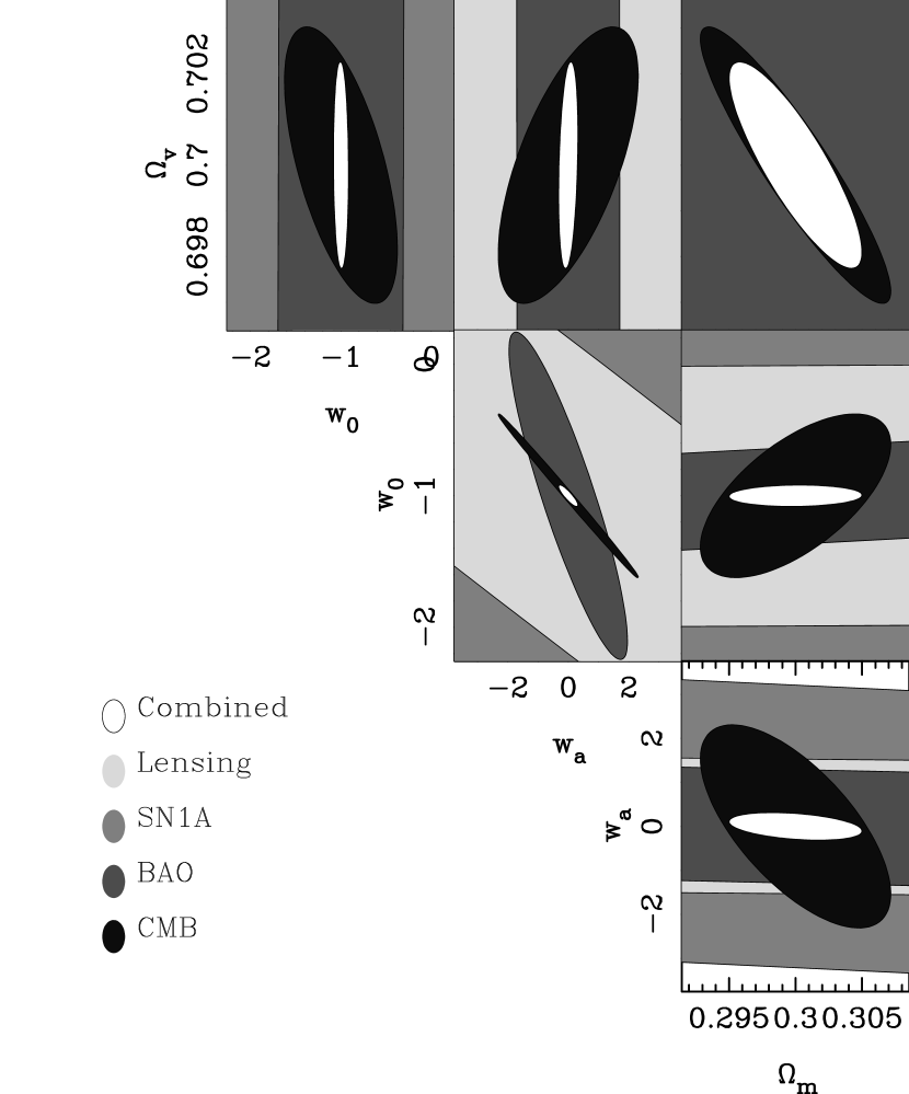
Figure 21: Two-parameter, 1-$\sigma$ (68.3% confidence) likelihood contours for geometric parameters for a 10,000 square degree lensing survey to a median depth of $z_{m}=0.7$, combined with a 14-month Planck experiment, a WFMOS BAO experiment and a SNAP SNIa experiment. 1-parameter marginalized results are tabulated in Table 4.

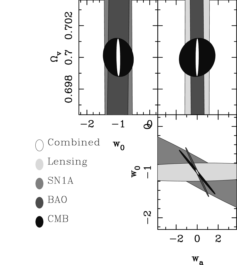
Figure 22: Two-parameter, 1-$\sigma$ (68.3% confidence) likelihood contours for geometric parameters for a 10,000 square degree lensing survey to a median depth of $z_{m}=0.7$, with a 14-month Planck experiment, a WFMOS BAO experiment and a SNAP SNIa experiment, assuming spatial flatness with $\Omega_{m}+\Omega_{v}=1$.

In Figure 22 we show the same set of parameters, but this time assuming spatial flatness. Again many of the largest degeneracies in each of the experiments remain. We also see clearly the insensitivity of the geometric lensing to $w_{a}$, rendering it nicely orthogonal to the other experiments. Also note that the two geometric methods considered, the geometric test and the supernovae test constrain similar regions in the ($w_{0}$, $w_{a}$) plane. Comparing Figure 21 and Figure 22 it is clear that the assumption of flatness improves the marginal errors of the lensing, BAO and SNIa significantly, however since the CMB experiment constrain flatness to a high degree the overall combined constraints are broadly the same. This highlights the danger of assuming flatness, given that the marginal errors without a CMB experiment are drastically altered by this assumption. Given that some dark energy models involve variations to the Friedmann equation in non-flat geometries it is prudent to marginalize over spatially curved models.

To illustrate further the orthogonality of the constraints from lensing, the CMB, BAO and SNIa, Figure 23 shows a 3-dimensional plot of the likelihood contours in the $(\Omega_{v},w_{0},w_{a})$ parameter space, marginalizing over all other parameters. We have plotted the 1-parameter, 1-sigma contours for clarity.

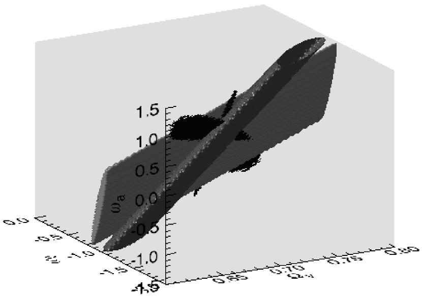
Figure 23: Likelihood contours in the 3-dimensional $\Omega_{v}$, $w_{0}$, $w_{a}$ parameter space for geometric parameters for a 10,000 square degree lensing survey to a median depth of $z_{m}=0.7$, with a 14-month Planck experiment, a WFMOS BAO experiment and a SNAP SNIa experiment, assuming spatial flatness, $\Omega_{m}+\Omega_{v}=1$. 1-parameter, 1-sigma contours are used for clarity.

7.3 Synergy of dark energy experiments

It is interesting to compare the results of each of the dark energy experiments under the same conditions. In Figure 24 we show the dark energy equation of state parameters $(w_{0},w_{a})$, marginalized over all other parameters including spatial curvature for each experiment in combination.

Of all of the individual experiments considered the Planck CMB experiment on its own provides the strongest constraint on the ($w_{0},w_{a}$) plane, with the majority of the signal coming from the low-redshift ISW effect. However the marginalized uncertainties are still $\Delta w_{0}=0.502$ and $\Delta w_{a}=1.86$. A SNAP-like SNIa experiment on its own provides poor constraints in the $w_{0}$, $w_{a}$ plane, due to the large degeneracy in $\Omega_{m}$ and $\Omega_{v}$ in models allowing curvature. This can be seen by comparing with Figure 22, but note that of the experiments considered, the supernova estimates are the only ones which include terms for extra systematic effects. Removing the extra systematic terms from the supernova estimates improves the constraints, when combined with a Planck CMB prior, by a factor of approximately $1.5$ to $\Delta w_{0}=0.094$ and $\Delta w_{a}=0.318$. A WFMOS-like BAO experiment provides a narrow, but highly degenerate ellipse in the $(w_{0},w_{a})$ plane. This is due to the BAO experiment mainly constraining $w(z)$ at the redshift of the nearest redshift bin (in this case $z=1.0$). Interestingly the BAO degeneracy is in a similar direction to the CMB degeneracy, presumably because a similar geometric effect is being measured. Finally, the geometric lensing again has a large degeneracy in this plane, but one which is different from the other experiments.

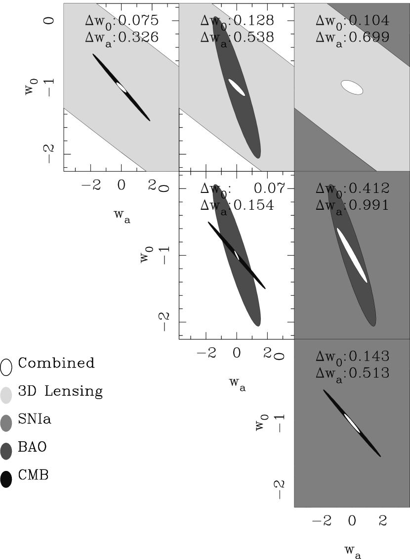
Figure 24: The combined marginal $w_{0}$, $w_{a}$ constraints for two pairs of experiments. The experiments are a darkCAM lensing experiment and a CMB 14-month Planck experiment, a BAO WFMOS experiment and a SNIa SNAP experiment. Note that only the SNIa analysis contains terms for systematic effects. See Section 4.9 for details.

The combination of pairs of experiments is very interesting. The combination of the geometric lensing and CMB puts very strong constraints on the dark energy equation of state and its evolution, reducing the uncertainty to $\Delta w_{0}=0.075$ and $\Delta w_{a}=0.326$. Geometric lensing and SNIa yields $\Delta w_{0}=0.104$ and $\Delta w_{a}=0.699$ while geometric lensing and BAO yields $\Delta w_{0}=0.128$ and $\Delta w_{a}=0.538$. This provides us with three cross-checks with similar accuracy. Looking at the dependency of each method, we see that both the geometric lensing, BAO and SNIa are all dependent on the geometry of the Universe, and so should give the same result, assuming that the $w_{0},w_{a}$ parameterization is valid. The CMB combines geometry with evolution of the potential field, particularly in the ISW effect.

Looking at the other possible combinations without lensing we see there is a similar sensitivity to dark energy. We have already pointed out the degeneracy between the BAO and CMB constraints, and so their combination only marginally improves on the CMB alone. A similar result is found for combining CMB and SNIa. Finally BAO and SNIa provides an uncertainly similar to CMB alone.

From this study, we conclude that the best pair combinations come from combining geometric lensing with any of CMB, BAO or SNIa experiments, with $\Delta w_{0}\sim 0.10$ and $\Delta w_{a}\sim 0.50$, and also the BAO and CMB combination. Multiple combinations will also allow a degree of cross-checking for consistency. Other combinations are a factor of up to 5 times poorer due to similar degeneracies between $w_{0}$ and $w_{a}$.

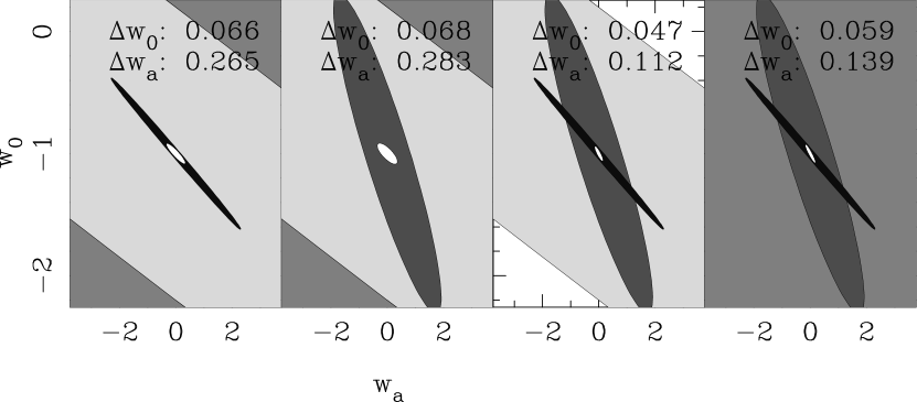
Figure 25: The marginal $w_{0}$, $w_{a}$ constraints for a combination of any three of the dark energy experiments. A darkCAM lensing experiment, CMB 14-month Planck experiment, BAO WFMOS experiment and a SNIa SNAP experiment.

Combining three experiments, in Figure 25 we again see that strongest measurement of $(w_{0},w_{a})$ comes from combining the geometric lensing analysis with the CMB and BAO experiments with the uncertainty on $w_{0}$ and $w_{a}$ pushed down to $\Delta w_{0}=0.047$ and $\Delta w_{a}=0.112$. Adding the SNIa results to this makes no a small difference (see Figure 26, but again recall that the SNIa is the only estimate to contain systematic effects). Again the all the three experiment combinations all provide complimentary constraints in the ($w_{0}$, $w_{a}$) plane.

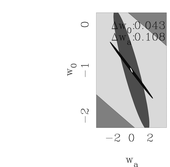
Figure 26: The marginal $w_{0}$, $w_{a}$ constraints for a darkCAM lensing experiment and a CMB 14-month Planck experiment, a BAO WFMOS experiment and a SNIa SNAP experiment.

Survey	Area sqdeg	$\rm z_{{\rm median}}$	$N_{\rm Bands}$	$\Delta w_{0}$	$\Delta w_{a}$	${\rm z_{{\rm pivot}}}$	$\Delta w({\rm z_{{\rm pivot}}})$	$\Delta w({\rm z_{{\rm pivot}}})\Delta w_{a}$
Lensing
darkCAM	$10000$	$0.7$	$5$	$5.546$	$31.132$	$0.21$	$0.972$	$30.2471$
darkCAM + Planck	$10000$	$0.7$	$5$	$0.075$	$0.326$	$0.27$	$0.030$	$0.0097$
darkCAM + BAO darkCAM	$10000$	$0.7$	$5$	$0.459$	$1.668$	$0.01$	$0.419$	$0.6984$
darkCAM, $9$ bands + Planck	$10000$	$0.7$	$9$	$0.071$	$0.311$	$0.26$	$0.029$	$0.0089$
SNAP Lensing + SNIa + Planck	$1000$	$1.38$	$9$	$0.073$	$0.293$	$0.31$	$0.024$	$0.0071$
All-Sky Space + Planck	$40000$	$1.00$	$9$	$0.023$	$0.146$	$0.16$	$0.012$	$0.0017$
darkCAM+Planck+BAO+SNIa	$10000$	$0.7$	$5$	$0.043$	$0.108$	$0.58$	$0.018$	$0.0019$
VST-KIDS+WMAP4	$1400$	$0.6$	$5$	$0.227$	$0.888$	$0.19$	$0.176$	$0.1562$
CFHTLS(Wide)+WMAP4	$170$	$1.17$	$5$	$0.282$	$1.014$	$0.29$	$0.1663$	$0.1687$
CMB
4-year WMAP				$2.060$	$3.612$	$1.18$	$0.758$	$2.7379$
14-Month Planck				$0.501$	$1.873$	$0.367$	$0.035$	$0.0655$
BAO
BAO WFMOS+Planck	$2000$	$1.0$		$0.070$	$0.154$	$0.78$	$0.019$	$0.0029$
SNIa
SNIa SNAP+Planck				$0.142$	$0.513$	$0.37$	$0.028$	$0.0144$

Table 4: The table gives experimental parameters and marginalized cosmological parameter error forecasts for various surveys.

7.4 Complementary Figures of Merit and Pivot Redshifts

The figure of merit and pivot redshift information can be represented as in Figure 27 so that both values can be seen simultaneously. The Figure shows a number of broad characteristics. As more experiments are added in combination both the pivot redshift converges to one mean value and the figure of merit decreases. The geometric test constraint forces the pivot redshift to lower values due to its unique degeneracy whilst the BAO constraint forces the pivot redshift to higher values. It is also evident that the CMB constraint is not necessary for a low figure of merit (for example LBS). This Figure also shows how different combinations of surveys can probe dark energy at significantly different redshifts. For example the BC and LSC combinations both have a similar figure of merit with the BC combination $z_{\rm pivot}=0.76$ and the LB combination $z_{\rm pivot}=0.28$.

Figure 27: The figure of merit and pivot redshift for various experimental combinations. The combinations are labeled as L=Lensing, B=BAO, S=SNIa, C=CMB. Combinations of letters represent combinations of experiments.

7.5 The effect of changing the fiducial dark energy model

The assumed fiducial cosmology has so far been a $\Lambda$CDM cosmology in which any derivatives in the Fisher matrix calculations have been about $w_{0}=-1.0$ and $w_{a}=0.0$ for the equation of state parameters. The effect of altering this assumption is investigated here. We consider two alternative extremes which are just allowable by present constraints, dark energy models: a SUGRA (Super Gravity) model proposed by Weller & Albrecht (2002) represented by $w_{0}=-0.8$ and $w_{a}=+0.3$; and a phantom model proposed by Caldwell et al. (2003) with $w_{0}=-1.2$ and $w_{a}=-0.3$. To test the effect of changing our default dark energy model we re-run our Fisher analysis.

Aswell as changing the point in parameter space about which the signal ratio is expanded in the Fisher matrix calculations the assumed fiducial dark energy model also affects the SIS to NFW scaling as a function of redshift and mass, as shown in Figure 6. It also affects the number density distribution of haloes as a function of redshift and mass given by equation (48), when extending to arbitrary dark energy models we exchange the growth factor in equation (54) to the one given in Linder & Jenkins (2003).

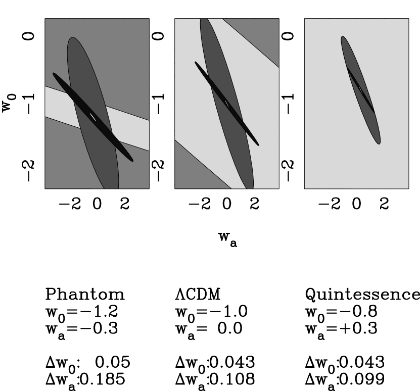
Figure 28: The dependence of the marginal error on $w_{0}$ the assumed dark energy model, for a 10,000 square degree survey to a median depth $z=0.7$, with a 14-year Planck prior, a BAO WFMOS prior and a SNIa SNAP prior. The errors quoted are marginal over all parameters.

The effects of changing the default dark energy model are shown in Figure 28, where we plot the $(w_{0},w_{a})$ plane, fully marginalizing over all other parameters. The marginal errors for each experiment, and its degeneracy in parameter space does indeed depend on the dark energy model. But the combined marginal errors do not significantly change. The main difference is manifest in the error on $w_{a}$ which increases for all methods as its value becomes more negative. This is simply due to the fact that a negative $w_{a}$ represents a dark energy scenario in which the dark energy density was less in the past (increasing in the future); so that the effect of dark energy on the expansion rate on observed galaxies (in the past) is less in these scenarios (and similarly the opposite effect for a positive $w_{a}$).

8 Additional Systematic Effects for Lensing

In this Section we consider come potential systematic effects for weak lensing. To realize a $\sim 1\%$ measurement of $w_{0}$ and $w_{a}$ from shear ratios not only do we need a large enough survey, but we must also be able to control systematics in a weak lensing survey to a high level. This will require controlling the systematics in the measurement of lens shear to $\Delta\gamma\sim 10^{-5}$.

8.1 Image Shear Analysis

The current generation of lensing surveys, with telescopes not specifically designed for lensing, induce $10\%$ distortions, which can be corrected down to a net systematic of $0.01\%$ ($\Delta\gamma\sim 10^{-4}$; Heymans et al., 2005). There has been extensive work into methods that can both diagnose and remove systematic errors from both intrinsic galaxy alignments (Hirata et al., 2004) and shear calibration errors. Mandelbaum et al. (2005) use a geometric test to diagnose systematic errors in the Sloan Digital Sky Survey (SDSS).

8.2 Strong Lensing Effects

There is a systematic effect in the strong lensing régime, where the reduced shear $e_{i}$, defined as

$$e_{i}=\frac{\gamma_{i}}{1-\kappa_{i}}$$ (119)

is measured from galaxy ellipticities. The ratio $R_{ij}$ now becomes

$$R_{ij}=\frac{e_{i}}{e_{j}}=\frac{\gamma_{i}(1-\kappa_{j})}{\gamma_{j}(1-\kappa_{i})}$$ (120)

which, for the mildly non-linear lensing régime can be approximated as

$$R_{ij}\approx\frac{\gamma_{i}}{\gamma_{j}}(1+\kappa_{i}-\kappa_{j})$$ (121)

Furthermore for a SIS $\kappa\approx\gamma$. This was numerically tested, using observable clusters, and the amplitude of the correction was found to be $\rm{max}(\kappa_{i}-\kappa_{j})\sim 0.15$ and $\rm{mean}(\kappa_{i}-\kappa_{j})\sim 1.5\times 10^{-3}$. This numerical analysis implicitly assumes a radius of $1$ arcmin from equation 38, which is relatively narrow: tangential shear can be measured out to radii of at least $200$ arcseconds see Gray et al. 2004. The largest source of this systematic error will be from the largest clusters, those producing the largest convergence, and as shown in Section 5 the majority of the $w_{0}$ signal comes from clusters of intermediate mass for which we would expect this systematic to be smaller.

Alternatively, one can construct a statistic which eliminates the mass-dependence of $\gamma/(1-\kappa)$, such as the three-point statistic suggested by Gautret, Fort & Mellier (2000). This could be applied in the strong-lensing régime, again independent of the lens strength, and combined with the two-point geometric ratio test in the weaker lensing régime. We shall investigate this elsewhere.

8.3 Cluster Substructure

A further expected systematic is that arising from cluster sub-structure, which we assume is averaged over. The effect of including sub-structure can only increase the signal; as long as the mass map of a cluster can be accurately measured the expected tangential shear signal can be modelled. One promising avenue which may yield information on sub-structure is flexion (see Bacon et al., 2005). In the low signal-to-noise régime (low galaxy number counts) in which a mass model may have to be assumed for a cosmological signal to be extracted then this systematic source of error will become important and the mass model will need to be accurately reproduced. However, in the high signal-to-noise régime where the number of available galaxies is such that ratio of the shears from the data can simply be taken this systematic source of error will not affect the analysis.

8.4 The effect of photometric redshift outliers

In any weak lensing photometric redshift survey there will be a sample of imaged galaxies that will not have photometric redshifts assigned. There will be several classes of objects, for some of which determining a photometric redshift will be difficult. We test the effect of such ‘outliers’ here by assuming a population within the survey $p2$ that have photometric redshifts $\sigma^{p2}_{z}(z)=0.5$, that is they have practically no redshift information.

There are two ways in which such a population can be used, either they are included in the sample of galaxies used somehow, or they are discarded. If they are used then the galaxies can be treated as a seperate population, with $\sigma^{p2}_{z}(z)=0.5$ and $n^{p2}=(1-A^{p2})n_{0}$ where $A^{p2}$ is the fraction of outliers in the total population, analysed independently and the constraints from the outliers added to the constraints from galaxies with good redshifts. Or, the effective redshift error distribution at a particular redshift $z$ can be modelled by the sum of two Gaussian distributions, with errors $\sigma^{p1}_{z}(z)$ and $\sigma^{p2}_{z}(z)$, the relative amplitudes of the Gaussians constrained so that $A^{p1}+A^{p2}=1$. Such a sum of Gaussians can be accurately modelled as an effective Gaussian, see Blake & Bridle (2005), with an effective width $\sigma_{eff}=\sqrt{A^{p1}[\sigma^{p1}_{z}(z)]^{2}+A^{p2}[\sigma^{p2}_{z}(z)]^{2}}$. We investigated varying the relative amplitudes of two Gaussians with $\sigma^{p1}_{z}(z)=\sigma_{z}(z)$, the original photometric redshift error from equation (57) and a second with $\sigma^{p2}_{z}(z)=0.5$.

Figure 29 shows the effect of varying the fraction of total population in oultiers, combined with a 14-month Planck prior, the solid line shows the constraints from treating the outliers as a seperate population analysed seperately, the dot-dashed line includes the outliers into a degraded population using an effective Gaussian. The second possibility, that of discarding the outlying sample, is investigated by simply reducing the surface number density by $n_{0}\rightarrow(1-A^{p2})n_{0}$, this is also shown in Figure 29 as the dashed line.

Figure 29: The dependence of the marginal error on $w_{0}$ on the amplitude of outliers with a $\sigma^{p2}_{z}(z)=0.5$ for a 10,000 square degree survey to a median depth $z=0.7$, with a 14-year Planck prior. The solid line combines the outliers constraint with the galaxies with good photometric redshift errors by adding the constraints. The dot-dashed line shows the effect of combining the outliers with the rest of the population using an effective Gaussian. The dashed line discards the outlying sample of galaxies.

All the methods for dealing with the outliers result in an increase in the marginal error on $w_{0}$. As expected using all the galaxies and treating the outliers as a seperate population has the smallest effect on the marginal error, by using the outliers the marginal error is less than when they discarded. The effective Gaussian method has the effect of decreasing the number of redshift bins in the survey that can be used while retaining the surface number density, thus decreasing the signal. By discarding the outliers the number of redshift bins is retained while the surface number density is uniformly degraded. This shows that the signal is more dependent on the number of redshift bins, than the number density and that the strategy for dealing with outliers will be an important issue in future surveys.

8.5 CMB Lensing

When combining the shear ratio analysis with CMB measurements we have assumed that the weak lensing of the CMB by large scale structure and galaxy clusters can effectively be ignored. Since the shear ratios do not contain any information about structure, there can be no correlation due to this. There may, however, be some correlation between lensing of the CMB and the noise term in the shear ratio method. We shall explore this elsewhere.

9 Conclusions

In this paper we have set out a new method for the analysis of the geometric shear ratio test for measuring the dark energy equation of state, based on the measurement of shear ratios around individual galaxy groups and clusters. The shear ratio test is insensitive to the growth of structure, but sensitive to the geometry of the Universe, via the matter and dark energy density and the dark energy equation of state. This approach allows one to apply the method to individual objects, rather than requiring the measurement of some other statistic such as the galaxy-shear cross-correlation function which may be noisy for small data-sets. The down-side is that the method is now contaminated by structure along the line of sight, which can be overcome by using many independent lines of sight.

Of the parameters which govern the geometry of the Universe, or more properly the photon distance-redshift relation, the shear ratio is most sensitive to a constant dark energy equation of state, $w_{0}$, and very insensitive to evolution, parameterized here by $w_{a}$. This can be understood as due to the shear ratios being sensitive only to the change in shape of the shear signal as a function of redshift. As $w_{a}$ parameterizes the high-redshift effect of the dark energy equation of state, its effects are “renormalized” away. This behavior is very different to other probes of dark energy, and so helps to break parameter degeneracies when combined with other probes.

It must be emphasised that the Fisher matrix framework used in this paper may result in overly optimistic constraints. Since the errors are calculated by expanding about a fiducial point in parameter space any higher order effects that may change the shape of the likelihood surface cannot be taken into account. The effect of varying the fiducial dark energy model, in Section 7.5, demonstrates that the errors are sensitive to the choice of the fiducial model. A concrete example of higher order likelihood effects can be seen in a 3D cosmic shear analysis by comparing Fisher matrix calculations of the ($\sigma_{8}$, $\Omega_{m}$) plane (for example in Heavens et al., 2006) (predicting an ellipse) with the measured constraints from data (for example Kitching et al., 2006) which measure an extended curved constraint. These effects can be investigated by large simulations or by a Monte-Carlo type exploration of the likelihood surface, we leave such investigations for future work.

To account for many of the sources of uncertainty in the method, we have developed a halo decomposition analysis of the lensing dark matter distribution to model the signal from dark matter haloes over a range of mass scales and redshifts. We have also included the effects of shot-noise due to the random intrinsic orientation of each galaxy, photometric redshift errors and the contribution of large-scale structure lensing to the error budget. We have also investigated in detail a model for the photometric redshift error, based on studies of the COMBO-17 data-set, as a function of redshift, number of imaging bands and limiting magnitude. The effect of a bias in the calibration and distribution of photometric redshifts with spectroscopic redshifts is also studied, and we find that we require some $10^{4}$ galaxies with spectroscopic redshifts to control calibration issues. The limitations of observing the shear signal from the ground and space are also discussed, and we argue that without adaptive optics ground-based lensing studies are seeing limited, suggesting that it will be difficult to use galaxies beyond $z=1.5$.

The halo decomposition analysis of the dark matter lenses has allowed us to probe the origin of the shear signal in different types of survey, taking a 4-metre telescope with a 2 square degree field of view as our default survey. These results can be scaled to any other telescope parameters.

For targeted observations, where the time-limitation translates into the number of clusters and groups one can observe to a given depth, we have shown that we only require around 60 of the largest clusters in a celestial hemisphere to constrain $w_{0}$ to around $\Delta w_{0}\sim 0.50$, marginalizing over all other parameters, including $w_{a}$, a factor of $3$ improvement on 4-year WMAP given a marginalization over $w_{a}$. To achieve a higher accuracy requires the imaging of an unfeasible number of haloes, and instead one should turn to a wide-field imaging and photometric redshift survey. We find for a 4-meter class telescope with a 2 degree field of view that with a 10,000 square degree, 5-band photometric redshift survey with median redshift $z_{m}=0.7$ ($r=23.8$), we can expect to reach an accuracy of $\Delta w_{0}\sim 0.07$, again marginalizing over all other parameters including $w_{a}$. Our results can be easily rescaled to other telescope types, and survey strategies.

The halo decomposition allows us to deduce where the main signal comes from in both the targeted and surveying modes. In both cases a significant fraction of the signal comes from the largest hundred clusters in each survey, reaching a sensitivity of $\Delta w_{0}\sim 0.5$, however the majority of the signal comes from the numerous ($\sim 10^{5-6}$) $M>10^{14}M_{\odot}$ haloes which can push the accuracy up to $\Delta w_{0}\sim 0.07$.

Having determined where the majority of the dark energy signal will come from in a geometric shear ratio test, we then investigate the optimization of such a survey, when combined with the expected results from the Planck Surveyor experiment. We find that for our fiducial telescope for a fixed-time survey, going shallower ($z_{m}<0.7$) over a wider area decreases the accuracy due to the drop in the number of available background sources and corresponding increase in shot-noise. Going deeper ($z_{m}>0.7$) over a smaller area increases the clustering noise, since we now have fewer clusters to average over.

We have also studied the effect of varying the number of imaging bands to increase or decrease the photometric accuracy. We find that when combined with Planck an increase from 5, 9 or 17 optical bands makes little difference to the optimal survey. The reason for this insensitivity to higher accuracy photometric redshifts is due to the integral nature of the lensing effect, and the weak effect when combined with another data-set. However decreasing the number of bands is expected to have a strong effect on the accuracy of the lensing survey as redshift information is lost. We discuss how our results can be scaled to other telescope classes and survey parameters.

The dark energy parameters $w_{0}$ and $w_{a}$ can be combined to give an uncertainty on $w(z)=w_{0}+w_{a}z/(1+z)$, at some optimal redshift. This combination helps distinguish where the survey is most sensitive to the dark energy equation of state. In the case of our optimal lensing survey this is at $z=0.27$ with $\Delta w(z=0.27)=0.0298$. Again, the reason for the low-redshift sensitivity to $w(z)$ is due to the insensitivity of the shear ratio test to $w_{a}$.

Having optimized the lensing survey for the geometric test in combination with the expected results from the CMB, we have investigated the effect on the full set of cosmological parameters for the CMB and lensing. The geometric test constrains a narrow sheet in the $(\Omega_{m},\Omega_{v},w_{0},w_{a})$ parameter-space, which is nicely orthogonal to the CMB parameter constraints. Here we show that the CMB mainly constrains the curvature of the model, while the geometric test constrains $w_{0}$, and the combination constrain $w_{a}$.

We have also compared and combined the geometric shear ratio test with the expected results from an Baryon Acoustic Oscillation (BAO) experiment, such as proposed for WFMOS, and a supernova Type Ia survey, such as that proposed for SNAP. Here we have put all of the surveys (lensing, CMB, BAO and SNIa) on an equal footing, using the same curved background cosmology and the same dark energy model parameterization. We find that the degeneracies in the geometric test, in particular the insensitivity to $w_{a}$, are nicely orthogonal to all these other probes. Combining the geometric test with the CMB, BAO or SNIa will yield accuracies of a $\Delta w_{0}\approx 0.10$ and $\Delta w_{a}\approx 0.5$, and can be compared for systematics. An optimal combination is a geometric lensing test, with the Planck CMB and WFMOS BAO experiment, yielding an expected accuracy of $\Delta w_{0}=0.047$ and $\Delta w_{a}=0.11$.

Finally we discuss some of the potential systematic effects which could affect the predicted accuracy of lensing.

In summary, the prospects of accurately measuring the dark energy equation of state and its evolution to high accuracy over the next decade are very good. The key to this is the gravitational lensing geometric shear ratio test, which, due to its orthogonal degeneracies, can be optimally combined with a large range of other dark energy probes, such as the CMB, BAO or SNIa. In addition, gravitational lensing can also be a probe via two-point analysis, either from correlation functions or power spectra in redshift-space (Heavens et al. 2006 and Castro et al. 2005). Just as with lensing of the CMB, since the shear ratio analysis does not contain any information on structure, we can expect there to be little correlation between the two methods, even for the same survey. However, the shear ratio covariance may be correlated with the shear power. We shall explore combining these methods elsewhere.

Appendix A: Covariance of tangential cosmic shear

The cosmic tangential shear covariance averaged over a circular aperture is given by

$$C^{\gamma_{t}\gamma_{t}}(\theta) = \frac{1}{A^{2}}\int d^{2}\!\theta\int\!d^{2}\theta^{\prime}\,\langle\gamma_{t}(\mbox{\boldmath$\theta$})\gamma_{t}(\mbox{\boldmath$\theta$}^{\prime})\rangle$$ (122)

$$= \frac{1}{A^{2}}\int\!d^{2}\theta\int\!d^{2}\theta^{\prime}\,\left(\langle\gamma_{1}(\mbox{\boldmath$\theta$})\gamma_{1}(\mbox{\boldmath$\theta$}^{\prime})\rangle\cos 2\varphi\cos 2\varphi^{\prime}+\langle\gamma_{2}(\mbox{\boldmath$\theta$})\gamma_{2}(\mbox{\boldmath$\theta$}^{\prime})\rangle\sin 2\varphi\sin 2\varphi^{\prime}\right)$$

$$= \frac{1}{A^{2}}\int\!d^{2}\theta\int\!d^{2}\theta^{\prime}\,\left[\int\!\frac{d^{2}\ell}{(2\pi)^{2}}\,C^{\kappa\kappa}_{\ell}(\cos^{2}2\varphi_{\ell}\cos 2\varphi\cos 2\varphi^{\prime}+\sin^{2}2\varphi_{\ell}\sin 2\varphi\sin 2\varphi^{\prime})e^{i\mbox{\boldmath$\ell$}.(\mbox{\boldmath$\theta$}-\mbox{\boldmath$\theta$}^{\prime})}\right]$$

$$= \int\!\frac{d^{2}\ell}{(2\pi)^{2}}\,C^{\kappa\kappa}_{\ell}\cos^{2}2\varphi_{\ell}\left(\frac{1}{A}\int\!d^{2}\theta e^{i\mbox{\boldmath$\ell$}.\mbox{\boldmath$\theta$}}\cos 2\varphi\right)^{2}$$

$$= \int_{0}^{\infty}\!\frac{\ell d\ell}{\pi}\,C^{\kappa\kappa}_{\ell}\left\{\frac{2[1-J_{0}(\ell\theta)]}{\ell^{2}\theta^{2}}-\frac{J_{1}(\ell\theta)}{\ell\theta}\right\}^{2}$$

where $\cos\varphi_{\ell}=\mbox{\boldmath$\hat{\ell}$}.\mbox{\boldmath$\hat{\theta}$}_{1}$ and $\mbox{\boldmath$\hat{\theta}$}_{1}$ is the unit vector along one axis.

Appendix B: Bias in assumed parameters

In this Appendix we show that for a Gaussian distributed likelihood function, the linear bias in a parameter, which we shall call $\delta\theta_{i}$, due to a bias in a fixed model parameter (i.e., one whose value we have assumed and is not being measured), which we shall call $\delta\psi_{j}$, is given by (e.g., Knox, Scoccimarro and Dodelson, 1998; Kim et al., 2004)

$$\delta\theta_{i}=-[F^{\theta\theta}]^{-1}_{ik}F^{\theta\psi}_{kj}\delta\psi_{j},$$ (123)

where $\mbox{\boldmath$F$}^{\theta\theta}$ is the parameter Fisher matrix defined as

$$F^{\theta\theta}_{ij}=\frac{1}{2}{\rm Tr}(C^{-1}\partial_{i}^{\theta}CC^{-1}\partial_{j}^{\theta}C+2\partial_{(i}^{\theta}\mu C^{-1}\partial_{j)}^{\theta}\mu^{T})$$ (124)

and $\mbox{\boldmath$F$}^{\theta\psi}$ is a column matrix (for one bias parameter) defined as

$$F^{\theta\psi}_{ij}=\frac{1}{2}{\rm Tr}(C^{-1}\partial_{i}^{\theta}CC^{-1}\partial_{j}^{\mu}C+\partial_{i}^{\theta}\mu C^{-1}\partial_{j}^{\psi}\mu^{T}+\partial_{i}^{\psi}\mu C^{-1}\partial_{j}^{\theta}\mu^{T})$$ (125)

which we will refer to as a pseudo-Fisher matrix between measured and assumed parameters.

We begin with a Likelihood function, $\ln L(\mbox{\boldmath$\theta$}|\mbox{\boldmath$\psi$}),$ which depends on a set of free parameters to be determined by the data, $\theta$, and a set of fixed parameters which we assume are known, $\psi$. If the $\theta$ are at their maximum likelihood values, $\mbox{\boldmath$\theta$}_{0}$, then

$$\langle\partial_{i}\ln L(\mbox{\boldmath$\theta$}_{0}|\mbox{\boldmath$\psi$})\rangle=0$$ (126)

where the derivative is in parameter space, and we have ensemble averaged over all possible data.

We now ask what is the effect of displacing the fixed parameters. Expanding both $\psi$ and $\theta$ to first-order we find

$$\ln L(\mbox{\boldmath$\theta$}|\mbox{\boldmath$\psi$})=\ln L(\mbox{\boldmath$\theta$}_{0}|\mbox{\boldmath$\psi$}_{0})+\delta\theta_{i}\partial_{i}\ln L(\mbox{\boldmath$\theta$}_{0}|\mbox{\boldmath$\psi$}_{0})+\delta\psi_{j}\partial_{\psi,j}\ln L(\mbox{\boldmath$\theta$}_{0}|\mbox{\boldmath$\psi$}_{0}),$$ (127)

were $\partial_{\psi,i}$ is a derivative in the $\psi$-parameter space. This displaced likelihood now maximizes when

$$\langle\partial_{i}\ln L(\mbox{\boldmath$\theta$}|\mbox{\boldmath$\psi$})\rangle=\langle\partial_{i}\ln L(\mbox{\boldmath$\theta$}_{0}|\mbox{\boldmath$\psi$}_{0})\rangle+\delta\theta_{j}\langle\partial_{i}\partial_{j}\ln L(\mbox{\boldmath$\theta$}_{0}|\mbox{\boldmath$\psi$}_{0})\rangle+\delta\psi_{j}\langle\partial_{i}\partial_{\psi,j}\ln L(\mbox{\boldmath$\theta$}_{0}|\mbox{\boldmath$\psi$}_{0})\rangle=0.$$ (128)

We know that the unperturbed likelihood peaks at the maximum likelihood values, and by inspection we can see that the averaged second derivatives of the likelihood are the Fisher matrices. Hence we see

$$\delta\theta_{j}\langle\partial_{i}\partial_{j}\ln L(\mbox{\boldmath$\theta$}_{0}|\mbox{\boldmath$\psi$}_{0})\rangle=-\delta\psi_{j}\langle\partial_{i}\partial_{\psi,j}\ln L(\mbox{\boldmath$\theta$}_{0}|\mbox{\boldmath$\psi$}_{0})\rangle$$ (129)

which with the definition of the Fisher matrices yields equation (123).

References

- [1] DETF, 2006, http://www.nsf.gov/mps/ast/detf.jsp
- [2] Aldering, G., 2005, NewAR, 49, 346
- [3] Bacon D., et al., 2001, MNRAS, 325, 1065
- [4] Bacon et al., 2005, MNRAS, 363, 723
- [5] Bartelmann M., Schneider P., 2001, A&A, 345, 17
- [6] Bassett B., et al., 2005, A&G, 46e, 26
- [7] Belfiore C., et al., 2005, astro-ph/051598
- [8] Bernstein G., Jain B., 2004, ApJ, 600, 17
- [9] Blake C., Bridle S., 2005, MNRAS, 363, 1329
- [10] Blake C., Glazebrook K., 2003, ApJ, 594, 665
- [11] Broadhurst T., et al., 2005, ApJ, 619L, 143
- [12] Brodwin M., et al., 2004, AAS, 205, 8102
- [13] Brown M. et al., 2003, MNRAS, 341, 100
- [14] Caldwell R., et al., 2003, PhRvL, 91, 1301
- [15] Carroll S., Press W., Turner E., 1992, ARA&A, 30, 499
- [16] Castro P., Heavens A., Kitching T., 2005, PhRvD, 72, 3516
- [17] Chevallier M., Polarski D., 2001, Int. J. Mod. Phy. D., 10, 213
- [18] Dolag K., et al., 2004, A&A, 416, 853
- [19] Eisenstein D., Hu W., 1998, ApJ, 496, 605
- [20] Eisenstein D., Hu W., 1999, ApJ, 511, 5
- [21] Eke V., 1996, MNRAS, 282, 263
- [22] Ferguson H., et al., 2002, AAS, 201, 3206
- [23] Gautret L., Fort B., Mellier Y., 2000, A&A, 353, 10
- [24] Gray M. et al., 2004, MNRAS, 347, 73
- [25] Heath D., 1977, MNRAS, 179, 351
- [26] Heavens A., 2003, MNRAS, 343, 1327
- [27] Heavens A., Kitching T., Taylor A., 2006, astro-ph/0606568
- [28] Heymans C., et al., 2005, MNRAS, 361, 160
- [29] Hirata C., et al., 2004, MNRAS, 353, 529
- [30] Hu W., 2002, PhRvD, 65, 3003
- [31] Hu W., 2003, PhRvD, 67, 1304
- [32] Hu W., Jain B., 2004, PhRvD, 70, 3009
- [33] Hu W., Tegmark M., 1999, ApJ, 514, 65
- [34] Huterer D., 2002, PhRvD, 65, 3001
- [35] Huterer D., Turner M., 2001, PhRvD, 64, 3527
- [36] Ishak M., 2005, MNRAS, 363, 469
- [37] Jain B., Taylor A.N., 2003,PhRvL.,91, 1302
- [38] Kaiser N., 2005, AAS, 207, 15004
- [39] Kim A., et al., 2004, MNRAS, 347, 909
- [40] Kitching T., Heavens A., Taylor A., Brown M., 2006, in prep.
- [41] Knox L., Scoccimarro R., Dodelson S., 1998, PhRvL, 81, 2004
- [42] Lamarre J. et al., 2003, NewAR, 47, 1017
- [43] Linder E., 2003, PhRvL, 90, 1301
- [44] Linder E., 2006, astro-ph/0604280
- [45] Ma Z., Hu W., Huterer D., 2006, ApJ, 636, 21
- [46] Mandelbaum R., et al., 2005, MNRAS, 361, 1287
- [47] Massey R., et al., 2004, AJ, 127, 3089
- [48] Peacock J., Smith R., 2000, MNRAS, 318, 1144
- [49] Refregier A., 2003, ARA&A, 41, 645
- [50] Rhodes J., et al., 2003, AAS, 203, 8218
- [51] Seljak U., 2000, MNRAS, 318, 203
- [52] Seljak U., Zaldarriaga M., 1996, ApJ, 469, 437
- [53] Semboloni E. et al., 2006, A&A, 452, 51
- [54] Seo H., Eisenstein D., 2003, ApJ, 598, 720
- [55] Sheth R. et al. 2001, MNRAS, 323, 1
- [56] Sheth R., Tormen G., 1999, MNRAS, 308, 119
- [57] Smith et al., 2003, MNRAS, 341, 1311
- [58] Song Y., Knox L., 2004, PhRvD, 70, 3510
- [59] Takada M., Jain B., 2003, MNRAS, 344, 857
- [60] Taylor A., 2001, astro-ph/0111605
- [61] Taylor A., et al., 2004, MNRAS, 353, 1176
- [62] Taylor A., 2005, ADS, pdus, confE, 28
- [63] Tegmark M., Taylor A., Heavens A., 1997, ApJ, 480, 22
- [64] Tegmark M., et al., 1998, ApJ, 499, 555
- [65] Tereno I., 2005, A&A, 429, 383
- [66] Virey J., et al., 2004, PhRvD, 70, l1301
- [67] Wang Y., 2006, astro-ph/0601163
- [68] Weller J., Albrecht A., 2002, PhRvD, 65, 3512
- [69] Wester W., 2005, ASPC, 339, 152
- [70] Wolf C., et al., 2001, A&A, 377, 442
- [71] Wolf C., et al., 2003, A&A, 401, 73
- [72] Wolf C., et al., 2004, A&A, 421, 913
- [73] Wright C., Brainerd T., 2000, ApJ, 534, 34
- [74] Yeche C., et al., 2006, A&A, 448, 831
- [75] Zhan H., et al., 2005, AAS, 207, 2605
- [76] Zhang J., Hui L., Stebbins A., 2005, ApJ, 635, 806