Comparison of the Ultra-High Energy Cosmic Ray Flux
Observed by AGASA, HiRes and Auger

Abstract

The current measurements of the cosmic ray energy spectrum at ultra-high energies ($\text{E}>10^{19}$  eV) are characterized by large systematic errors and poor statistics. In addition, the experimental results of the two experiments with the largest published data sets, AGASA and HiRes, appear to be inconsistent with each other, with AGASA seeing an unabated continuation of the energy spectrum even at energies beyond the GZK cutoff energy at $10^{19.6}$ eV. Given the importance of the related astrophysical questions regarding the unknown origin of these highly energetic particles, it is crucial that the extent to which these measurements disagree be well understood. Here we evaluate the consistency of the two measurements for the first time with a model-independent method that accounts for the large statistical and systematic errors of current measurements. We further compare the AGASA and HiRes spectra with the recently presented Auger spectrum. The method directly compares two measurements, bypassing the introduction of theoretical models for the shape of the energy spectrum. The inconsistency between the observations is expressed in terms of a Bayes Factor, a standard statistic defined as the ratio of a separate parent source hypothesis to a single parent source hypothesis. Application to the data shows that the two-parent hypothesis is disfavored. We expand the method to allow comparisons between an experimental flux and that predicted by any model.

I Introduction

By measuring the energy spectrum of cosmic rays above $10^{19}$ eV we hope to shed some light on the yet unknown sites and acceleration mechanisms that can produce a particle of such energies. These measurements are intrinsically difficult, as the cosmic ray flux at ultra-high energies is low and we rely on earthbound detectors which cannot directly detect the primary particle. Rather, its properties are reconstructed by measuring the secondary particles of the extensive air shower produced when the primary enters Earth’s atmosphere. Low statistics and large systematic errors in the energy determination are typical for these measurements, which should consequently be treated with care.

The existing measurements of the energy spectrum above $10^{19}$ eV have received much attention. A longstanding hypothesis predicts that the flux of the highest energy cosmic rays should be suppressed above $10^{19.6}$ eV as cosmic rays from distant sources will interact with the cosmic microwave background via photopion production until their energy drops below this threshold energy greisen ; zatsepin . This so-called GZK suppression is in itself not a controversial prediction, but it has not been detected unambiguously, and several cosmic rays with substantially higher energies have been observed with various detectors over the years.

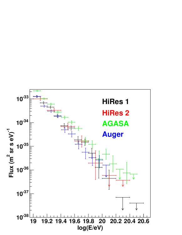
The most recent results disfavoring the GZK hypothesis come from the Akeno Giant Air Shower Array (AGASA) collaboration, whose published energy spectrum shows no indication of a high-energy suppression sasaki ; agasa . In contrast, the monocular-mode energy spectra measured by the High Resolution Fly’s Eye detectors (HiRes 1 and HiRes 2) support the existence of a GZK feature hiresI ; hiresII . The current world data set is still small. The AGASA claim that the GZK supression is not observed is based on only 11 events above $10^{20}$ eV. In the near future, the Pierre Auger Observatory, currently under construction in Malargue, Argentina, will dramatically increase the world data set. The Auger collaboration has published a first energy spectrum based on 1.5 years of data taken during construction auger1 .

A second problem is that although typically not shown in plots of the energy spectrum, the errors on the energy determination are also large: 30 % at $3\times 10^{19}$ eV and 25 % above $10^{20}$ eV in AGASA agasa , 30 % in HiRes hiresI ; hiresII and 50 % in Auger auger1 . Furthermore, a correct evaluation of the systematic errors is difficult. It should for example be noted that the systematic uncertainty for the AGASA energy scale includes a 10 % systematic uncertainty due to the hadronic model. This uncertainty is calculated by comparing different hadronic event generators and defining the systematic uncertainty by their difference. This may not be a reliable estimate of this uncertainty, which could potentially be much larger and is, in any case, unknown at this point. Since the AGASA and HiRes experiments use radically different techniques to determine the primary energy – AGASA is a ground array and HiRes an air fluorescence detector – the errors have fundamentally different sources.

The large statistical and systematic errors quoted by the experiments raise the question how much significance should be attached to the discrepancy between the HiRes and AGASA spectra. Several authors have addressed this question. In demarco1 ; demarco2 , the experimental results are compared individually to model predictions of the shape of the energy spectrum at GZK energies. Such an analysis requires assumptions on the nature of the cosmic ray sources, as the shape of the GZK suppression will of course depend on the source distribution.

Before one asks if any of the current measurements can be used as evidence for or against a specific model for the origin of cosmic rays, one needs to answer the question of whether or not the two experiments actually disagree at all, given their uncertainties. This requires a method to compare the two spectra that is both model-independent and considers the uncertainties quoted by the experiments by accounting for the probability of any systematic shift in energy scale applied to the data.

This paper presents a general spectrum comparison technique that for the first time addresses these points. The technique naturally incorporates the Poisson errors in the observed fluxes, and can probabilistically treat systematic errors in the absolute energy scale. The technique is developed in Section 2 and applied to the energy spectra of AGASA agasa , HiRes 1 and HiRes 2 in monocular mode hiresI ; hiresII and Auger auger2 in Section 3. Section 4 summarizes the results and describes how the method can be expanded for testing all experimental measurements against a theoretical prediction.

Figure 1: The AGASA agasa , Auger auger2 and HiRes monocular spectra hiresI ; hiresII .

II Proposed Comparison Between AGASA, HiRes and Auger

The comparison between the AGASA and HiRes spectra can be quantified as the relative probability that the various fluxes came from a signal parent distribution versus two separate distributions. This probability ratio is quantified as a Bayes Factor ($BF$). Two parent fluxes can arise for any number of reasons, for example systematic mismeasurement by either experiment, or – however unlikely – a different primary flux at AGASA or HiRes.

The calculation of the $BF$ is a variation of the method given in jeffreys comparing the consistency of two Poisson parameters. The statistic is the ratio of the probability that the spectra arise from separate parent distributions over the probability of the alternative hypothesis that they are derived from a single parent distribution. The $BF$ then indicates to what degree the separate parent hypothesis is favored. A widely accepted interpretation of the resulting value for the $BF$ is shown in Table 1.

To perform the calculation, we divide each energy distribution into $N$ bins. For the $i^{th}$ energy bin, the relative number of events is parametrized by the variable $f_{i}$. If the single-parent hypothesis is true, the relative exposures of the two experiments should determine the number of events expected from that single parent distribution. In the case of the two-parent hypothesis, a similar parameter, $f^{\prime}_{i}$, is invoked that can take any value for any bin and is not constrained by the relative exposures of the experiments. The probabilities of both hypotheses are calculated assuming Poisson uncertainties for the fluxes in the $i^{th}$ bin, while marginalizing the energy scale uncertainties.

Table 1: The interpretation of the separate parent flux hypothesis (SPFH) given the Bayes Factor ($BF$) jeffreys .

Bayes Factor ($BF$)	Interpretation
$BF>1$	SPFH supported
$10^{-\frac{1}{2}}<BF<1$	Minimal evidence against SPFH
$10^{-1}<BF<10^{-\frac{1}{2}}$	Substantial evidence against SPFH
$10^{-2}<BF<10^{-1}$	Strong evidence against SPFH
$BF<10^{-2}$	Decisive evidence against SPFH

We will derive the $BF$ using the comparison of the AGASA and HiRes spectra as an example; however, in the end, we will calculate a separate $BF$ for every combination of AGASA, HiRes 1, HiRes 2 and Auger spectra. The spectra for AGASA and HiRes at a given energy scale are defined as ${A_{i}}$ and ${H_{i}}$, where $i\in[1,N]$. We define the percent shift in the AGASA and HiRes energy scales to be $s_{A}$ and $s_{H}$, with the percent energy scale uncertainty to be $\sigma_{A}$ and $\sigma_{H}$, respectively. Following the derivation in jeffreys , the true number of events measured by AGASA and HiRes in the $i^{th}$ energy bin is parameterized by

$$a_{i}=f_{i}\eta_{i}$$ (1)

and

$$h_{i}=(1-f_{i})\eta_{i},$$ (2)

respectively, where $\eta_{i}$ is the total number of hypothesized events expected for both the AGASA and HiRes experiments. For the hypothesis where the two spectra come from a single parent distribution,

$$f_{i}=\frac{(AGASA~{}Exposure)_{i}}{(AGASA~{}Exposure)_{i}+(HiRes~{}Exposure)_{i}}.$$ (3)

In the case where the AGASA and HiRes experiments are measuring separate parent distributions, we parametrize the hypothesized events in a similar fashion. For the separate parent hypothesis,

$$a^{\prime}_{i}=f^{\prime}_{i}\eta_{i}$$ (4)

and

$$h^{\prime}_{i}=(1-f^{\prime}_{i})\eta_{i},$$ (5)

where $f^{\prime}_{i}$ is allowed to take any value and hence will be marginalized.

Making use of Bayes’ Theorem, the Bayes Factor is

$$BF = \frac{P(separate~{}parent~{}hypothesis|A,H)}{P(single~{}parent~{}hypothesis|A,H)}$$ (6)

$$= \frac{\int\int P(A,H|f^{\prime},\eta)q(f^{\prime},\eta)df^{\prime}d\eta}{\int P(A,H|f,\eta)q(f,\eta)d\eta}$$

where, e.g., $A\equiv\{A_{i}\}$. If one had a model with which to constrain $A$ and $H$, it would be included in the prior, $q(.)$. Any unknowns in the model could then be marginalized with $\eta_{i}$ and $f^{\prime}_{i}$ provided that the priors on $\eta_{i}$ and $f^{\prime}_{i}$ do not cancel. The denominator of Eq. (6) assumes some values for $f_{i}$ calculated through Eq. (3). The numerator marginalizes $f^{\prime}_{i}$ assuming any and all sets of $f_{i}^{\prime}$. By marginalizing over $f_{i}^{\prime}$, we are effectively asserting that the relative exposure quoted by the two experiments (defined by $f_{i}$) does not hold. Therefore, some adjustment needs to be made to one or both of the exposures. Since we do not have any idea what that adjustment could be, we sum over every possible relative exposure (i.e. marginalize $f_{i}^{\prime}$). Note: if the difference in the spectra are due to some physical process, this would manifest itself in a change in the relative exposures.

To introduce the energy scale uncertainties, we modify

$$P(A,H|f,\eta)q(f,\eta)\rightarrow P(A,H|f,\eta,s_{A},s_{H})$$

$$\times q(f,\eta,s_{A},s_{H})$$ (7)

to account for the deviations of the true energy scale from the mean energy scale of AGASA and HiRes, respectively. $A$ and $H$ are made dependent on the energy scale, such that the values of $A_{i}$ and $H_{i}$ will depend on $s_{A}$ and $s_{H}$, respectively. If the numerator and denominator are properly evaluated in this form, they necessarily account for the probability of some observed fluxes, $A$ and $H$, given the energy scale. As the deviations of the true energies from the measured energies are unknown, probability theory allows $s_{A}$ and $s_{H}$ to be marginalized such that Eq. (6) becomes

$$BF=\frac{\int\int\int\int P(A,H|f^{\prime},\eta,s_{A},s_{H})q(f^{\prime},\eta,s_{A},s_{H})df^{\prime}d\eta ds_{A}ds_{H}}{\int\int\int P(A,H|f,\eta,s_{A},s_{H})q(f,\eta,s_{A},s_{H})d\eta ds_{A}ds_{H}}.$$

The fluctuations in the fluxes are treated as Poisson, while the distributions of $s_{A}$ and $s_{H}$ are parametrized by Gaussians. Explicitly, the $BF$ is

$$BF= \frac{\int\int\left\{\prod_{i=1}^{N}\left[\int\int P_{f^{\prime}_{i}\eta_{i}}(A_{i})P_{(1-f^{\prime}_{i})\eta_{i}}(H_{i})df_{i}^{\prime}d\eta_{i}\right]\right\}N(s_{A};0,\sigma_{A})N(s_{H};0,\sigma_{H})ds_{A}ds_{H}}{\int\int\left\{\prod_{i=1}^{N}\left[\int P_{f_{i}\eta_{i}}(A_{i})P_{(1-f_{i})\eta_{i}}(H_{i})d\eta_{i}\right]\right\}N(s_{A};0,\sigma_{A})N(s_{H};0,\sigma_{H})ds_{A}ds_{H}}$$ (9)

where $P_{\mu}(M)$ denotes a Poisson distribution with mean $\mu$ and $M$ measured events and $N(x;\mu,\sigma)$ denotes a Gaussian with a deviation, $x$, from the mean, $\mu$, and error $\sigma$. By integrating $\eta_{i}$ within the product, we are effectively summing over every imaginable set of Poisson-distributed spectra. Each set of $A$ and $H$, where $A_{i}$ and $H_{i}$ are dependent on the energy shift, is weighted by the probability of that shift. Since the size of the shift toward the true energy scale is unknown, these shifts are marginalized by integrating $s_{A}$ and $s_{H}$. The numerator has an integration over $f^{\prime}_{i}$, effectively marginalizing over the cases where $A$ and $H$ come from different parent distributions.

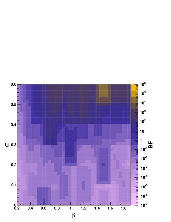
To get a sense of the behavior of the $BF$, we apply the method to a simple toy example. We generate two distributions, $S$ and $B$, each with 20 bins; distribution $S$ has 200 events, and distribution $B$ has $\beta\times 200$ events such that $f_{i}\equiv\frac{\beta}{1+\beta}$ where $f_{i}$ is identical for every bin. In effect, $\beta$ defines the relative exposures of the two “experiments” $S$ and $B$. The number of events in each bin of $S$ and $B$ fluctuates according to Poisson statistics.

On top of these “statistical” fluctuations, we introduce a second fluctuation of distribution $B$, while the mean of the $S$ distribution is kept flat. Each bin of the distribution $B$ is evenly fluctuated within $\pm\epsilon$, constraining the total events in $B$ to $200\times\beta$, thereby making the distributions more different as $\epsilon$ increases. Therefore, $\epsilon$ quantifies the disagreement between $S$ and $B$. Note that in contrast to the statistical fluctuations, these $\epsilon$ fluctuations are not included in the $BF$ and therefore deviations between $S$ and $B$ due to such fluctuations are ‘perceived’ by the $BF$ as differences in the spectra. We then plot the $BF$ as a function of $\beta$ and $\epsilon$ in Fig. 2.

The $BF$ distribution, given $\epsilon$ and $f$, has substantial tails that cause large fluctuations in Fig. 2 even when averaged over hundreds of thousands of trials. Despite these fluctutations, we are still able to pick out trends in the $BF$ as a function of $\beta$ and $\epsilon$. For instance, the $BF$ systematically increases with $\epsilon$ (i.e. as the difference between the distributions increases). As $\beta$ increases, the statistics for $B$ increase. Therefore, it is more likely that a given difference between two distributions is due to a real difference in the parents rather than low statistics.

Figure 2: $BF$ as a function of $\epsilon$ (the difference between the two parent distributions) and $\beta$ where the $BF$ is evaluated over two spectra with 200 and $200\times\beta$ events.

III Implementation

Due to practical limitations for the calculation of Eq. (9), some choices must be made in the binning and shifting of the data. The calculation occurs over 14 bins of size $\log{E/\mathrm{eV}}=0.1$ from $10^{19.6}$ eV to $10^{21.0}$ eV. The energy bins are determined from existing data. The $10^{19.6}$ eV cut-off is motivated by a previous comparison in demarco1 . The AGASA experiment has 866 events above $10^{19}$ eV and 72 above $10^{19.6}$ eV. HiRes 1 and HiRes 2 have 403 and 95 events above $10^{19}$ eV and 35 and 6 events above $10^{19.6}$ eV, respectively. Auger has 444 events above $10^{19}$ eV and 17 above $10^{19.6}$ eV.

After integrating over $f^{\prime}_{i}$ and $\eta_{i}$, Eq. (9) reduces to

$$BF=\frac{\int\int\left[\prod_{i=1}^{N}\frac{1}{A_{i}+H_{i}+1}\right]N(s_{A};0,\sigma_{A})N(s_{H};0,\sigma_{H})ds_{A}ds_{H}}{\int\int\left[\prod_{i=1}^{N}f_{i}^{A_{i}}(1-f_{i})^{H_{i}}\frac{(A_{i}+H_{i})!}{A_{i}!H_{i}!}\right]N(s_{A};0,\sigma_{A})N(s_{H};0,\sigma_{H})ds_{A}ds_{H}}$$ (10)

Since one cannot split a spectrum into an infinite number of bins, one must make finite shifts in the two energy spectra. The chosen shifts are made $\pm 5\sigma$ from the mean energy, and are incremented in $\log{E/\mathrm{eV}}=0.1$ steps, weighted by the Gaussians integrated over the energy bin. As various energy scales $s_{A}$ and $s_{H}$, are evaluated, the fluxes in the 14 bins change. The shifts $s_{A}$ and $s_{H}$ are evaluated down (up) to $\log{E/\mathrm{eV}}=-0.5$ ($\log{E/\mathrm{eV}}=0.5$). For instance, energy bins below $10^{19.6}$ eV shift in and out of the set of 14 bins depending on the values of $s_{A}$ and $s_{H}$. In the case of the HiRes 2 spectrum where the data are quoted in increments of $\log{E/\mathrm{eV}}=0.2$, the events are divided in proportion to the absolute size of the $\log{E/\mathrm{eV}}=0.1$ bin. Meanwhile, the relative exposures of AGASA and HiRes ($f$) remain unchanged.

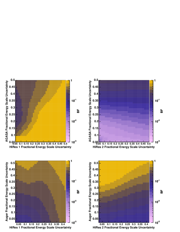
Fig. 3 shows the $BF$ as a function of the percent energy uncertainties for all combinations of AGASA, HiRes 1, HiRes 2 and Auger spectra. The distributions are non-trivial to understand as changing the energy scale does not amount to a simple shift in the number of events from one energy bin to another. Rather, in HiRes, the shape of the spectra change as the energy scale changes because the exposure remains fixed as a function of energy. Further, the probability that the spectra agree for a given energy scale is convoluted with the probability that that energy scale is the true energy scale for the detector. Meanwhile, the lower energy bins fall in and out of the calculation as the energy scales change in the course of the calculation.

If we compare AGASA and HiRes with $30\%$ energy scale uncertainties for both experiments, the $BF=0.71$ and $BF=0.04$ for HiRes 1 and HiRes 2, respectively. According to Table 1, the $BF$ for the HiRes 1 comparison corresponds to minimal evidence against the hypothesis that AGASA and HiRes are derived from separate distributions. The latter value for HiRes 2 corresponds to strong evidence against the separate source hypothesis. If we compare the Auger spectrum with 50 % energy scale uncertainties with the HiRes spectra with 30 % energy scale uncertainties, the $BF=0.54$ and $BF=0.85$ for HiRes 1 and HiRes 2, respectively, corresponding to minimal evidence against the separate source hypotheses (i.e. no support for the two-source hypothesis). Finally, if we compare the Auger spectrum with 50 % energy scale uncertainties with the AGASA spectrum with $30\%$ energy scale uncertainties we obtain a $BF=0.74$ again corresponding to minimal evidence against the separate source hypothesis.

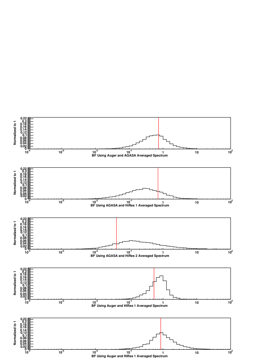
In order to verify that the $BF$ we obtain from the experimental data is indeed consistent with the single source hypothesis, we compare the actual $BF$ for the spectra from experiment $X$ and $Y$ to simulations of the $BF$ generated under the assumption that they are generated from a single parent.

To calculate a simulated $BF$ for the spectra from experiments $X$ and $Y$, we assume that the true spectrum is a spectrum that is an average, weighted by the exposure, of the spectra measured from experiments $X$ and $Y$. This average spectrum is then scaled to the corresponding exposures for $X$ and $Y$. We then randomly fluctuate both spectra according to Poisson statistics and calculate the $BF$. This procedure is repeated many times. The resulting distribution of the $BF$ for two spectra generated assuming a single parent is then compared to the experimental value of the $BF$ for the two measured spectra. Fig. 4 shows the results for a comparison of all three experiments with each other.

Figure 3: The Bayes Factor ($BF$) as a function of the percent energy scale uncertainties for the compared spectra.

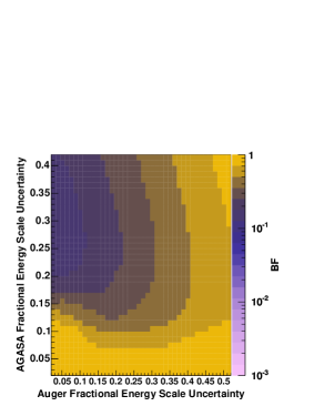
Comparing the $BF$’s measured for data (denoted by a red line) and those calculated in Fig. 4, we see that, in general, there is a substantial probability of obtaining a $BF$ that is larger than the $BF$’s calculated for the data. That is, a substantial number of samples that are derived from a single source look more like they were derived from two sources than the real AGASA, HiRes and Auger comparisons. The value of the $BF$ tells us that the hypothesis that the AGASA and HiRes energy spectra are consistent with a single distribution is favored over the hypothesis that they are derived from separate distributions.

Figure 4: The distribution of the $BF$ calculated for an averaged spectrum from two experiments. The red lines denote the $BF$’s measured for data.

IV Discussion

This result is similar to those obtained for the AGASA and HiRes spectra in demarco1 ; demarco2 by a rather different method. Our method directly compares two experimental results rather than comparing each to a theoretical prediction. It also treats systematic errors correctly by weighting possible systematic shifts in the energy distribution by the probability of that shift.

This result does not say anything about what the specific (in)consistencies would be of either experiment given a theory. However, our results indicate that there is room for a theory that agrees with each pair of spectra. As the statistical power of the world data improves, the methods discussed here will provide a convenient framework to compare experimental results with one another and with theoretical models.

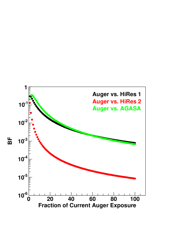
The Auger experiment is currently the only operating ultrahigh energy cosmic ray detector. The Auger data set will increase dramatically over the next years. Figure 5 shows the projected value of the $BF$ between Auger and the other experiments as a function of the fraction of the current Auger exposure. The $BF$ is calculated assuming the current spectra, the existing 30 % energy uncertainties in AGASA and HiRes and the projected 15 % energy uncertainties in the Auger spectrum. In the limit where the exposure for Auger becomes large, the $BF$ decreases (increasing support for the one-source hypothesis). That is, the statistical and energy scale uncertainties in HiRes and AGASA are so large that, barring a significant change in the Auger spectrum, one will never be able to tell whether or not the Auger and AGASA (HiRes) spectra are derived from different parent distributions provided that we limit our analysis to events above $10^{19.6}$ eV.

Figure 5: The projected $BF$ between the current Auger spectrum and the AGASA and HiRes spectra as a function of the fraction of the current Auger exposure. The calculations assume 30 % energy uncertainties in AGASA and HiRes and the projected 15 % energy uncertainties in the Auger spectrum.

Note, however, that if one fits a model to one of the experimental spectra, our result does not imply consistency of the model with the other experiment.

This project is supported by the National Science Foundation under contract NSF-PHY-0500492.

References

- (1) K. Greisen, Phys. Rev. Lett. 16, 748 (1966).
- (2) G.T. Zatsepin and V.A. K’uzmin, Pis’ma Zh. Eksp. Teor. Fiz. 4, 114 (1966) [JETP Lett. 4, 78 (1966)].
- (3) N. Sasaki et al., Proc. of ICRC 2001, 337 (2001).
- (4) M. Takeda et al., Astropart. Phys. 19, 447 (2003).
- (5) R.U. Abbasi et al., Phys. Rev. Lett., 92, 151101 (2004).
- (6) R.U. Abbasi et al., Astropart. Phys 23, 157 (2005).
- (7) Auger Collaboration, Proceedings ICRC, Puna, India 6 387 (2005), astro-ph/0507150.
- (8) Auger Collaboration, Proceedings ICRC, Puna, India 10 115 (2005), astro-ph/0604114.
- (9) D. De Marco, P. Blasi, and A.V. Olinto, Astropart.Phys. 20, 53 (2003).
- (10) D. De Marco, P. Blasi, and A.V. Olinto, J. Cosmol. Astropart. Phys. 01 (2006) 002.
- (11) H. Jeffreys Theory of Probability, Oxford University Press (1939).