Clustering of $K$-selected Galaxies at $2<z<3.5$: Evidence for a Color-Density Relation

Abstract

We study the clustering properties of $K$-selected galaxies at $2<z<3.5$ using deep multiwavelength imaging in three fields from the MUSYC survey. These are the first measurements to probe the spatial correlation function of $K$-selected galaxies in this redshift range on large scales, allowing for robust conclusions about the dark matter halos that host these galaxies. $K$-selected galaxies with $K<21$ have a correlation length $r_{0}\sim 6h^{-1}\textrm{Mpc}$, larger than typical values found for optically-selected galaxies. The correlation length does not depend on $K$-band magnitude in our sample, but it does increase strongly with color; the $J-K>2.3$ distant red galaxies (DRGs) have $r_{0}\sim 11h^{-1}\textrm{Mpc}$. Furthermore, contrary to findings for optically-selected galaxies $K$-selected galaxies that are faint in the $R$-band cluster more strongly than brighter galaxies. These results suggest that a color-density relation was in place at $z>2$; it will be interesting to see whether this relation is driven by galaxies with old stellar populations or by dusty star forming galaxies. Irrespective of the cause, our results indicate that $K$-bright blue galaxies and $K$-bright red galaxies are fundamentally different, as they have different clustering properties. Using a simple model of one galaxy per halo, we infer halo masses $\sim 5\times 10^{12}M_{\odot}$ for $K<21$ galaxies and $\sim 2\times 10^{13}M_{\odot}$ for DRGs. A comparison of the observed space density of DRGs to the density of their host halos suggests large halo occupation numbers; however, this result is at odds with the lack of a strong small-scale excess in the angular correlation function. Using the predicted evolution of halo mass to investigate relationships between galaxy populations at different redshifts, we find that the $z=0$ descendants of the galaxies considered here reside primarily in groups and clusters.

1. Introduction

Optical surveys of the high-redshift universe have been very successful in finding relatively unobscured star-forming galaxies, primarily via the $U$-dropout technique. These $z\sim 3$ Lyman break galaxies (LBGs) typically have stellar masses $\sim 10^{10}M_{\odot}$, star formation rates of $10-100M_{\odot}\textrm{yr}^{-1}$, and are thought to dominate the star formation density at that epoch (Steidel et al., 2003; Shapley et al., 2001; Reddy et al., 2005). However, it is becoming increasingly clear that substantial numbers of galaxies exist at these redshifts that have little rest-frame UV luminosity and are thus underrepresented in optical surveys. Such galaxies may be detected in the near-infrared (NIR), which samples the rest-frame optical.

One criterion used to select galaxies in the NIR is $J-K>2.3$ (Franx et al., 2003; van Dokkum et al., 2003). These distant red galaxies (DRGs) typically have high star formation rates, $\gtrsim 100M_{\odot}\textrm{yr}^{-1}$, and dust obscuration $A_{V}>1$, but must also have significant populations of evolved stars in order to explain their colors and spectra (Förster Schreiber et al., 2004; Papovich et al., 2006; Kriek et al., 2006a). Some DRGs show little or no evidence of active star formation (Labbé et al., 2005; Kriek et al., 2006a, b; Reddy et al., 2006). DRGs must in general be very massive to account for their significant $K$-brightness; stellar population synthesis models imply masses $M_{*}\sim~{}10^{11}M_{\odot}$. Indeed, $~{}95\%$ of galaxies with $M_{*}>10^{11}M_{\odot}$ at $2<z<3$ have $K<21.3$ (van Dokkum et al., 2006). Conversely, the median galaxy in this mass range has $R\sim 25.9$, fainter than the limits typically reached by optical surveys.

The relationship between $K$-selected samples and optically-selected samples, not to mention present-day galaxies, remains unclear. While typical optically-selected galaxies have different properties than $K$-selected galaxies, the $K$-bright subsample of optically-selected galaxies have stellar masses, star formation rates, and metallicities that are in approximate agreement with $K$-selected galaxies (Shapley et al., 2004; Reddy et al., 2005). Nevertheless, it is not clear whether the differences between these galaxies are transient (e.g. dust geometry, starbursts, mergers) or fundamental (e.g. age of the underlying old stellar populations, mass, environment). An understanding of the nature of the differences between populations is essential to place them in evolutionary scenarios.

One way to investigate differences between galaxy populations is to measure their clustering properties. As clustering measurements provide information that is independent of photometric properties, they can be used to distinguish between transient and fundamental differences between galaxy populations. In the halo model of galaxy formation, the large-scale distribution of galaxies is determined by the distribution of dark matter halos. The correlation function of galaxies can therefore be associated with the correlation function of the halos in which they reside. Halo clustering, in turn, is a strong function of halo mass (Mo & White, 1996), providing a means to study the relationship between galaxy properties and the mass of the dark matter halos.

Several studies have measured the dependence of clustering strength of high-redshift galaxies on color. Daddi et al. (2003) use the ultradeep imaging of the $4.5\textrm{arcmin}^{2}$ FIRES HDF-S field (Labbé et al., 2003) to study the clustering characteristics of $K$-selected galaxies at $2<z<4$. Their most striking finding is that the correlation length increases strongly with $J-K$ color, with the reddest galaxies in their sample having correlation lengths $r_{0}=10-15h^{-1}\textrm{Mpc}$, comparable to the most luminous red galaxies in the local universe. The mass of dark matter halos with similar correlation lengths is $>10^{13}M_{\odot}$, yet the galaxy number density is $\sim 100$ times larger than that expected for such massive dark matter halos, implying that many galaxies must share the same halo. More recently, Grazian et al. (2006) measured a $r_{0}=13.4^{+3.0}_{-3.2}h^{-1}\textrm{Mpc}$ for $z>2$ DRGs using the larger $135\textrm{arcmin}^{2}$ GOODS-CDFS field, also indicating that red galaxies are located in very massive halos.

The interpretation of these clustering measurements is complicated by the fact that, in order to derive information about the dark matter halos, the correlation function must be measured on large scales. The correlation function has a contribution from galaxies that share halos (hereafter the “1-halo” term) and galaxies in separate halos (the “2-halo” term). The shapes of these two contributions are shown with impressive detail in the correlation functions of large samples of $z\sim 4$ LBGs presented by Lee et al. (2006) and Ouchi et al. (2005). In order to derive meaningful constraints on large-scale clustering properties, and thus on the host dark matter halos, it is important that both of these terms are taken into consideration. If the correlation function is parameterized as a simple power-law then it should be measured on scales where the 2-halo term dominates the clustering signal. In practice, a firm lower limit to the radial range in which the angular correlation function should be fitted is the halo virial radius. At $z=3$, the virial radius $r_{200}$ of a $10^{13}M_{\odot}$ halo corresponds to $22\arcsec$ (e.g. Mo & White, 2002). The majority of the clustering signal from Daddi et al. (2003) and Grazian et al. (2006) is on scales $\theta\lesssim 30\arcsec$, which may lead to gross overestimates of the large-scale correlation length and the mass of the host dark matter halos. In particular, Zheng (2004) shows that the measurements of Daddi et al. (2003) are consistent with models in which the large-scale correlation length is as low as $r_{0}\sim 5h^{-1}$ and the typical halo mass is $\sim 10^{12}M_{\odot}$. This suggests that DRGs and LBGs may occupy similar halos, but that DRGs have higher occupation numbers.

The goal of this work is to study the clustering characteristics of a $K$-selected population of galaxies at $2<z<3.5$. The increased field-of-view of our imaging allows for an improved determination of the clustering strength of $K$-selected galaxies at angular separations sufficiently large to investigate the large-scale distribution of galaxies, and thus to provide more meaningful estimates of the masses of the halos in which they reside. Secondarily, we wish to analyze the clustering results using models of halo clustering, and to use these models to shed light on evolutionary scenarios for $z>2$ galaxies. These types of analyses have previously been performed for optically-selected samples (e.g. Moustakas & Somerville, 2002; Ouchi et al., 2004; Adelberger et al., 2005a). Throughout, we use the cosmological parameters $\Omega_{m}=0.3$, $\Omega_{\Lambda}=0.7$, $H_{0}=70h_{70}\textrm{ km}\textrm{ s}^{-1}\textrm{ Mpc}^{-1}$, and $\sigma_{8}=0.9$. Results are given using $h_{70}=1$, except for correlation lengths which are scaled to units of $h=0.7$ in order to facilitate comparison to previous studies. Optical magnitudes are given in AB and NIR magnitudes are given on the Vega system.

2. Data

The Multiwavelength Survey by Yale-Chile (MUSYC) consists of optical and NIR imaging of four independent $30\arcmin\times 30\arcmin$ fields plus spectroscopic follow-up (Gawiser et al., 2006, R. Quadri et al. 2006, in preparation). Deeper $JHK$ imaging was obtained over $10\arcmin\times 10\arcmin$ sub-fields with the ISPI camera at the CTIO Blanco 4m telescope. The present analysis is restricted to three of these deep fields (the adjacent HDFS1 and HDFS2, and SDSS 1030). The deep $JHK$ data will be described in detail elsewhere (R. Quadri et al. 2006, in preparation). The total $5\sigma$ point source limiting depths are $J\sim 23.0$, $H\sim 21.8$, and $K\sim 21.3$. The optical $UBVRIz$ data are described in Gawiser et al. (2006).

Figure 1.— The inferred redshift distribution of galaxies selected with $2<z_{\rm{phot}}<3.5$. The upper two curves are for the full sample, and the lower two curves are for galaxies that meet the $J-K>2.3$ criterion for DRGs. Dashed curves indicate the distribution of $z_{\rm{phot}}$ values, smoothed with a $\Delta(z)=0.4$ boxcar average. Solid curves indicate the distributions derived by summing the redshift probability distributions for each galaxy. The normalization is arbitrary.

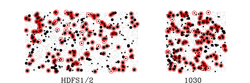
Figure 2.— The position of $K<21$ galaxies at $2<z_{\rm{phot}}<3.5$ in the deep MUSYC fields. The field sizes are $\sim 20\arcmin\times 10\arcmin$ and $\sim 10\arcmin\times 10\arcmin$ for HDFS1/2 and 1030, respectively. The large black circles represent galaxies with stellar mass $M_{*}>10^{11}M_{\odot}$ and the small black circles represent less massive galaxies. Galaxies that meet the $J-K>2.3$ criterion for distant red galaxies are marked with an open red circle.

In this study we use spectroscopic redshifts where possible, but must rely primarily on photometric redshifts. Photometric redshifts were determined using the methods of Rudnick et al. (2001, 2003). Briefly, non-negative linear combinations of galaxy templates are fit to the observed spectral energy distributions. The templates include the four empirical templates of Coleman, Wu, & Weedman (1980), as well as the two empirical starburst templates of Kinney et al. (1996), all of which have been extended into the UV and NIR using models. As the empirical templates are derived from low-redshift samples, we find that they do not adequately describe all $z\gtrsim 2$ galaxies. For this reason we added $10\textrm{Myr}$ and $1\textrm{Gyr}$ old single stellar population templates generated with the Bruzual & Charlot (2003) models. The redshift probability distribution for each galaxy is calculated using Monte Carlo simulations in which the observed fluxes are varied within the photometric uncertainties.

A comparison of the photometric redshifts to spectroscopic redshifts drawn from the literature and from our own observations yields a mean $\Delta z/{(1+z)}=0.12$ for $z>1.5$, corresponding to $\Delta z\sim 0.4$ at $z\simeq 2.5$. The dashed curves in Fig. 1 show the redshift distribution for all MUSYC galaxies with $2<z<3.5$, and for DRGs in the same redshift range. The solid curves show the distributions that are inferred by summing the redshift probability distributions. All distributions have been smoothed with a $\Delta z=0.4$ boxcar to limit spikes that, given our uncertainties, may not be real.

We restrict the sample to galaxies with $2<z_{\rm{phot}}<3.5$ and $K<21$, except where noted. Fig. 2 shows the positions of the DRGs in the three MUSYC fields. Also shown are galaxies with stellar mass $M_{*}>10^{11}M_{\odot}$, where $M_{*}$ is determined with stellar population synthesis models (§3.4.4).

3. The two-point correlation function

3.1. Method

The two-point correlation function can be measured by counting the number of unique galaxy pairs as a function of separation, and comparing the resultant distribution to that of a catalog of random points with the same number density and subject to the same observing geometry. Several estimators for the angular two-point correlation function are available, but the estimator introduced by Landy & Szalay (1993) is emerging as the de facto standard for high-redshift studies. It has been shown to minimize the variance and biases associated with other estimators (Landy & Szalay, 1993; Hamilton, 1993; Kerscher et al., 2000). The observed amplitude of the two point correlation function is thus

$$w_{obs}(\theta)=\frac{DD(\theta)-2DR(\theta)+RR(\theta)}{RR(\theta)},$$ (1)

where $DD(\theta)$ is the number of data-data pairs with angular separation in the interval $(\theta-\Delta\theta/2,\theta+\Delta\theta/2$). $DR(\theta)$ is the number of data-random pairs, and $RR(\theta)$ is the number of random-random pairs, in the same angular interval. We use $\Delta\theta=20\arcsec$. In order to better sample the observing geometry, and to decrease the uncertainty in $DR(\theta)$ and $RR(\theta)$, we use $\sim 100$ times more random points than data points. This requires normalizing the $DR$ and $RR$ terms such that $\sum_{\theta}DR(\theta)=\sum_{\theta}RR(\theta)=\sum_{\theta}DD(\theta)$.

The angular correlation function can be approximated as a power law

$$w(\theta)=A_{w}\theta^{-\beta}.$$ (2)

However, as the (suitably normalized) number of random pairs is equal to the number of data pairs, and since the two-point correlation function is the excess probability of finding a data pair versus a random pair, it is clear that $w_{obs}(\theta)$ cannot be positive for all $\theta$. In particular,

$$\int\int w_{obs}(\theta_{12})d\Omega_{1}d\Omega_{2}\approx 0.$$ (3)

This integral constraint requires that $w_{obs}(\theta)$ fall below the intrinsic $w(\theta)$ (Groth & Peebles, 1977). The size of this bias increases with the clustering strength and decreases with field size; in practice, it is a significant effect and a correction must be made. The integral constraint correction is approximately constant and equal to the fractional variance of galaxy counts in a field,

$$IC\approx\sigma^{2}=\frac{1}{<N_{gal}>}+\sigma_{w}^{2},$$ (4)

where the first term on the right is the Poisson variance and the second accounts for the additional variance caused by clustering

$$\sigma_{w}^{2}=\frac{1}{\Omega^{2}}\int\int w(\theta_{12})d\Omega_{1}d\Omega_{2}$$ (5)

(Peebles, 1980, §45). Although the clustering term dominates the integral constraint, the Poisson term is non-negligible for the small sample sizes considered here. Following Infante (1994) and Roche et al. (1999) the clustering term $\sigma_{w}^{2}$ can be estimated numerically using

$$\sigma_{w}^{2}=\frac{\sum_{i}A_{w}\theta_{i}^{-\beta}RR(\theta_{i})}{\sum_{i}RR(\theta_{i})}.$$ (6)

The quantity $\sigma_{w}^{2}/A_{w}$ is estimated directly from the random catalog for an assumed value $\beta$. The amplitude $A_{w}$ of the angular correlation function is related to the observations through the fitting function

$$w_{obs}(\theta)=A_{w}\theta^{-\beta}-IC.$$ (7)

We estimate $A_{w}$ iteratively using eqs. 6, 4, and 7. The final result is robust against differences in the initial estimate of $A_{w}$ and convergence only takes a few iterations.

In the weak clustering regime the uncertainty in the Landy & Szalay estimator can be estimated by assuming that $DD(\theta)$ has Poisson variance (Landy & Szalay, 1993); in this case

$$\delta w_{obs}(\theta)\approx\frac{1+w(\theta)}{\sqrt{DD(\theta)}}.$$ (8)

If the angular correlation function is a power law, the spatial correlation function will also be a power law

$$\xi(r)=\left(\frac{r}{r_{0}}\right)^{-\gamma},$$ (9)

where $r_{0}$ is the spatial correlation length and ${\gamma=\beta+1}$. The angular correlation function can be used to obtain the spatial correlation function by inverting the Limber projection

$$A_{w}=\frac{H_{\gamma}r_{0}^{\gamma}\int F(z)r_{c}^{1-\gamma}(z)N^{2}(z)E(z)dz}{(c/H_{o})(\int N(z)dz)^{2}},$$ (10)

where $r_{c}(z)$ is the comoving radial distance, N(z) is the redshift distribution,

$$H_{\gamma}=\Gamma(1/2)\frac{\Gamma[(\gamma-1)/2]}{\Gamma(\gamma/2)},$$ (11)

and

$$E(z)=\sqrt{\Omega_{m}(1+z)^{3}+\Omega_{\Lambda}},$$ (12)

(e.g. Magliocchetti & Maddox, 1999).

The function $F(z)$ describes the evolution of clustering with redshift, $\xi(r,z)=\xi(r,0)F(z)$. The evolution has often been modelled as $F(z)=(1+z)^{-(3-\gamma+\epsilon)}$, where the parameter $\epsilon$ is typically specified using $\epsilon=\gamma-3$ for constant clustering in comoving units, $\epsilon=0$ for ‘stable clustering’, or $\epsilon=\gamma-1$ for ‘linear growth’ (e.g. Moscardini et al., 1998; Overzier et al., 2003). We assume constant clustering in comoving units over $2<z<3.5$; this sets $F(z)=1$. Different values of $\epsilon$, where the correlation length is then determined at the median redshift of the observed sample, yield similar results.

3.2. Measurement Strategies

In what follows we restrict the analysis to galaxies with photometric redshift $2<z_{\rm{phot}}<3.5$. Reducing the redshift range produces comparable correlation lengths, but with larger uncertainties. Additionally, as we largely rely on photometric redshifts, we cannot be confident in our ability to divide the sample too finely in redshift space.

It is common practice in the literature to assume $\gamma=1.8$ if the data are not sufficient to make independent measurements of both the slope and the amplitude of the correlation function. Recent studies have found that $\gamma\sim 1.6$ may be more appropriate for LBGs (Adelberger et al., 2005a; Lee et al., 2006). Direct comparisons of the correlation length from different studies can be problematic unless the same $\beta$ was used; for this reason, the results summarized below use $\gamma=1.8$ but Tables 1 and 2 also gives the $r_{0}$ values corresponding to $\gamma=1.6$.

In placing the random objects on the image, we mask out regions where galaxies could not be detected, e.g. in the vicinity of bright stars. This procedure makes a negligible change in the resultant correlation functions.

We measure $w_{obs}(\theta)$ (eq. 1) in linearly-spaced $20\arcsec$ bins for the purpose of computing the $\chi^{2}$ fits. Spacing the bins at equal logarithmic intervals gives similar results for most samples considered here. We present the results of power law fits over the range $0\arcsec<\theta<200\arcsec$ in Table 1, and $40\arcsec<\theta<200\arcsec$ in Table 2. Most of the discussion and analysis in this paper is based on the latter fits. The $200\arcsec$ upper limit minimizes the effects of low level biases (such as errors in the flat-fielding and the integral constraint) and edge effects. The $40\arcsec$ lower limit is set so that the fit is not strongly affected by 1-halo term of the correlation function (§4). At $z=2$, the minimum redshift of our sample, $40\arcsec$ subtends $0.7h^{-1}\textrm{Mpc}$ in comoving units, which corresponds to the virial radius $r_{200}$ of an $\sim 3\times 10^{13}M_{\odot}$ halo. This is roughly the mass of halos that host the most clustered galaxies in our sample (§4), and is larger than the scales ($<10\arcsec$; $<0.25h^{-1}\textrm{Mpc}$) at which $z\sim 4$ LBGs show significant contributions from the 1-halo term (Ouchi et al., 2005; Lee et al., 2006). For reference, Adelberger et al. (2005a) uses a lower limit of $60\arcsec$, but our reduced signal-to-noise does not allow for such a conservative limit. In contrast, Grazian et al. (2006) fit $w(\theta)$ over $1\arcsec<\theta<100\arcsec$. Neither Grazian et al. (2006) nor Daddi et al. (2003) significantly constrain $w(\theta)$ beyond $40\arcsec$ (see their Figs. 9 and 8, respectively).

We note that, for most samples considered here, the $0\arcsec<\theta<200\arcsec$ fits result in correlation lengths that are larger than the $40\arcsec<\theta<200\arcsec$ correlation lengths by $\sim 1-1.5\sigma$. For some subsamples the $0\arcsec<\theta<200\arcsec$ correlation lengths are actually smaller, although the difference is always $\leq 1\sigma$.

While performing the fit at large scales reduces the effect of the 1-halo term on the correlation length, there is a second-order effect of the halo occupation distribution that we do not take into account. A fully consistent treatment would require counting only one galaxy per halo, to avoid counting the same halo more than once. As we have no robust method to detect galaxies that share halos, halos that host multiple galaxies will be counted multiple times when measuring $w(\theta)$. Since only the most massive halos are likely to host multiple galaxies, these halos effectively receive more weight. Our data are not sufficient to address these second-order effects, and we note that simply rejecting all galaxies that have close neighbors would introduce other biases in our measurements.

3.3. Sources of uncertainty

3.3.1 Redshift distribution

The shape of the redshift distribution $N(z)$ in eq. 10 will affect the deprojection of the angular two point correlation function, contributing to the uncertainty in $r_{0}$. One strategy for dealing with the redshift uncertainties is to smooth the $z_{\rm{phot}}$ distribution by the typical uncertainty, $\Delta z\sim 0.4$ (§2). However, it is likely that the redshift uncertainties differ for different galaxies in our sample. This may affect the observed relationships between galaxy properties and clustering strength; for instance, if faint galaxies have a larger photometric redshift uncertainty than bright galaxies, their intrinsic redshift distribution may be wider. In this case, smoothing with the same $\Delta z$ will not sufficiently broaden the redshift distribution of faint galaxies, resulting in an underestimate of the correlation length of faint galaxies for some observed value of $A_{w}$. This will introduce an artificial trend of increasing clustering with increasing brightness. We note that many other studies of galaxy clustering–which use the same redshift selection function for all galaxy samples–may be subject to this effect.

A more appropriate redshift distribution for use in eq. 10 may be had by summing the redshift probability distribution $P(z)$ (see §2) for each galaxy in the sample. To the extent that our Monte Carlo simulations provide an accurate estimate of $P(z)$, this strategy circumvents the problem of choosing a smoothing width. Additionally, we compute $\sum P(z)$ separately for each sub-sample under consideration, thereby reducing the problem of differential redshift uncertainties.

The smoothed $z_{\rm{phot}}$ distributions are narrower than the (more realistic) $\sum P(z)$ distributions that are used throughout this paper. We note that using these narrower distributions would reduce our estimates of $r_{0}$ by $\sim 15-25\%$, where the more clustered populations display the smaller differences. In the case of DRGs, about half of the $\sim 15\%$ difference between these two estimates of $r_{0}$ comes from the $z<1.8$ tail of the $\sum P(z)$ distribution, and the other half comes from the broader overall distribution at $z>1.8$ (Fig. 1).

If redshift interlopers are assumed to be randomly distributed they will dilute observed angular correlation by a factor $(1-f_{c})^{2}$, where $f_{c}$ is the contamination fraction. One method to account for interlopers is to estimate $f_{c}$ using the redshift probability distributions, and to calculate a contaminant-corrected $r_{0}$ by integrating over the range $1.8<z<3.5$ in eq. 10. As the assumption of a random distribution is probably unrealistic, we choose instead to account for interlopers by integrating over the entire redshift range. The correlation lengths are similar regardless of the method used.

3.3.2 Field to Field Variance

The Landy & Szalay estimator has been shown to have approximately Poisson variance in the limit of zero clustering (Landy & Szalay, 1993), but a clustered population is expected to show covariance between the radial bins (Bernstein, 1994). The deep NIR MUSYC survey consists of only two independent fields (HDFS1/2 and 1030), so field to field variations will present an additional source of error. Moreover, uncertainty in the integral constraint is not correctly accounted for by Poisson statistics. Here we estimate the confidence intervals of our results with simulated data sets. Our approach is similar in spirit to that described by Daddi et al. (2003).

We construct a clustered population using outputs from the public GalICS simulations (Hatton et al., 2003). GalICS uses cosmological N-body simulations to trace the growth and merging of dark matter halos, and a semi-analytic approach to follow the formation and evolution of galaxies within the halos. The simulations use $8.272\times 10^{9}M_{\odot}$ particles in a $100h^{-1}\textrm{Mpc}$ simulation box, $\Omega_{m}=0.333$, $\Omega_{\Lambda}=0.667$, $h=0.667$, and $\sigma_{8}=0.88$. The GalICS outputs are available in convenient ‘observing cone’ catalogs (Blaizot et al., 2005) that mimic what an observer would see in a simulated universe. The limited size of the simulation box requires replication of galaxies within the observing cones. Although the observing cone geometry has been tuned to reduce replication effects, precise measurements of galaxy clustering and the cosmic variance are hampered by replication effects.

We construct $27$ mock data sets from the eight $1\textrm{deg}^{2}$ GalICS observing cones. Each of these mock data sets has the same geometry and field sizes as the deep NIR MUSYC survey, and we measure the clustering of the simulated galaxies using the same methods. The results are used to estimate the $68\%$ confidence range of the amplitude $A_{w}$ of the angular correlation function. More detailed characterizations of the uncertainties would require larger simulations. The confidence range is a function of both intrinsic clustering, which is adjusted by selecting galaxies with different halo mass, and surface density, which is adjusted by randomly removing galaxies. For most of the samples here, $\sigma_{A_{w}}/A_{w}\approx 55\%-70\%$–significantly larger than the Poisson values alone. This does not imply that our results are only significant at the $\lesssim 2\sigma$ level, as populations with small $A_{w}$ will have small $\sigma_{A_{w}}$, and so populations with little or no clustering rarely show strong clustering (see also Fig. 1 of Daddi et al., 2003). We will return to this issue in §3.4.2 for the specific case of DRG vs. LBG clustering.

The errors due to field to field variations are reduced when comparing populations of galaxies drawn from the same fields, so we quote Poisson uncertainties except where noted. The estimated total uncertainty in the correlation length due to both Poisson errors and field to field variance is given in the last column of Table 2. We note that most studies of galaxy clustering at high redshift do not fully account for the effects of field to field variance.

3.4. Results

3.4.1 Angular and spatial clustering of galaxies with $2<z_{\rm{phot}}<3.5$

Fig. 3 shows the angular correlation function for $K$-selected galaxies with $2<z_{\rm{phot}}<3.5$ and $K<21$. The correlation function is roughly consistent with a power law down to $\sim 1\arcsec$, the approximate resolution limit of our survey. There is a slight indication of an excess on smaller scales: the amplitude of the best-fitting power law $A_{w}=1.9\pm 0.3$ when the fit is restricted to $\theta<200\arcsec$ and $A_{w}=1.3\pm 0.4$ over $40\arcsec<\theta<200\arcsec$. Lee et al. (2006) and Ouchi et al. (2005) also note that the best-fitting power law changes for smaller angular intervals for their sample of $z\sim 4$ LBGs. Although our sample is not large enough to trace the detailed shape of $w(\theta)$, it is possible that this is evidence of the small-scale excess that is predicted by halo occupation distribution models (e.g. Wechsler et al., 2001; Zheng, 2004). However, as emphasized by Adelberger et al. (2005a), the observation that approximate power law behavior extends to such small scales may itself be interpreted as evidence that galaxies share halos. The solid line in Fig. 3 shows the expected shape of the angular correlation function of dark matter halos $w_{h}(\theta)$, derived using N-body simulations (§3.3.2). Halo exclusion effects force $w_{h}(\theta)$ to flatten on smaller scales. In the case of one galaxy per halo, $w(\theta)$ should follow $w_{h}(\theta)$. If galaxies have a higher probability than halos of having close neighbors, then it is likely that some fraction of these galaxy neighbors reside in the same halo. We return to this point in §4.

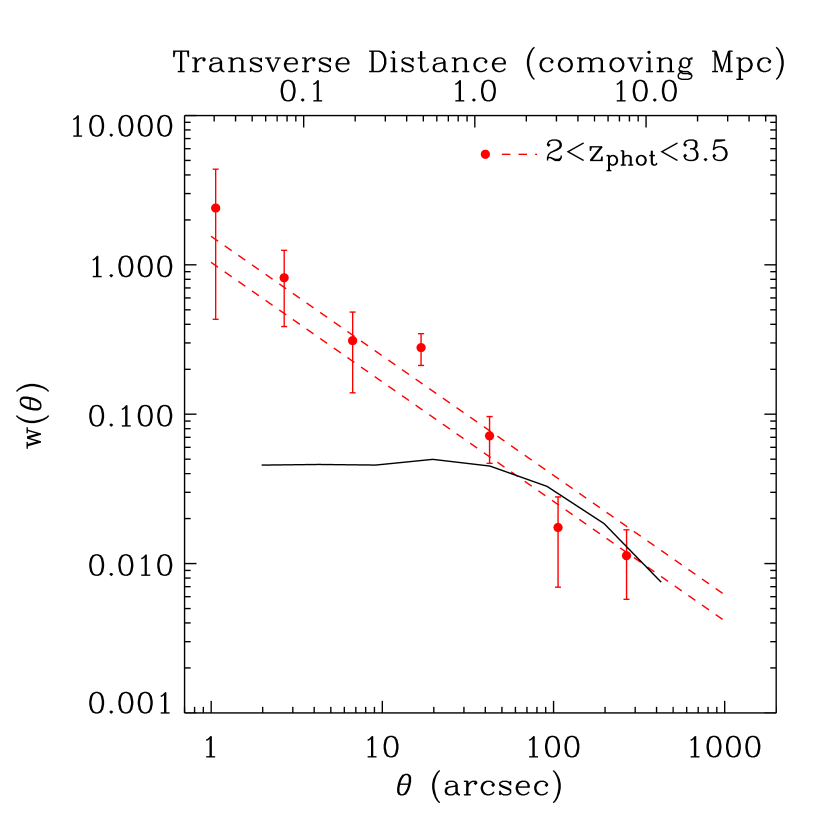
Figure 3.— The angular correlation function, with the integral constraint correction applied to the data points, for galaxies with $2<z_{\rm{phot}}<3.5$ and $K<21$. The upper x-axis shows the transverse comoving distance at the median redshift $z=2.6$. The dashed lines show the best fit power laws over $\theta<200\arcsec$ (upper) and $40\arcsec<\theta<200\arcsec$ (lower). The lower fit is preferred in order to reduce the effects of halo substructure in $w(\theta)$. The solid curve illustrates the shape of the angular correlation function that is expected for dark matter halos; the larger values of the galaxy correlation function at small separations suggest that some halos host multiple galaxies.

We invert the angular correlation function $w(\theta)$ to derive the spatial correlation length $r_{0}$ using eq. 10. Restricting the fit to the angular range $40\arcsec<\theta<200\arcsec$, we find $r_{0}=6.0^{+0.9}_{-1.1}h^{-1}\textrm{Mpc}$ (comoving). For comparison, the correlation lengths of $R<25.5$ optically-selected $z\sim 2-3$ BX galaxies and LBGs is $\sim 4h^{-1}\textrm{Mpc}$ (Adelberger et al., 2005a; Lee et al., 2006). The latter use a power law slope of the correlation function $\gamma\simeq 1.6$, whereas we use $\gamma=1.8$. Assuming $\gamma=1.6$ increases the correlation length of MUSYC galaxies to $r_{0}=6.6^{+1.0}_{-1.1}h^{-1}\textrm{Mpc}$. The larger correlation lengths for $K$-selected sample might have been expected, as $K$-bright galaxies have been shown to cluster more strongly than optically-selected $K$-faint galaxies at $z\sim 2$ (Daddi et al., 2004; Adelberger et al., 2005b). This dependence on selection filter may reflect underlying trends with $K$-magnitude, color, mass, or other parameters; these issues are discussed in the following subsections (see particularly §3.4.3).

3.4.2 Clustering as a function of color

Fig. 4 compares the angular correlation function of DRGs with $J-K>2.3$ to that of non-DRGs with $J-K<2.3$, in the redshift range $2<z_{\rm{phot}}<3.5$ and with $K<21$. The DRGs cluster more strongly than the bluer galaxies at large scales. The angular correlation function of DRGs is roughly consistent with a power law down to $\sim 4\arcsec$, which corresponds to the virial radius of a $\sim 10^{11}M_{\odot}$ halo. For the blue galaxies, $w(\theta)$ remains consistent with a power law to $\sim 1\arcsec$. The two $w(\theta)$ data points at $\theta<4\arcsec$ correspond to $1$ and $8$ observed blue galaxy pairs respectively, whereas the DRGs have $0$ and $2$ pairs at these small separations. Extrapolating the power law fit to these scales, we would expect only $1$ and $4$ galaxy pairs for the DRG sample. While galaxy pairs at separations approaching $40\arcsec$ may share the same halo, it is not clear whether or not they will eventually merge. However galaxies with these significantly smaller separations ($4\arcsec$ corresponds to a projected distance of $36$ proper kpc at $z=2.6$) should be interacting strongly and could be mergers in progress. The lack of close DRG pairs may therefore indicate that DRGs are undergoing few mergers. Whether this is because DRGs are the products of recent mergers, or because merger-induced star formation makes the red galaxies bluer, or whether there is some other explanation, is unknown. Evaluating the significance of the lack of close DRG pairs is severely complicated by galaxy deblending issues in our $\sim 0.9\arcsec$ FWHM images, and we will not discuss this issue further.

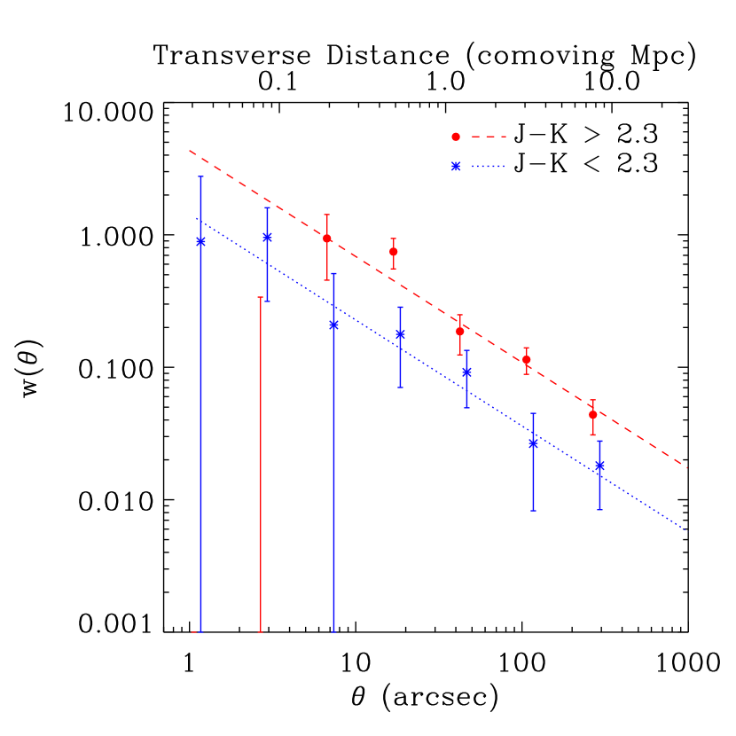
Figure 4.— The angular correlation function for $2<z_{\rm{phot}}<3.5$ galaxies that meet the $J-K>2.3$ threshold for distant red galaxies (DRGs), and for non-DRGs. A small horizontal offset has been applied to the blue points for display purposes only. The power law fits to $w(\theta)$ are performed at $40\arcsec<\theta<200\arcsec$ to reduce the effects of halo substructure in $w(\theta)$.

We find $r_{0}=11.1^{+1.3}_{-1.4}h^{-1}\textrm{Mpc}$ for DRGs. Note that, if the full field to field variance is taken into account, we estimate $r_{0}=11.1^{+2.8}_{-4.2}h^{-1}\textrm{Mpc}$. If the fit is performed over $\theta<200\arcsec$, then $r_{0}=12.0^{+0.9}_{-1.0}h^{-1}\textrm{Mpc}$ (Poisson errors only). These values are consistent with the $r_{0}=13.4^{+3.0}_{-3.2}h^{-1}\textrm{Mpc}$ given by Grazian et al. (2006) and $r_{0}=14.5^{+3.1}_{-3.7}h^{-1}\textrm{Mpc}$ given by Daddi et al. (2003), although the latter authors do not apply a photometric redshift cut.

Fig. 5 shows the comoving correlation length as a function of minimum $J-K$ color threshold. We confirm the previous result of Daddi et al. (2003) that the redder galaxies cluster more strongly, even though their result was derived using a single $\sim 4.5\textrm{ arcmin}^{2}$ field, and they measure $w(\theta)$ at $\theta\lesssim 70\arcsec$ (see their Fig. 8). It should also be noted that their sample reaches $2-3$ magnitudes deeper than ours, and it is not obvious that the same trends should hold over such a wide luminosity range. There is a slight trend of increasing median redshift with increasing $J-K$ color, but the difference is $\approx 0.1$ over the range of colors studied here, so it is unlikely that the relationship between color and $r_{0}$ is solely due to redshift evolution. We note that alternate galaxy colors, such as $R-K$, are also strongly correlated with clustering (Fig. 6). LBGs and BX galaxies have a correlation length $r_{0}\approx 4h^{-1}\textrm{Mpc}$ (Adelberger et al., 2005a; Lee et al., 2006), lower than the value for the bluest threshold shown in Fig. 5, although the brightest $R<24$ LBGs reach $r_{0}=7.8\pm 0.5h^{-1}\textrm{Mpc}$ (Lee et al., 2006). The median $J-K$ color of $z\sim 3$ LBGs is $\sim 1.6$ (Shapley et al., 2001), and very few LBGs/BX galaxies reach the reddest thresholds (Reddy et al., 2005; van Dokkum et al., 2006).

We have established the significance of the increased clustering with color in several ways. Splitting our sample at the median color, $J-K\sim 2.17$, we find $r_{0}=11.0^{+1.1}_{-1.2}h^{-1}\textrm{Mpc}$ and $r_{0}=6.1^{+1.8}_{-2.5}h^{-1}\textrm{Mpc}$ for the redder and bluer sample, respectively. We then randomly split the sample of $K$-selected galaxies in two repeatedly, measuring the correlation length each time. The correlation length reaches as high as $r_{0}=11h^{-1}\textrm{Mpc}$ only $\sim 4\%$ of the time, indicating that we have established the stronger clustering for redder samples at the $\sim 96\%$ level. We have also used the simulations described in §3.3.2 to see how often a population with the same correlation length as LBGs, but number density and redshift distribution similar to what we infer for DRGs, can have a measured correlation length as high as that observed for DRGs as a result of field to field variations; we found that this only happens $\sim 5\%$ of the time. Futhermore, we have verified that the increase in clustering with color is not driven by any one of our three ISPI fields by repeating the clustering measurements three times, each time removing one of the fields; although the exact values of the correlation length vary, the relationship between clustering and color is always present. Finally, we recall that the ‘total’ uncertainties, which include the estimated contribution from field to field variations and are presented in Table 2, overestimate the uncertainties when comparing correlation lengths of galaxies that are drawn from the same fields.

The increasing clustering with color indicates that a color-density relationship was in place at $z\gtrsim 2$. In the local universe, this relationship is understood as an effect of higher metallicity and higher stellar ages in the densest regions; both effects may play a role at high redshift (Förster Schreiber et al., 2004; van Dokkum et al., 2004; Shapley et al., 2004). The high dust obscuration associated with vigorous starbursts also contributes to the red colors of many $K$-selected galaxies (e.g. Förster Schreiber et al., 2004; Labbé et al., 2005; Webb et al., 2006). It is entirely possible that the dusty and the “red and dead” galaxies (Kriek et al., 2006b) have different clustering properties, but the strong relationship between $J-K$ and $r_{0}$ suggests that neither of these populations is weakly clustered. Disentangling the relationship between clustering and star formation for red galaxies would likely require large fields with Spitzer Space Telescope observations (Labbé et al., 2005).

Figure 5.— The comoving correlation length for $2<z_{\rm{phot}}<3.5$ galaxies redder than the $J-K$ color threshold.

Figure 6.— The comoving correlation length for $2<z_{\rm{phot}}<3.5$ galaxies redder than the $R_{AB}-K_{Vega}$ color threshold.

3.4.3 Clustering as a function of apparent magnitude

Fig. 7 shows the relationship between correlation length and minimum $K$-magnitude. There is a small trend with the fainter galaxies clustering more strongly, but the significance of this effect is low; removing either the HDFS1 or HDFS2 fields from this analysis eliminates this relationship, while removing 1030 actually increases it. We conclude that the data do not suggest a strong relationship between $K$ and $r_{0}$. This contrasts with results from $z\sim 2.3$ BX objects, which show clustering that increases strongly with $K$ (Adelberger et al., 2005b); we comment further on this below. The bottom panel of Fig. 7 shows that the fraction of red galaxies—where here we characterize a galaxy as red if it has $J-K$ larger than the median—does not vary significantly with $K$. Combined with the result that $r_{0}$ correlates with $J-K$, it appears that color, and not $K$-magnitude, is the primary determinant of clustering strength.

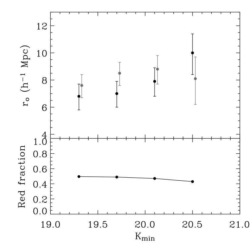
Figure 7.— The upper plot shows the comoving correlation length for galaxies fainter than a $K$-magnitude threshold. The grey points show the results from the HDFS1 and 1030 fields only; these points have been offset in the horizontal direction for clarity. The lower plot shows that the fraction of red galaxies (defined as galaxies redder than the median, $J-K\geq 2.17$) does not change strongly over this magnitude range.

Next we split the sample into two populations using an apparent optical magnitude cut $R=25$, which is approximately equal to the median total $R$-magnitude, and is $0.5$ magnitudes shallower than the limit used for $z\sim 3$ LBGs (Steidel et al., 2003). Fig. 8 shows that the optically brighter $K$-selected subsample clusters less strongly than the fainter subsample. This result is at odds with several studies of optically selected galaxies, including BX objects at $z\sim 2.3$ (Adelberger et al., 2005a), LBGs at $z\sim 3$ (Giavalisco & Dickinson, 2001; Foucaud et al., 2003; Adelberger et al., 2005a; Lee et al., 2006), and LBGs at $z\sim 4$ and $z\sim 5$ (Lee et al., 2006; Ouchi et al., 2004), all of which display stronger clustering with increased rest-frame UV luminosity. It is interesting that our brighter subsample has a correlation length that agrees well with R-selected samples in the same magnitude range. Thus our results suggest that the $K$-selected galaxies that are below the limits of current $R$-selected surveys are the most strongly clustered.

We note that the median $K$-magnitudes of our two subsamples are similar–with the optically-faint sample $0.1$ magnitudes brighter than the optically-bright sample–and the overall distributions of $K$-magnitude are also similar. So the anti-correlation between $r_{0}$ and $R$-brightness may simply be a manifestation of the correlation between $r_{0}$ and the $R-K$ color (Fig. 6). Similarly, the observations of Shapley et al. (2005) suggest a relationship between $R-K$ and $K$ for BX objects, and Adelberger et al. (2005b) speculate that the observed relationship between $r_{0}$ and $K$ for their sample may reflect an underlying correlation between $r_{0}$ and $R-K$. Thus the results for both $K$-selected galaxies and optically-selected galaxies suggest that color may be the most important driver of clustering strength. If this is the case, the difference in colors between these two populations may explain the difference in clustering properties, as $K$-selected galaxies tend to be redder.

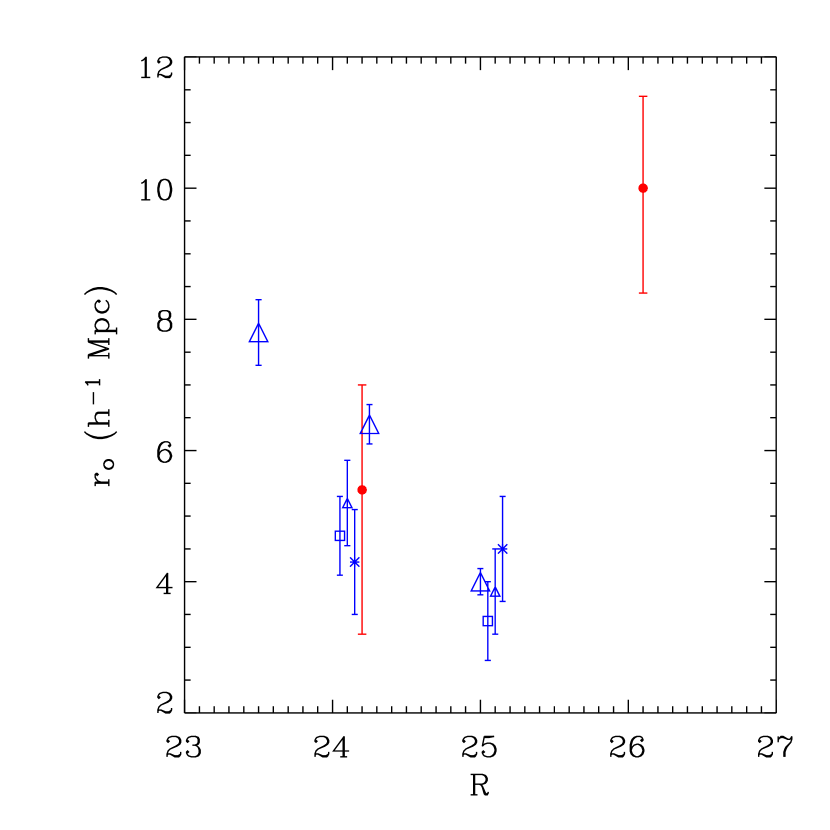
Figure 8.— The comoving correlation length for $R$-selected (blue symbols) and $K$-selected galaxies (red circles), shown at representative $R$-magnitude values. The large triangles are for $z\sim 3$ LBGs from Lee et al. (2006). The small triangles are LBGs at $z\sim 3$, the squares are BX objects at $z\sim 2.3$, and the asterisks are BM objects at $z\sim 1.7$, all taken from Adelberger et al. (2005a). The LBGs and BX objects show increasing clustering with increasing $R$-brightness, whereas the BM objects show no apparent trend, and the $K$-selected MUSYC galaxies appear to show the opposite trend.

3.4.4 Clustering as a function of stellar mass

To investigate the relationship between stellar mass and clustering, we estimate the mass of MUSYC galaxies by fitting Bruzual & Charlot (2003) models to the observed photometry at fixed $z_{\rm{phot}}$. We assume a $\tau=300\textrm{Myr}$ declining star formation history, solar metallicity, and a $0.1-100M_{\odot}$ Salpeter (1955) initial mass function.

Fig. 9 shows that the angular correlation function of galaxies with $M_{*}>10^{11}M_{\odot}$ and for galaxies with $M_{*}<10^{11}M_{\odot}$ are very similar. The top panel of Fig. 10 shows the correlation length vs. minimum stellar mass threshold. There is no clear trend. The bottom panel of Fig. 10 shows that the fraction of red galaxies is an increasing function of mass threshold. It was shown above that $r_{0}$ increases strongly with $J-K$ color; from this it might be expected that clustering would increase strongly with mass, because the most massive galaxies tend to be red. Moreover, the median masses of the $R$-faint and $R$-bright samples in Fig. 8 are $6.2\times 10^{10}M_{\odot}$ and $1.6\times 10^{11}M_{\odot}$, again suggesting a possible relationship between mass and $r_{0}$. So it is interesting that we do not observe a clear relationship between clustering and stellar mass, although it must be noted that the data shown in Fig. 10 have large error bars.

As discussed by van Dokkum et al. (2006), the majority ($\sim 65\%$ in the current sample) of $M_{*}>10^{11}M_{\odot}$ galaxies at $z>2$ are DRGs. With such significant overlap between the massive and red galaxies, it is to be expected that they have similar correlation lengths. However, we find $r_{0}=5.9^{+1.8}_{-2.4}h^{-1}\textrm{Mpc}$ for $M_{*}>10^{11}M_{\odot}$ galaxies, and $r_{0}=11.1^{+1.3}_{-1.4}h^{-1}\textrm{Mpc}$ for DRGs. This indicates that either the massive non-DRGs have a very low correlation length, or that the less massive DRGs have a very high correlation length. Our sample is not large enough to investigate each of these sub-populations individually, but we do note that the correlation length for galaxies that are both massive and meet the $J-K>2.3$ criterion for DRGs is $r_{0}=7.9^{+1.9}_{-2.4}h^{-1}\textrm{Mpc}$, intermediate between the massive and DRG samples. This may be evidence that the low-mass DRGs are highly clustered and that the high-mass blue galaxies are less clustered. Relative to the median high mass DRG, the median low mass DRG is fainter in the NIR ($K=20.8$ vs. $20.3$), brighter in the optical ($R=25.8$ vs. $27.1$), but has a similar NIR color ($J-K=2.6$ vs. $2.7$). We have verified that it is not $K$-faint DRGs which contribute so strongly to the clustering but rather it is the low-mass DRGs by measuring $r_{0}=10.5^{+1.6}_{-1.8}h^{-1}\textrm{Mpc}$ for $K<20.7$ DRGs. This result is analogous to conclusions from the local universe, where low-mass red galaxies and high-mass red galaxies inhabit the densest environments (Hogg et al., 2003; Kauffmann et al., 2004), and to the fact that, among massive galaxies, there is a strong relationship between correlation length and optical color (Li et al., 2006). Additionally, Kauffmann et al. (2004) show that the stellar mass of galaxies is not a strong function of halo mass in the most massive halos.

It should be noted that, while we are approximately complete for galaxies with $M_{*}>10^{11}M_{\odot}$ (van Dokkum et al., 2006), we will be very incomplete for less massive galaxies. Using stellar mass estimates from the ultradeep FIRES MS 1054-03 field (Förster Schreiber et al., 2006), we estimate $\sim 65\%$ completeness for galaxies with $M_{*}>10^{10.4}M_{\odot}$. Scatter in our mass measurements may also obscure any relationship between $r_{0}$ and mass. Significantly deeper data are needed to study the dependence of $r_{0}$ on mass for a complete sample.

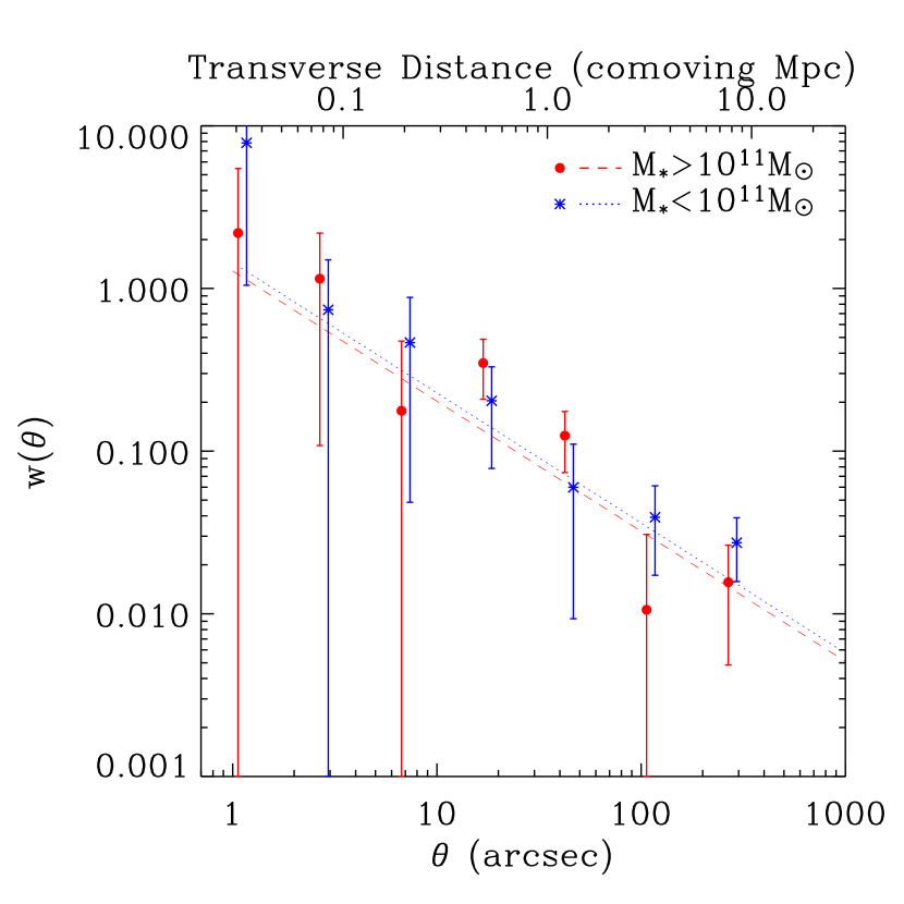
Figure 9.— Same as Fig. 4, for mass-selected samples.

Figure 10.— The comoving correlation length as a function of stellar mass threshold. The lower plot shows the fraction of red galaxies (defined as galaxies redder than the median, $J-K\geq 2.17$) as a function of mass.

4. Relationship between galaxies and dark matter halos

In the halo model of galaxy formation, the galaxy correlation length is related to the mass of dark matter halos (Mo & White, 1996). In this section we constrain the halo masses and occupation numbers of the various subsamples of MUSYC galaxies using the measured correlation lengths and number densities.

4.1. The number density and bias of dark matter halos

To investigate the relationship between the MUSYC $K$-selected galaxies and dark matter halos, we use the halo mass function of Sheth & Tormen (1999) that is derived from fits to large N-body simulations

$$\frac{dn_{h}}{dM}=A\left(1+\frac{1}{\nu^{\prime 2q}}\right)\sqrt{\frac{2}{\pi}}\frac{\bar{\rho}}{M}\frac{d\nu^{\prime}}{dM}\exp\left(\frac{-\nu^{\prime 2}}{2}\right),$$ (13)

where $\nu^{\prime}=\sqrt{a}\delta_{c}/\sigma(M,z)$, and the constants $\delta_{c}\approx 1.69$, $a=0.707$, $A\approx 0.322$, $q=0.3$, and $\bar{\rho}$ is the current mean mass density of the universe. We calculate the relative mass fluctuations in spheres that contain an average mass $M$ as

$$\sigma(M,z)=D(z)\sigma(M,0),$$ (14)

where $D(z)$ is the growth factor for linear fluctuations given by Carroll et al. (1992), and $\sigma(M,0)$ is calculated using a scale-free $n=1$ initial power spectrum and the transfer function of Bardeen et al. (1986).

The linear halo bias is calculated using the function of Sheth, Mo, & Tormen (2001)

$$b_{h}=1+\frac{1}{\delta_{c}}\left[\nu^{\prime 2}+b\nu^{\prime 2(1-c)}-\frac{v^{\prime 2c}/\sqrt{a}}{\nu^{\prime 2c}+b(1-c)(1-c/2)}\right],$$ (15)

where $b=0.5$ and $c=0.6$. Further details can be found in e.g. Mo & White (2002).

Several definitions of the bias–which relates the clustering of objects to that of the overall dark matter distribution– in terms of observable quantities appear in the literature. We choose

$$b=\frac{\sigma_{8,gal}}{\sigma_{8}(z)},$$ (16)

where $\sigma_{8}(z)$ is the variance in $8h^{-1}\textrm{Mpc}$ spheres and is calculated analogously to eq. 14. If the galaxy correlation function $\xi(r)$ is a power-law of the form eq. 9 then it can be integrated to give the relative variance

$$\sigma_{8,gal}^{2}=\frac{72}{(3-\gamma)(4-\gamma)(6-\gamma)2^{\gamma}}\left(\frac{r_{0}}{8h^{-1}\rm{Mpc}}\right)^{\gamma}$$ (17)

(Peebles, 1980, §36, §59).

We model the simple case of one galaxy per halo above a minimum halo mass threshold, i.e. a halo occupation number of 1. More detailed models, such as setting the halo occupation number equal to a power law above some mass threshold (e.g. Wechsler et al., 2001) are beyond the scope of this paper. As we measure the bias of the galaxy samples at scales larger than $\sim 1\textrm{Mpc}$, we can associate the observed bias with the linear bias of the host halos calculated with eq. 15, thereby providing an estimate of the halo mass.

Fig. 11 shows the average halo bias (weighted by the number density) and number density as a function of halo mass threshold at the median redshift, $z\simeq 2.6$. The $1\sigma$ bias range for DRGs, as well as the minimum mass and the number density of halos with the same bias values, is illustrated by the shaded region. From this figure we can read off the mass threshold of halos that have the same bias as DRGs, $M_{h}\approx 1.5-3\times 10^{13}M_{\odot}$. The larger sample of $K<21$ galaxies has $M_{h}\approx 1.5-5\times 10^{12}M_{\odot}$. For comparison, the LBGs and BX galaxies occupy halos with mass threshold $M_{h}\approx 10^{11.5}M_{\odot}$ and $\approx 10^{12}M_{\odot}$, respectively (Adelberger et al., 2005a) .

4.2. The halo occupation number

In the local universe, halos with mass $\lesssim 10^{12}M_{\odot}$ tend to have only one bright galaxy, whereas $\gtrsim 10^{14}M_{\odot}$ halos may contain dozens (e.g. Kauffmann et al., 2004). There is also evidence of galaxies sharing halos at high redshift (Daddi et al., 2003; Zheng, 2004; Adelberger et al., 2005a; Ouchi et al., 2005; Lee et al., 2006). We define the mean halo occupation number $N_{occup}$ as the ratio of galaxy number density to the number density of host dark matter halos. Occupation numbers greater than unity suggest that multiple galaxies can reside in a single halo.

The simplest estimate for the number density of galaxies comes from dividing the observed number of galaxies by the volume probed by our survey at $2<z<3.5$. However there may be significant evolution of the actual number density over this redshift range, and there is probable contamination by interlopers. We attempt to correct for these effects by estimating the fraction of the observed galaxies that lie at $z\sim 2.6$ using the redshift distributions discussed in §2. We note that these two estimates agree to within the field-to-field variance within the survey, which is $\sim 20\%$. The estimated number density of galaxies at $z\sim 2.6$ with $K<21$ is $(5\pm 2.5)\times 10^{-4}h_{70}^{3}\textrm{Mpc}^{-3}$. For DRGs, we estimate $(2\pm 1)\times 10^{-4}h_{70}^{3}\textrm{Mpc}^{-3}$. GOODS-CDFS – the only other public field with size, depth, and multiwavelength coverage comparable to one of our fields – shows a lower density of massive and red galaxies than are present in the MUSYC survey, indicating that our field-to-field variance may not be representative (van Dokkum et al., 2006; Grazian et al., 2006). Incompleteness and possible systematics in photometric redshifts further complicate density estimates; we therefore assign approximate $50\%$ uncertainties. These number densities are consistent with estimates from the luminosity function (Marchesini et al., 2006).

Fig. 12 compares the number density and correlation lengths for various samples to the values that are expected in the case of a one-to-one relationship between galaxies and dark matter halos. As noted by e.g. Adelberger et al. (2005a), the observed properties of $z\sim 3$ LBGs are roughly consistent with such a relationship. The same is true for the entire MUSYC $K$-selected sample, as well as the sample of $M_{*}>10^{11}M_{\odot}$ galaxies. However the redder galaxies deviate strongly from the expected relation, suggesting high occupation numbers. In particular, the number density of halos with the same bias as DRGs is $\approx 2.4-13\times 10^{-6}h_{70}^{3}\textrm{Mpc}^{-3}$, suggesting $N_{occup}\approx 40^{+60}_{-30}$. However, if the estimated field to field variance is taken into account (Table 2), the DRGs may have a correlation length as low as $r_{0}\approx 7h^{-1}\textrm{Mpc}$, in which case $N_{occup}\sim 1$. The bright $K<20.5$ BX galaxies from Adelberger et al. (2005b) also suggest high occupation numbers, although the very strong clustering in one of their observed fields may drive their result.

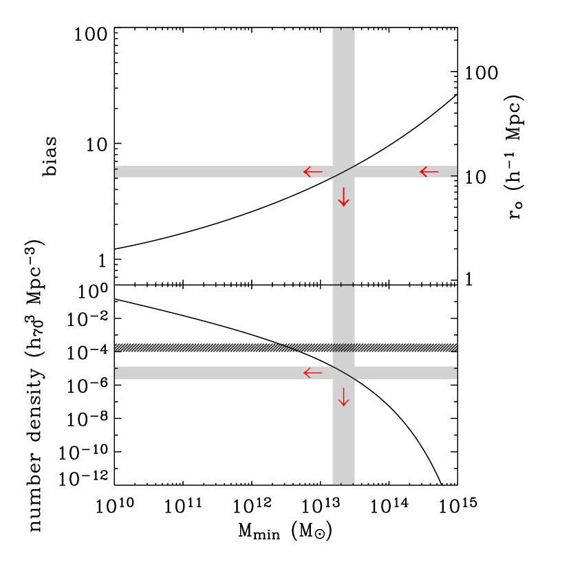
Figure 11.— Upper: The number-weighted average linear bias as a function of minimum halo mass threshold at $z=2.6$. The right axis shows the relationship between galaxy correlation length and the inferred large-scale galaxy bias. The shaded regions show the $1\sigma$ range of allowed $r_{0}$, and the corresponding range in bias and halo mass. Lower: The comoving halo number density as a function of halo mass threshold. The shaded regions show the $1\sigma$ range of mass and number density for the halos that host DRGs. The hatched region shows the observed number density of DRGs, illustrating that they are $40^{+60}_{-30}$ times more numerous than the halos that host them.

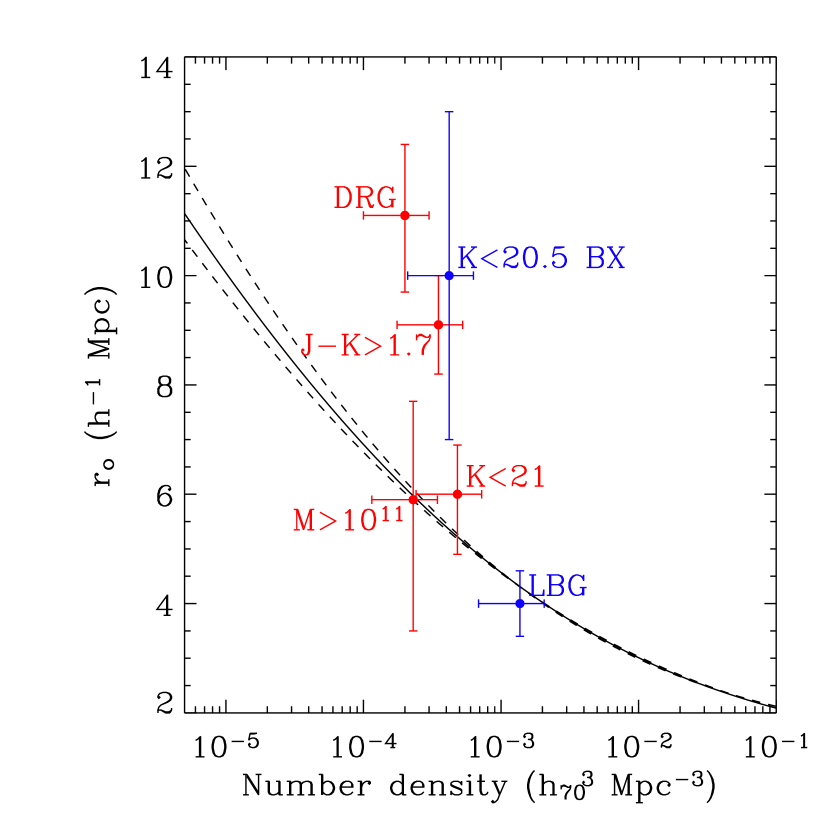
Figure 12.— The correlation length and the number density of different populations of $z>2$ galaxies. The LBG data are taken from Adelberger et al. (2005a). The $r_{0}$ for the $K$-bright BX galaxies is taken from Adelberger et al. (2005b). We estimate the number density of bright BX galaxies by using density of all BX galaxies given by Adelberger et al. (2005a) and applying a correction using the information given in Adelberger et al. (2005b). The solid line shows the approximate correlation length $r_{0}$ as a function of number density that would be expected in the case of one galaxy per halo at $z=2.6$; the upper and lower dashed lines show the same information at $z=3$ and $z=2$, respectively. Although the inferred halo mass for a galaxy population with a given $r_{0}$ will depend on the redshift of the galaxy population, the relationship between $r_{0}$ and number density for dark matter halos is not a sensitive function of redshift.

4.3. Constraining the occupation number with the number of close pairs

In the previous subsection we estimated the occupation number $N_{occup}$ using the standard method of comparing the observed number density of galaxies to the number density of their host halos. If many galaxies share the same halo, then the angular positions of galaxies should show strong ‘clumps,’ i.e. the correlation function should indicate large power on small scales. Here we obtain an independent estimate of $N_{occup}$ by comparing the shape of the angular correlation function $w(\theta)$ to the angular correlation function of dark matter halos $w_{h}(\theta)$.

Although the angular and spatial correlation functions of dark matter halos are well-approximated by power laws on scales larger than $\sim r_{vir}$, the probability of finding distinct halos with separation $<r_{vir}$ necessarily falls to $0$; this sets $\xi_{h}(r<r_{vir})\sim-1$. However, for a sufficiently large redshift selection window, $w_{h}(\theta)$ will tend to remain flat on small angular scales because of projection effects (see Fig. 3). The extent to which the galaxy correlation function $w(\theta)$ differs from the $w_{h}(\theta)$ on small scales can be used to constrain the occupation number (Wechsler et al., 2001; Bullock, Wechsler, & Somerville, 2002; Adelberger et al., 2005a).

The expected number of galaxies in the angular interval $(0,\theta_{max})$ around a randomly-chosen galaxy is

$$N=n_{g}\pi\theta_{max}^{2}(1+w_{<\theta_{max}}),$$ (18)

where $n_{g}$ is the mean surface density of galaxies, and $w_{<\theta_{max}}$ is the value of the angular correlation function evaluated over the same angular interval (i.e. using eq. 1 and a bin of width $\theta_{max}$). This relation follows directly from the definition of the angular correlation function. If all galaxies are associated with halos, and if $\theta_{max}$ is larger than the virial radius, the average number of galaxies within the same angular interval is the number of additional galaxies within the host halo plus a contribution from neighboring halos,

$$N\approx f+N_{occup}n_{h}\pi\theta_{max}^{2}(1+w_{h,<\theta_{max}}),$$ (19)

where $f$ denotes the average number of additional galaxies in a halo that hosts at least one galaxy. Note that $N_{occup}=n_{g}/n_{h}$, so the right hand side of eq. 19 does not depend directly on $N_{occup}$. Combining eqs. 18 and 19 gives an estimate of $f$ that depends on both $w(\theta)$ and $w_{h}(\theta)$ over the interval $(0,\theta_{max})$, as well as on $n_{g}$. Under the assumption that all halos above the minimum mass threshold host detectable galaxies, it is apparent that $N_{occup}=(f+1)$. If some fraction $g$ of these halos do not host detectable galaxies, then $N_{occup}$ is reduced by a factor $(1-g)$. There is some indication that $g>0$ for LBGs (Adelberger et al., 2005a; Lee et al., 2006). Here we make the simplifying assumption that $g=0$, which is consistent with the $N_{occup}\gtrsim 1$ measurements from the previous subsection, and note that the $N_{occup}$ measurements of this section may be upper limits.

We measure $w_{h,<\theta_{max}}$ directly from the observing cone output of the GalICS simulations (see §3.3.2), using halos with a large-scale angular correlation and redshift distribution similar to those inferred for our sample. Because the GalICS observing cone outputs do not specify the coordinates of halos, we instead use the coordinates of the most central galaxy in each halo when measuring the correlation functions. As shown in Fig. 3, $w_{h}(\theta)$ flattens over the region $\theta\lesssim 40\arcsec$. Our results are relatively insensitive to the details of this procedure, and the uncertainties are dominated by the uncertainties in $w(\theta)$ and in the galaxy surface density $n_{g}$, which we estimate from the observed variance among the MUSYC fields. We use the observed field-to-field variations to estimate the uncertainty in $n_{g}$, and use $\theta_{max}=60\arcsec$ in eqs. 18 and 19.

We derive $N_{occup}\approx 1.7\pm 0.3$ for DRGs. Other galaxy subsamples have occupation numbers that are consistent with the DRG value to within $1\sigma$. In the previous subsection we showed that the observed correlation lengths and number densities suggest $N_{occup}\sim 1$ for the $K<21$ and $M_{*}\sim~{}10^{11}M_{\odot}$ galaxies, consistent with the values derived here. However, the value for DRGs is much less than the $N_{occup}=40^{+60}_{-30}$ that is inferred from the correlation length. This may indicate that our measured correlation length is an overestimate. Possible causes for this discrepancy are given in §6, however we note that these values are consistent if the estimated field-to-field variance in the correlation length is taken into account (§3.3.2 and Table 2). Previous studies have found correlation lengths even larger than ours (Daddi et al., 2003; Grazian et al., 2006), although their measurements may have been unduly influenced by small-scale structure in $w(\theta)$ (§3.4, and Zheng, 2004).

In the previous subsection we showed that the number density and correlation length of $K<20.5$ BX galaxies (Adelberger et al., 2005b) point toward very high occupation numbers. However these authors indicate that their results do not change significantly if they include galaxy pairs at small separations in their analysis. This suggests that there is no evidence of a strong small-scale excess in their correlation functions, and therefore that bright BX galaxies also show a disagreement between their observed properties and the properties of dark matter halos, although the difference is not as significant as for DRGs.

5. Relating galaxy populations at different redshifts

5.1. Evolution of galaxy bias

What are the $z=0$ descendants of the $K$-selected galaxies discussed in this paper? In the $\Lambda\textrm{CDM}$ picture of structure formation, the large-scale distribution of galaxies is determined primarily by the dark matter potential wells. Thus we can address the evolution of high-redshift galaxies by following the evolution of their host dark matter halos. Fortunately, the dynamics of collisionless dark matter particles are well-described by simple models or by cosmological N-body simulations. So while the complicated physics that dictates the evolution of the baryonic component of galaxies (e.g. star formation, feedback, mergers) cannot be addressed by these models or simulations alone, we can constrain the bias and halo mass of the $z=0$ descendants.

One way to investigate relationships between galaxy populations at different redshifts is to compare their observed bias. As the universe evolves with time, the dark matter becomes more clustered and the bias of a set of biased objects will decrease. The bias $b(z)$ of a set of test particles evolved according to

$$b(z)=1+(b(0)-1)/D(z)$$ (20)

(Fry, 1996) where $D(z)$ is the growth factor. It is important to note that this equation does not account for merging and the evolution of the baryonic components of galaxies. Merging will play a role if galaxies in the densest (i.e. most biased) regions of space are more likely to merge than galaxies in less dense regions, thereby reducing the average bias of unique descendants. So it is possible that the bias will evolve faster than indicated by eq. 20. We refer to this as the ‘galaxy-conserving’ model of bias evolution. Fig. 13 shows tracks of bias evolution, along with the bias of different samples of galaxies (which we compute in a consistent way, using eq. 16). This figure shows that the brightest LBGs at $z\sim 3$ ($R<24$; Lee et al., 2006) have a bias roughly consistent with the $z\sim 2.6$ $K<21$ galaxies studied here. At higher redshift, only the brightest $z\sim 4$ LBGs ($i^{\prime}<24.8$; Ouchi et al., 2004; Allen et al., 2005) show biasing consistent with the lower-redshift DRGs, but the fainter $z\sim 4$ LBGs are not consistent.

Fig. 13 shows that all of the high-redshift samples discussed in this paper, including LBGs, evolve into highly-biased populations at $z\sim 0$. This point has been made previously for the optically-selected populations (e.g. Baugh et al., 1998; Ouchi et al., 2004; Adelberger et al., 2005a). Among the known galaxies at $z\sim 2$, it appears that only those that are faintest in $K$ can be progenitors of typical $L_{*}$ field galaxies.

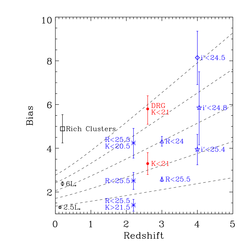
Figure 13.— The evolution of bias with redshift. The tracks show the evolution of bias calculated using the galaxy-conserving model, eq. 20. The filled red circles are based on this work, while the blue symbols are for optically-selected galaxies at various redshifts and black symbols are for local galaxies. The asterisks show the bias of BX galaxies from Adelberger et al. (2005a, b). The triangles show the bias of $z\sim 3$ LBGs from Lee et al. (2006). The diamond and stars are for the $z\sim 4$ LBGs of Allen et al. (2005) and Ouchi et al. (2004), respectively. Open circles are from Zehavi et al. (2005). The square represents the richest cluster sample analyzed by Bahcall et al. (2003). In all cases, we have calculated the bias using eqs. 16 and 17.

5.2. Evolution of halo mass

The preceding analysis only illustrates the bias of the descendants of high-redshift galaxies. If the galaxies within a given population follow different evolutionary paths, then the descendants will have diverse properties, and the average bias will have limited interpretive value. Knowledge of the range of environments or halo masses of the descendants is more meaningful. For a more detailed investigation of the $z=0$ descendants of $z>2$ galaxies, we track the growth of dark matter halos using cosmological N-body simulations. We choose the GIF simulation for its size and mass resolution, and for the publicly available halo catalogs and merger trees (Frenk et al., 2000). This simulation uses $\Omega_{m}=0.3$, $\Omega_{\Lambda}=0.7$, $h=0.7$, $\Gamma=0.21$, and $\sigma_{8}=0.9$. The linear size is $141.3h^{-1}$ comoving Mpc. A minimally-resolved halo consists of 10 particles with mass $1.4\times 10^{10}h^{-1}M_{\odot}$, but we note that the merging histories of halos less massive than $\sim 100$ particles may be inaccurate (Kauffmann et al., 1999).

In these simulations, the position of a central galaxy within a halo is given by the position of the most-bound dark matter particle. When halos merge, the central galaxy of the most massive progenitor becomes the new central galaxy while the central galaxy of less massive progenitors, as well as any progenitor satellites, are kept as satellites in the descendant halo. We assume that the galaxies in the present sample begin as central galaxies in $z\sim 2.6$ halos more massive than the threshold masses given in the previous subsection, and follow the positions of these galaxies to $z=0$. Occasionally satellite galaxies are ejected during mergers and may not be contained in any of the simulated halos at later times, however this effect occurs rarely for the massive halos considered here, and may be safely ignored. Additionally, we exclude halos near the edges of the simulation from analysis.

We note that our treatment of halo evolution is different than that of many other authors, and these differences may lead to contrasting conclusions. For instance, Grazian et al. (2006) employ the ”merging model” of Matarrese et al. (1997) and Moscardini et al. (1998) as one method to study the clustering evolution of DRGs. In the context of this model, $z=0$ galaxies are considered to be descendants of DRGs if they occupy halos that are more massive than the $z>2$ DRG host halos. More halos will meet this mass threshold at $z=0$ than at $z>2$, so many of these descendants enter the sample at intermediate redshifts, leading to a lower typical descendant halo mass. In this section we are concerned only with the direct descendants of $z\sim 2.6$ MUSYC galaxies.

There is an essential ambiguity in interpreting the range of halo masses occupied by the descendants of high-redshift galaxies. The simulations show that–because of halo mergers–many $z=0$ halos host multiple descendants. However it is unclear whether the galaxies themselves merge or whether they retain separate identities within a single halo. First we deal with the scenario in which the galaxies do not merge, as in the galaxy-conserving model discussed above. The red hatched region in Fig. 14 shows the $68\%$ range of host halo masses for descendants of high-redshift galaxies, as a function of halo mass at $z\sim 2.6$. The descendants of DRGs primarily occupy cluster-scale halos, with mass $\gtrsim 10^{14}M_{\odot}$. If our estimate of the correlation lengths for DRGs is correct, then DRGs with $K<21$ cannot be progenitors of the majority of local field early-type galaxies. It follows that DRGs exist in proto-cluster regions. The majority of LBGs also end up in group and cluster-scale halos. The black hatched region in Fig. 14 shows the mass range of halos occupied by descendants under the assumption that all galaxies within a single halo merge. In this case the most massive halos at $z=0$, which host multiple descendants of high-redshift galaxies, are only counted once. The difference between the two hatched regions illustrates the importance of merging; for instance, $\gtrsim 50\%$ of the halos that are inferred to host LBGs merge with a more massive halo between $z\sim 3$ and $z\sim 0$. This indicates either that LBGs tend to merge with more massive galaxies to form the brightest central galaxy in a halo, or that LBG descendants are satellites rather than the brightest central galaxy in these halos. It may be possible that some of the progenitors of the low-mass red galaxies that exist in dense regions (e.g. Hogg et al., 2003) are LBGs, although this would require star formation to cease shortly after the epoch of observation.

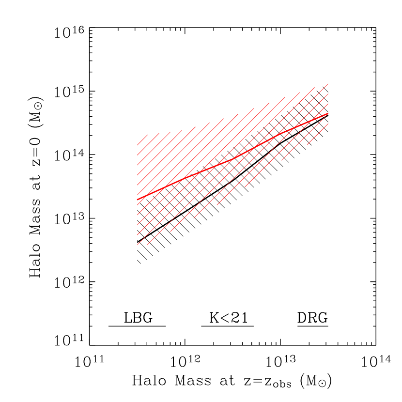
Figure 14.— The evolution of halo mass with redshift. The x-axis shows the halo mass at the redshift of observation, and the y-axis shows the mass of the descendant halos at z=0. The red hatched region indicates the predicted $68\%$ halo mass range for the descendants of $z\sim 2.6$ galaxies under the assumption of no galaxy mergers. The black hatched region indicates the mass range under the assumption that all galaxies that share halos merge. See the text for details. The thick solid curves show the median halo masses under each of these scenarios. The horizontal lines at the bottom of the figure mark the range of halo masses inferred for LBGs (Adelberger et al., 2005a), $K<21$ galaxies, and DRGs at the epoch of observation.

6. Summary and Discussion

We have used $300\textrm{arcmin}^{2}$ of $UBVRIzJHK$ imaging from the MUSYC survey to study the angular and spatial correlation functions of $K$-selected galaxies with $2<z_{\rm{phot}}<3.5$ and $K<21$. The correlation length for this sample is $r_{0}=6.0^{+0.9}_{-1.1}h^{-1}\textrm{Mpc}$, $\sim 50\%$ larger than optically-selected galaxies at similar redshifts (Adelberger et al., 2005a; Lee et al., 2006). The clustering of galaxies increases strongly with $J-K$ and $R-K$ color, and the $J-K>2.3$ population of distant red galaxies has $r_{0}=11.1^{+1.3}_{-1.4}h^{-1}\textrm{Mpc}$. Our results for DRGs are lower than previous results (Daddi et al., 2003; Grazian et al., 2006). This may be partially due to our smaller uncertainties. Additionally, previous studies were only able to constrain the correlation function on small scales, where the signal may be strongly affected by galaxies that share the same halo (Zheng, 2004; Ouchi et al., 2005; Lee et al., 2006). In contrast, we perform fits to the correlation function on scales larger than the typical halo virial radius where this effect is reduced.

Nevertheless we confirm the basic trend indicated by previous studies, in which red galaxies are much more strongly clustered than optically-selected galaxies. Moreover, this trend is not simply due to the fact that the red galaxies used in the previous studies were selected in the $K$-band: clustering increases strongly with color even within our $K$-selected sample, while there is no significant relationship between $K$-magnitude and color or between $K$-magnitude and correlation length. These results suggest that a color-density relationship was in place at $z>2$, as is also indicated by the properties of optically-selected galaxies in different environments (Steidel et al., 2005). Whether this relationship is driven by galaxies that are red because of dust obscuration, or because of low specific star formation rates, remains to be seen.

Cucciati et al. (2006) and Cooper et al. (2006) investigate the fraction of red galaxies as a function of local galaxy density, finding that the color-density relation extends only to $z\sim 1.3-1.5$. This apparent contradiction with our results may be due to the difference in measurement techniques (fraction of red galaxies vs. correlation lengths). These studies may also be dominated by galaxies that are less massive than the $z\sim 1.5$ descendants of MUSYC galaxies, so there may not be a contradiction if the evolution of the color-density relationship is mass-dependent (Cooper et al., 2006). Finally, these studies are based on spectroscopy of galaxies that are selected in the optical, leaving the possibility that they are incomplete for the reddest galaxies at these redshifts.

A color-density relation at $z>2$ has implications for current galaxy selection techniques. Adelberger et al. (2005b) show that, among an optically-selected sample of $z\sim 2.2$ BX objects, there is a strong correlation between clustering strength and $K$-band magnitude. Additionally, Shapley et al. (2004) show that these galaxies are also massive, metal rich, and have high star formation rates. Taken together, these results indicate that the $K$-bright galaxies found by optical surveys show similar properties to those uncovered by NIR surveys (e.g. Franx et al., 2003; Daddi et al., 2003, 2004; van Dokkum et al., 2004, 2006; Kriek et al., 2006a). It has been argued that the primary difference between optically-bright massive galaxies and optically-faint massive galaxies may be that the former are observed during a chance period of unobscured star formation (e.g. Shapley et al., 2005). However, the observed relationship between clustering and $J-K$ or $R-K$ color suggest that this is not the complete explanation. For instance, among our $K$-selected sample, it is the R-faint galaxies (i.e. those that could not make it into the sample of Adelberger et al., 2005b) that cluster most strongly. Additionally, the very high correlation lengths measured by Adelberger et al. (2005b), $r_{0}\sim 10h^{-1}\textrm{Mpc}$ for galaxies with $K\sim 20.5$, may not be representative because one of their four fields shows anomalously high clustering; the average of the other three fields is $r_{0}=5\pm 1h^{-1}\textrm{Mpc}$ (see their Fig. 2). Applying the same $K<20.5$, $R<25.5$ selection criteria to the MUSYC sample, we find $r_{0}=4.5^{+2.7}_{-4.5}h^{-1}\textrm{Mpc}$. We conclude that the difference between massive optically-selected galaxies and massive red $K$-selected galaxies is probably not “transient”, but is instead related to a fundamental difference in the host dark matter halos.

It is interesting to consider whether $r_{0}$ is primarily related to stellar mass, or some other property. We use stellar population models to estimate the stellar masses, and do not find a significant relationship between mass and $r_{0}$. This is interesting, as there is a strong relationship between color and mass; together, these results indicate that either low-mass red galaxies cluster very strongly or that massive blue galaxies cluster less strongly. We find some evidence supporting both of these conclusions. We discuss our findings in light of the recent results from optically-selected samples, finding that there is evidence that redder colors are associated with larger correlation lengths for both samples. For optically-selected galaxies, the observed relationship between decreasing $R$-magnitude and increasing clustering strength for LBGs has been taken to suggest a positive relationship between halo mass and star formation rate at early times (e.g. Giavalisco & Dickinson, 2001). On the other hand, stellar population synthesis modelling has not uncovered a relationship between rest-frame UV luminosity and stellar mass for typical optically-selected galaxies (Shapley et al., 2001, 2005, but see Papovich et al. 2001 for a discussion of a fainter sample). Similarly, Adelberger et al. (2005b) show that the clustering of optically-selected BX galaxies is strongly related to $K$-brightness. While there is a correlation between $K$ and stellar mass (Shapley et al., 2005), there is also a relationship between $K$ and star formation rate (Reddy et al., 2005; Erb et al., 2006). So while firm conclusions cannot be drawn from this evidence, it appears that clustering may not be determined by stellar mass alone for optically-selected samples. The evidence presented here for $K$-selected galaxies also indicates that color, rather than stellar mass, may be the primary determinant of $r_{0}$.

We compared the observed clustering length of MUSYC galaxies to that of dark matter halos, assuming the simple case of one galaxy per halo above a halo mass threshold. Galaxies with $2<z_{\rm{phot}}<3.5$ and $K<21$ occupy halos with $M\gtrsim 3\times 10^{12}M_{\odot}$. The number density of galaxies is similar to the number density of halos, indicating a mean halo occupation number of order $\sim 1$. Galaxies with redder colors reside in more massive halos, with DRGs residing in $M\gtrsim 10^{13}M_{\odot}$ halos. However DRGs are found to be more numerous than these halos, suggesting a mean halo occupation number $N_{occup}\approx 40^{+60}_{-30}$. If such large numbers of galaxies occupy the same halos, then it is expected that the angular correlation function $w(\theta)$ will show very large values on scales corresponding approximately to the halo virial radius. We performed an independent estimate of the occupation numbers by comparing the small-scale values of $w(\theta)$ to the values expected for dark matter halos; this yields occupation numbers $\sim 1.5-2$ for all samples studied in this paper, regardless of color and stellar mass.

The cause of the discrepancy in the occupation number of red galaxies is unclear. One possibility is that we have overestimated the correlation length of DRGs, although previous studies (Daddi et al., 2003; Grazian et al., 2006) have found correlation lengths even larger than the value presented here. It is important to note that the high $r_{0}$ measured for DRGs is largely due to the integral constraint correction (§3.1); neglecting this correction decreases the power law amplitude of $w(\theta)$ by $\sim 50\%$, and decreases the correlation length from $r_{0}=11.1^{+1.3}_{-1.4}h^{-1}\textrm{Mpc}$ to $r_{0}=7.7^{+1.6}_{-1.9}h^{-1}\textrm{Mpc}$. Larger fields are necessary to reduce the effect of the integral constraint. We also note that occupation numbers greater than unity indicate that more complex halo occupation distribution models–in which the number of galaxies per halo depends on the halo mass–are necessary in order to accurately quantify the relationship between galaxies and halos (e.g. Zheng, 2004; Lee et al., 2006). Regardless of the cause of this discrepancy, the relationship between color and clustering in our sample has been established with $\sim 96\%$ significance.

Finally, we addressed the evolution of $z>2$ galaxies. The descendants of our $K$-selected populations tend to occupy halos with masses $10^{13}-10^{14}M_{\odot}$, corresponding to the mass scales of groups. The reddest samples, including the DRGs, may occupy cluster-scale halos, with masses $\gtrsim 10^{14}M_{\odot}$. Even the descendants of the less clustered LBGs tend to reside in groups. It appears that only a small subset of the $z>2$ galaxies that dominate current redshift surveys can be progenitors of typical $L_{*}$ field galaxies.

An important caveat is that each galaxy ‘population’ will have rather heterogeneous properties, and it may be that discussing the evolutionary paths of population averages obscures important distinctions. For instance, Adelberger et al. (2005a) show that the correlation length of BX objects is $\sim 4h^{-1}\textrm{Mpc}$, and argue from this that their descendants should be elliptical galaxies. Adelberger et al. (2005b) show that the BX objects with $K\lesssim 21$ contribute most strongly to the clustering measurement; $40\%$ of the BX objects are at $K>21.5$, and have a correlation length $\sim 2.5h^{-1}\textrm{Mpc}$. Presumably these fainter galaxies will evolve into a much less clustered population by $z=0$.

A principle limitation of the preceding analysis is the heavy reliance on photometric redshifts. Obtaining large numbers of spectroscopic redshifts for red $K$-selected galaxies has proven difficult on 6-10m telescopes. While NIR spectroscopy yields a high success rate for determining redshift for bright galaxies (Kriek et al., 2006b), the advent of multi-objects NIR spectroscopy will make the process more efficient. Another limitation of our study is the small galaxy sample. Recent clustering measurement of optically-selected galaxies are based on samples that are 1-2 orders of magnitude larger than the one presented here. The next generation of NIR detectors will enable the imaging of significantly larger fields to comparable depth, allowing for more precise measurements of galaxy clustering.

Table 1Galaxy correlation functions: fitting range $0\arcsec<\theta<200\arcsec$

Selection	$N_{gal}$	$A_{w}(\beta=0.8)$	$r_{0}(\gamma=1.8)$	$r_{0}(\gamma=1.6)$
$K<21$	$644$	$1.9\pm 0.3$	$7.6^{+0.6}_{-0.6}$	$9.1^{+0.7}_{-0.8}$
$J-K>1.1$	$638$	$1.8\pm 0.3$	$7.4^{+0.6}_{-0.7}$	$8.9^{+0.7}_{-0.8}$
$J-K>1.4$	$614$	$1.8\pm 0.3$	$7.4^{+0.6}_{-0.7}$	$8.9^{+0.8}_{-0.8}$
$J-K>1.7$	$493$	$2.3\pm 0.4$	$8.3^{+0.7}_{-0.7}$	$10.6^{+0.8}_{-0.9}$
$J-K>2.0$	$381$	$2.8\pm 0.5$	$9.2^{+0.8}_{-0.9}$	$12.1^{+1.0}_{-1.0}$
$J-K>2.3$	$267$	$4.9\pm 0.7$	$12.0^{+0.9}_{-1.0}$	$16.2^{+1.2}_{-1.2}$
$R-K>2.9$	$626$	$1.9\pm 0.3$	$7.5^{+0.6}_{-0.7}$	$9.1^{+0.7}_{-0.8}$
$R-K>3.4$	$563$	$2.1\pm 0.3$	$8.1^{+0.6}_{-0.7}$	$10.2^{+0.8}_{-0.8}$
$R-K>3.9$	$444$	$2.9\pm 0.4$	$9.6^{+0.7}_{-0.8}$	$12.5^{+0.9}_{-0.9}$
$R-K>4.4$	$353$	$3.9\pm 0.5$	$11.1^{+0.9}_{-0.9}$	$15.0^{+1.1}_{-1.1}$
$R<25$	$341$	$1.9\pm 0.5$	$7.3^{+1.0}_{-1.2}$	$8.7^{+1.3}_{-1.4}$
$R>25$	$303$	$3.4\pm 0.6$	$10.4^{+1.0}_{-1.1}$	$13.5^{+0.5}_{-1.4}$
$K>19.3$	$620$	$2.1\pm 0.3$	$7.9^{+0.6}_{-0.6}$	$9.6^{+0.7}_{-0.8}$
$K>19.7$	$574$	$2.4\pm 0.3$	$8.6^{+0.6}_{-0.7}$	$10.4^{+0.8}_{-0.8}$
$K>20.1$	$480$	$2.6\pm 0.4$	$8.9^{+0.7}_{-0.7}$	$10.8^{+0.9}_{-0.9}$
$K>20.5$	$279$	$2.7\pm 0.7$	$8.9^{+1.2}_{-1.3}$	$11.5^{+1.4}_{-1.6}$
$log(M)>10.4$	$616$	$2.1\pm 0.3$	$8.0^{+0.6}_{-0.6}$	$9.7^{+0.7}_{-0.8}$
$log(M)>10.6$	$543$	$2.0\pm 0.3$	$7.6^{+0.7}_{-0.7}$	$9.4^{+0.8}_{-0.9}$
$log(M)>10.8$	$429$	$1.8\pm 0.4$	$7.4^{+0.9}_{-1.0}$	$9.3^{+1.1}_{-1.2}$
$log(M)>11.0$	$325$	$2.1\pm 0.6$	$8.0^{+1.1}_{-1.3}$	$9.6^{+1.4}_{-1.5}$

Table 2Galaxy correlation functions and bias: fitting range $40\arcsec<\theta<200\arcsec$

Selection	$N_{gal}$	$A_{w}(\beta=0.8)$	$r_{0}(\gamma=1.8)$	$r_{0}(\gamma=1.6)$	bias	total variance
$K<21$	$644$	$1.3\pm 0.4$	$6.0^{+0.9}_{-1.1}$	$6.6^{+1.0}_{-1.1}$	$3.3^{+0.5}_{-0.5}$	${}^{+2.1}_{-3.0}$
$J-K>1.1$	$638$	$1.3\pm 0.4$	$6.1^{+0.9}_{-1.0}$	$6.7^{+1.0}_{-1.1}$	$3.4^{+0.5}_{-0.5}$	${}^{+2.0}_{-3.0}$
$J-K>1.4$	$614$	$1.4\pm 0.4$	$6.3^{+0.9}_{-1.0}$	$7.1^{+1.0}_{-1.1}$	$3.5^{+0.5}_{-0.5}$	${}^{+2.1}_{-3.0}$
$J-K>1.7$	$493$	$2.7\pm 0.5$	$9.0^{+0.9}_{-0.9}$	$10.6^{+1.0}_{-1.0}$	$4.8^{+0.4}_{-0.4}$	${}^{+2.6}_{-3.4}$
$J-K>2.0$	$381$	$3.4\pm 0.6$	$10.2^{+1.0}_{-1.1}$	$12.6^{+1.1}_{-1.2}$	$5.3^{+0.5}_{-0.5}$	${}^{+2.9}_{-3.8}$
$J-K>2.3$	$267$	$4.3\pm 0.9$	$11.1^{+1.3}_{-1.4}$	$14.2^{+1.4}_{-1.5}$	$5.8^{+0.6}_{-0.7}$	${}^{+2.8}_{-4.2}$
$R-K>2.9$	$626$	$1.5\pm 0.4$	$6.6^{+0.9}_{-1.0}$	$7.6^{+1.0}_{-1.1}$	$3.6^{+0.4}_{-0.5}$	${}^{+1.8}_{-2.4}$
$R-K>3.4$	$563$	$2.3\pm 0.4$	$8.5^{+0.8}_{-0.9}$	$9.9^{+0.9}_{-1.0}$	$4.5^{+0.4}_{-0.4}$	${}^{+2.3}_{-3.0}$
$R-K>3.9$	$444$	$3.2\pm 0.5$	$10.2^{+0.9}_{-1.0}$	$12.4^{+1.1}_{-1.1}$	$5.4^{+0.4}_{-0.5}$	${}^{+2.9}_{-3.7}$
$R-K>4.4$	$353$	$4.7\pm 0.7$	$12.5^{+1.0}_{-1.1}$	$15.5^{+1.2}_{-1.3}$	$6.4^{+0.5}_{-0.5}$	${}^{+1.6}_{-4.3}$
$R<25$	$341$	$1.1\pm 0.7$	$5.4^{+1.6}_{-2.2}$	$5.9^{+1.8}_{-2.3}$	$3.0^{+0.8}_{-1.1}$	${}^{+2.3}_{-5.4}$
$R>25$	$303$	$3.2\pm 0.8$	$10.0^{+1.4}_{-1.6}$	$11.9^{+1.6}_{-1.7}$	$5.2^{+0.7}_{-0.7}$	${}^{+3.0}_{-4.2}$
$K>19.3$	$620$	$1.6\pm 0.4$	$6.8^{+0.9}_{-1.0}$	$7.7^{+1.0}_{-1.1}$	$3.7^{+0.4}_{-0.5}$	${}^{+2.1}_{-3.0}$
$K>19.7$	$574$	$1.7\pm 0.4$	$7.0^{+0.9}_{-1.0}$	$7.9^{+1.0}_{-1.1}$	$3.8^{+0.4}_{-0.5}$	${}^{+2.1}_{-3.0}$
$K>20.1$	$480$	$2.1\pm 0.5$	$7.9^{+1.0}_{-1.1}$	$9.0^{+1.1}_{-1.2}$	$4.2^{+0.5}_{-0.5}$	${}^{+2.5}_{-3.4}$
$K>20.5$	$279$	$3.3\pm 0.9$	$10.0^{+1.4}_{-1.6}$	$12.3^{+1.6}_{-1.8}$	$5.2^{+0.7}_{-0.8}$	${}^{+3.1}_{-4.4}$
$log(M)>10.4$	$616$	$1.4\pm 0.4$	$6.3^{+0.9}_{-1.1}$	$7.1^{+1.0}_{-1.1}$	$3.4^{+0.5}_{-0.5}$	${}^{+3.1}_{-4.4}$
$log(M)>10.6$	$543$	$1.8\pm 0.4$	$7.2^{+0.9}_{-1.1}$	$8.2^{+1.0}_{-1.1}$	$3.9^{+0.5}_{-0.5}$	${}^{+2.2}_{-3.1}$
$log(M)>10.8$	$429$	$1.7\pm 0.6$	$7.1^{+1.2}_{-1.4}$	$8.2^{+1.4}_{-1.5}$	$3.9^{+0.6}_{-0.7}$	${}^{+2.5}_{-3.5}$
$log(M)>11.0$	$325$	$1.2\pm 0.7$	$5.9^{+1.8}_{-2.4}$	$6.2^{+2.0}_{-2.5}$	$3.3^{+0.9}_{-1.2}$	${}^{+2.4}_{-4.9}$

References

- Adelberger et al. (2005a) Adelberger, K. L., Steidel, C. C., Pettini, M., Shapley, A. E., Reddy, N. A., & Erb, D. K. 2005a, ApJ, 619, 697
- Adelberger et al. (2005b) Adelberger, K. L., Erb, D. K., Steidel, C. C., Reddy, N. A., Pettini, M., & Shapley, A. E. 2005b, ApJ, 620, L75
- Allen et al. (2005) Allen, P. D., Moustakas, L. A., Dalton, G., MacDonald, E., Blake, C., Clewley, L., Heymans, C., & Wegner, G. 2005, MNRAS, 360, 1244
- Bahcall et al. (2003) Bahcall, N. A., Dong, F., Hao, L., Bode, P., Annis, J., Gunn, J. E., & Schneider, D. P. 2003, ApJ, 599, 814
- Bardeen et al. (1986) Bardeen, J. M., Bond, J.R., Kaiser, N., & Szalay, A. S. 1986, ApJ, 304, 15
- Baugh et al. (1998) Baugh, C. M., Cole, S., Frenk, C. S., & Lacey, C. G. 1998, ApJ, 498, 504
- Bernstein (1994) Benstein, G. M. 1994, ApJ, 424, 569
- Blaizot et al. (2005) Blaizot, J., Wadadekar, Y., Guiderdoni, B., Colombi, S. T., Bertin, E., Bouchet, F. R., Devriendt, J. E. G., Hatton, S. 2005, MNRAS, 360, 159
- Bullock, Wechsler, & Somerville (2002) Bullock, J. S., Wechsler, R. H., & Somerville, R. S. 2002, MNRAS, 329, 246
- Bruzual & Charlot (2003) Bruzual, G., & Charlot, S. 2003, MNRAS, 344, 1000
- Carroll et al. (1992) Carroll, S. M., Press, W. H., Turner, E. L. 1992, ARA&A, 30, 499
- Coleman, Wu, & Weedman (1980) Coleman, G. D., Wu, C.-C., & Weedman, D. W. 1980, ApJS, 43, 393
- Cooper et al. (2006) Cooper, M. C., et al. 2006, preprint (astro-ph/0607512)
- Cucciati et al. (2006) Cucciati, O., et al. 2006, A&A, 458, 39
- Daddi et al. (2003) Daddi, E., et al. 2003, ApJ, 588, 50
- Daddi et al. (2004) Daddi, E., et al. 2004, ApJ, 600, L127
- Erb et al. (2006) Erb, D. K., Steidel, C. C., Shapley, A. E., Pettini, M., Reddy, N. A., & Adelberger, K. L. 2006, ApJ, 647, 128
- Förster Schreiber et al. (2004) Förster Schreiber N. M., et al. 2004, ApJ, 616, 40
- Förster Schreiber et al. (2006) Förster Schreiber N. M., et al. 2006, AJ, 131, 1891
- Foucaud et al. (2003) Foucaud, S., McCracken, H. J., Le Fèvre, O., Arnouts, S., Brodwin, M., Lilly, S. J., Crampton, D., & Mellier, Y. 2003, A&A, 409, 835
- Franx et al. (2003) Franx, M., et al. 2003, ApJ, 587,L79
- Frenk et al. (2000) Frenk, C. S., et al. 2000, preprint (astro-ph/0007362)
- Fry (1996) Fry, J. N. 1996, ApJ, 461, L65
- Gawiser et al. (2006) Gawiser, E., et al. 2006, ApJS, 162, 1
- Giavalisco & Dickinson (2001) Giavalisco, M., & Dickinson, M. 2001, ApJ, 550, 177
- Grazian et al. (2006) Grazian, A., et al. 2006, A&A, 453, 507
- Groth & Peebles (1977) Groth, E. J., & Peebles, P. J. E. 1977, ApJ, 217, 385
- Hamilton (1993) Hamilton, A. J. S. 1993, ApJ, 417, 19
- Hatton et al. (2003) Hatton, S., Devriendt, J. E. G., Ninin, S., Bouchet, F. R., Guiderdoni, B., & Vibert, D. 2003, MNRAS, 343, 75
- Hogg et al. (2003) Hogg, D. W., et al. 2003, ApJ, 585, L5
- Infante (1994) Infante, L. 1994, A&A, 282, 353
- Kauffmann et al. (1999) Kauffmann, G., Colberg, J. M., Diaferio, A., & White, S. D. M. 1999, 303, MNRAS, 188
- Kauffmann et al. (2004) Kauffmann, G., White, S. D. M., Heckman, T. M., Ménard, B., Brinchmann, J., Charlot, S., Tremonti, C., & Brinkmann, J. 2004, MNRAS, 353, 713
- Kerscher et al. (2000) Kerscher, M., Szapudi, I., & Szalay, A. S. 2000, ApJ, 535, L13
- Kinney et al. (1996) Kinney, A. L., Calzetti, D., Bohlin, R. C., McQuade, K., Storchi-Bergmann, T., & Schmitt, H. R. 1996, ApJ, 467, 38
- Kriek et al. (2006a) Kriek, M., et al. 2006, ApJ, 645, 44
- Kriek et al. (2006b) Kriek, M., et al. 2006, ApJ, 649, L71
- Landy & Szalay (1993) Landy, S. D., & Szalay, A. S. 1993, ApJ, 412, 64
- Labbé et al. (2003) Labbé, I., et al. 2003, AJ, 125, 1107
- Labbé et al. (2005) Labbé, I., et al. 2005, ApJ, 624, L81
- Lee et al. (2006) Lee, K., Giavalisco, M., Gnedin, O. Y., Somerville, R. S., Ferguson, H. C., Dickinson, M., & Ouchi, M. 2006, ApJ, 642, 63
- Li et al. (2006) Li, C., Kauffmann, G., Jing, Y. P., White, S. D. M., Boerner, G., & Cheng, F. Z. 2006, MNRAS, 368, 21
- Magliocchetti & Maddox (1999) Magliocchetti, M., & Maddox, S. J. 1999, MNRAS, 306, 988
- Marchesini et al. (2006) Marchesini, D., et al. 2006, ApJ, in press (astro-ph/0610484)
- Matarrese et al. (1997) Matarrese, S., Coles, P., Lucchin, F., & Moscardini, L. 1997, MNRAS, 286, 115
- Mo & White (1996) Mo, H. J., & White, S. D. M. 1996, MNRAS, 282, 347
- Mo & White (2002) Mo, H. J., & White, S. D. M. 2002, MNRAS, 336, 112
- Moscardini et al. (1998) Moscardini, L., Coles, P., Lucchin, F., & Matarrese, S. 1998, MNRAS, 299, 95
- Moustakas & Somerville (2002) Moustakas, L. A., & Somerville, R. S. 2002, ApJ, 577, 1
- Ouchi et al. (2004) Ouchi, M., et al. 2004, ApJ, 611, 685
- Ouchi et al. (2005) Ouchi, M., et al. 2005, ApJ, 635, L117
- Overzier et al. (2003) Overzier, R. A., R ttgering, H. J. A., Rengelink, R. B., & Wilman, R. J. 2003, A&A, 405, 53
- Papovich et al. (2001) Papovich, C., Dickinson, M., Ferguson, H. C. 2001, ApJ, 559, 620
- Papovich et al. (2006) Papovich, C., et al. 2006, ApJ, 640, 92
- Peebles (1980) Peebles, P. J. E. 1980, The Large-Scale Structure of the Universe (Princeton: Princeton Univ. Press)
- Reddy et al. (2005) Reddy, N. A., Erb, D. K., Steidel, C. C., Shapley, A. E., Adelberger, K. L., & Pettini, M. 2005, ApJ, 633, 748
- Reddy et al. (2006) Reddy, N. A., Steidel, C. C., Fadda, D., Lin, Y., Pettini, M., Shapley, A. E., Erb, D. K., Adelberger, K. L. 2006, ApJ, 644, 792
- Roche et al. (1999) Roche, N., Eales, S. A., Hippelein, H., Willot, C. J. 1999, MNRAS, 306, 538
- Rudnick et al. (2001) Rudnick, G., et al. 2001, AJ, 122, 2205
- Rudnick et al. (2003) Rudnick, G., et al. 2003, ApJ, 599, 847
- Salpeter (1955) Salpeter, E.E. 1955, ApJ, 121, 161
- Shapley et al. (2001) Shapley, A. E., Steidel, C. C., Adelberger, K. L., Dickinson, M., Giavalisco, M., & Pettini, M. 2001, ApJ, 562, 95
- Shapley et al. (2004) Shapley, A. E., Erb, D. K., Pettini, M., Steidel, C. C., & Adelberger, K. L. 2004, ApJ, 612, 108
- Shapley et al. (2005) Shapley, A. E., Steidel, C. C., Erb, D. K., Reddy, N. A., Adelberger, K. L., Pettini, M., Barmby, P., & Huang, J. 2005, ApJ, 626, 698
- Sheth & Tormen (1999) Sheth, R. K., & Tormen, G. 1999, MNRAS, 308, 119
- Sheth, Mo, & Tormen (2001) Sheth, R. K., Mo, H. J., & Tormen, G. 2001, MNRAS, 323, 1
- Steidel et al. (2003) Steidel, C. C., Adelberger, K. L., Shapley, A. E., Pettini, M., Dickinson, M., & Giavalisco, M. 2003, ApJ, 592, 728
- Steidel et al. (2005) Steidel, C. C., Adelberger, K. L., Shapley, A. E., Erb, D. K., Reddy, N. A., & Pettini, M. 2005, ApJ, 626, 44
- van Dokkum et al. (2003) van Dokkum, P. G., et al. 2003, ApJ, 587, L83
- van Dokkum et al. (2004) van Dokkum, P. G., et al. 2004, ApJ, 611, 703
- van Dokkum et al. (2006) van Dokkum, P. G., et al. 2006, ApJ, 638, L59
- Webb et al. (2006) Webb, T. M. A., et al. 2006, ApJ, 636, L17
- Wechsler et al. (2001) Wechsler, R. H., Somerville, R. S., Bullock, J. S., Kolatt, T. S., Primack, J. R., Blumenthal, G. R., & Dekel, A. 2001, ApJ, 554, 85
- Zehavi et al. (2005) Zehavi, I. et al. 2005, ApJ, 630, 1
- Zheng (2004) Zheng, Z. 2004, ApJ, 610, 61