New perspectives on strong $\mn@boldsymbol{z\!\simeq\!0.5}$ Mg ii absorbers: are halo-mass and equivalent width anti-correlated?

Abstract

We measure the mean halo-mass of $z\!\simeq\!0.5$ Mg ii absorbers using the cross-correlation (over co-moving scales 0.05–13$h^{-1}{\rm\,Mpc}$) between 1806 Mg ii quasar absorption systems and $\sim$ 250,000 Luminous Red Galaxies (LRGs), both selected from the Sloan Digital Sky Survey Data Release 3. The Mg ii systems have $\lambda 2796$ rest-frame equivalent widths $\hbox{$W_{\rm r}^{\lambda 2796}$}\ga 0.3$ Å. From the ratio of the Mg ii–LRG cross-correlation to the LRG–LRG auto-correlation, we find that the bias ratio between Mg ii absorbers and LRGs is $\overline{b}_{\rm\hbox{{\rm Mg}{\sc\,ii}}}/\overline{b}_{\rm LRG}=\hbox{$0.65\pm 0.08$}$, which implies that the absorber host-galaxies have a mean halo-mass $\sim 20$–40 times smaller than that of the LRGs; the Mg ii absorbers have haloes of mean mass $\langle\log\hbox{$M_{\rm h}$}(\hbox{M${}_{\odot}$})\rangle=\;$$11.94\pm{0.31}(\hbox{stat})^{+0.24}_{-0.25}$ (sys). We demonstrate that this statistical technique, which does not require any spectroscopic follow-up, does not suffer from contaminants such as stars or foreground and background galaxies. Finally, we find that the absorber halo-mass is anti-correlated with the equivalent width. If Mg ii absorbers were virialized in galaxy haloes a positive $M_{\rm h}$–$W_{\rm r}^{\lambda 2796}$ correlation would have been observed since $W_{\rm r}^{\lambda 2796}$ is a direct measure of the velocity spread of the Mg ii sub-components. Thus, our results demonstrate that the individual clouds of a Mg ii system are not virialized in the gaseous haloes of the host-galaxies. We review past results in the literature on the statistics of Mg ii absorbers and find that they too require an $M_{\rm h}$–$W_{\rm r}^{\lambda 2796}$ anti-correlation. When combined with measurements of the equivalent width distribution ($\mathrm{d}^{2}N/\mathrm{d}z/\mathrm{d}W_{\rm r}$), the $M_{\rm h}$–$W_{\rm r}^{\lambda 2796}$ anti-correlation naturally explains why absorbers with $\hbox{$W_{\rm r}^{\lambda 2796}$}\ga 2$ Å are not seen at large impact parameters. We interpret the $M_{\rm h}$–$W_{\rm r}^{\lambda 2796}$ anti-correlation within the starburst scenario where strong Mg ii absorbers are produced by supernovae-driven winds.

1 Introduction

The connection between quasar (QSO) absorption line (QAL) systems and galaxies is crucial to our understanding of galaxy evolution since QALs provide detailed information about the physical conditions of galaxy haloes out to large impact parameters ($\rho\!>\!100{\rm\,kpc}$) with no direct dependence on the host galaxy luminosity. Mg ii absorbers are ideal for this purpose as the Mg ii$\lambda\lambda$ 2796,2803 doublet can be detected from $z\simeq 0.3$ to $z\simeq 2.2$ at optical wavelengths. Since the ionization potential of Mg i is less than 13.6 eV but the ionization potential of Mg ii is greater than 13.6 eV, Mg ii absorbers trace cold gas. In fact Mg ii absorbers with equivalent widths $\hbox{$W_{\rm r}^{\lambda 2796}$}\ga 0.03$ Å have been shown to be associated with H i absorbers covering five decades in H i column density ($N_{\hbox{{\rm H}{\sc\,i}}}$) (e.g. Petitjean & Bergeron, 1990), including sub-Lyman limit systems (Churchill et al., 1999; Churchill et al., 2000a), Lyman limit systems (e.g. Bergeron & Stasinska, 1986; Steidel & Sargent, 1992) and damped Ly$\alpha$ systems (DLAs; e.g., Le Brun et al., 1997; Rao & Turnshek, 2000; Boisse et al., 1998; Churchill et al., 2000b; Rao et al., 2006), which means that a large range of galactic environments are likely to be sampled. For example, strong absorbers with $\hbox{$W_{\rm r}^{\lambda 2796}$}\!\geq\!0.3$ Å are known to be generally associated with galaxies (Lanzetta & Bowen, 1990; Bergeron & Boissé, 1991; Bergeron et al., 1992; Steidel & Sargent, 1992; Drinkwater et al., 1993; Steidel et al., 1994). These groups have shown that galaxies responsible for the Mg ii host-galaxies have luminosities consistent with normal field $0.7L^{*}_{B}$ galaxies, and Steidel et al. showed that, from their average colour, they are on average late-type (Sb) galaxies, a result reproduced by Zibetti et al. (2005).

Medium-resolution spectroscopy of the Mg ii absorbers quickly revealed that such absorbers are composed of several sub-components (Bergeron & Stasinska, 1986; Tytler et al., 1987; Petitjean & Bergeron, 1990) and that the number of sub-components strongly correlates with equivalent width (Petitjean & Bergeron, 1990). Building on this work, Churchill (1997) showed that the mean Doppler width of individual components is 5 ${\rm km\,s}^{-1}$, with an rms of comparable magnitude, using high resolution spectra (${\rm FWHM}\simeq 6$ ${\rm km\,s}^{-1}$). This corresponds to a thermal temperature of $\sim$30,000 K. Churchill (1997) also directly constrained the turbulent component to be $\la 2$ ${\rm km\,s}^{-1}$. Churchill et al. (2003), using high-resolution spectra, confirmed that equivalent width does strongly correlate with the number of sub-components as shown by Petitjean & Bergeron (1990). This correlation arises because a large equivalent width can only be produced by more components spread over a large velocity range since extremely few components with large Doppler widths are seen. The equivalent width, $W_{\rm r}^{\lambda 2796}$, should therefore be correlated with the velocity range, $\Delta v$, covered by the sub-components and, indeed, this is observed to be the case (e.g. Ellison, 2006, see their figure 3). The velocity range for strong Mg ii systems are very large, from 50 to 400 ${\rm km\,s}^{-1}$. If the individual clouds were virialized within the haloes of the host galaxies, $\Delta v$ would represent the velocity dispersion of the many clouds in the host-galaxy halo. In this case, $\Delta v$ would be directly related to the mass of the host-galaxy. Since a larger $W_{\rm r}^{\lambda 2796}$ is achieved by having a larger number of clouds spread over a larger $\Delta v$, $W_{\rm r}^{\lambda 2796}$ should also be positively correlated with the mass of the host galaxies if the individual clouds are virialized within the haloes of the host galaxies.

Among the few correlations observed between the host-galaxy properties and the absorber properties, Lanzetta & Bowen (1990) noted a significant anti-correlation between Mg ii equivalent width and the impact parameter distribution from the sample of Bergeron & Boissé (1991). While Bergeron & Boissé (1991) argued that the anti-correlation was not significant, it was clearly seen in the sample of Steidel & Sargent (1992) and Steidel (1995): absorbers with $\hbox{$W_{\rm r}^{\lambda 2796}$}\ga 2$ Å are observed at small impact parameters but do not exist at large impact parameters ($\rho\ga 50$ kpc). This is puzzling as large $W_{\rm r}^{\lambda 2796}$ absorbers at large impact parameters ought to be easily detectable.

Only a slight correlation is observed between absorption cross-section and galaxy luminosity. Steidel (1993) and Steidel (1995) showed that the cross-section of Mg ii absorbers with $\hbox{$W_{\rm r}^{\lambda 2796}$}\!\geq\!0.3$ Å has radius $R_{\rm phys}\!\sim\!40\;h^{-1}{\rm\,kpc}$ (physical, $70\;h^{-1}{\rm\,kpc}$ co-moving) from the observed absorber–host-galaxy impact parameter distribution. Furthermore, they concluded that the cross-section radius only slightly increases with luminosity, $R_{\rm phys}\propto(L_{K}/L_{K}^{*})^{0.2}$.

The only other known correlation between galaxy properties and absorber properties is that recently discovered between $W_{\rm r}^{\lambda 2796}$ and the galaxy morphological asymmetry (Kacprzak et al., 2005, 2006). Kacprzak et al. searched for correlations between gas properties, host galaxy impact parameters, inclinations (& position angles) and morphological parameters. Among those parameters, they only found a 3.2-$\sigma$ correlation between $W_{\rm r}^{\lambda 2796}$ and the asymmetry in the host galaxy morphology as measured from the residuals of 2D light profile fits.

From studies of individual absorbers, some recent work that compared the absorption kinematics with the host galaxy rotation curve favour the idea that strong Mg ii clouds arise in galactic outflows (Bond et al., 2001; Ellison et al., 2003). On the other hand, Steidel et al. (2002) showed that, in 4 out of 5 Mg ii absorbers (selected to be edge-on and aligned towards to QSO), the absorption kinematics are consistent with rotation being dominant for the absorbing-gas kinematics. However, a simple extension of the rotation curve fails.

Many authors have tried to put QALs in the context of theoretical models since Bahcall & Spitzer (1969) who proposed that the metal absorption lines are produced by gaseous haloes of intervening galaxies with a large cross-section (up to 100 kpc). Later, York et al. (1986) argued that QALs arise mainly in the haloes of gas rich Magellanic-type dwarfs. Mo & Miralda-Escudé (1996) followed the ideas of Bahcall & Spitzer (1969) and produced a detailed model in which Mg ii absorbers are signatures of in-falling (photo-ionized) cold gas embedded in a $T\simeq 10^{6}$ K gas halo. In this model, the in-falling cold gas should be virialized. Maller & Bullock (2004) reached similar conclusions.

Despite these numerous past results, a fundamental question remains: What is the physical nature of strong Mg ii absorbers? Here we constrain one important physical property of Mg ii absorbers – namely the halo-mass of the host galaxies – statistically by studying the clustering of galaxies around the absorbers. Clustering studies of metal-line systems, such as the absorber–absorber auto-correlation in velocity space, have been used for some time (e.g. Sargent et al., 1988; Steidel & Sargent, 1992; Churchill, 1997; Charlton & Churchill, 1998). This technique measures the line-of-sight clustering and therefore suffers from strong peculiar velocity effects. Numerical models are then required to infer the physical properties (halo mass, halo sizes, etc.) of the host galaxies (see Scannapieco et al., 2006, for a recent example).

In order to avoid these limitations, we choose to cross-correlate Mg ii absorbers with ‘field’ galaxies tracing the two-dimensional large scale structure as in Bouché & Lowenthal (2004), Bouché, Murphy & Péroux (2004), Bouché et al. (2005), Cooke et al. (2006) and Ryan-Weber (2006). Specifically, we measure the amplitude ratio of the absorber–galaxy cross-correlation to the galaxy–galaxy auto-correlation. In hierarchical galaxy formation scenarios this is a direct measure of the ratio between the bias of the absorber host-galaxies and of the field galaxies used. From this bias ratio, the mass of the absorber host-galaxies can be inferred.

In this paper, we extend our DR1 results (Bouché et al., 2004) by cross-correlating 1806 Mg ii absorbers with $\sim$ 250,000 Luminous Red Galaxies (LRGs), both selected from the Sloan Digital Sky Survey (SDSS) Data Release 3 (DR3; Abazajian et al., 2005), over $\sim\!800$ square degrees. Thanks to the large SDSS survey, this is a leap forward from other clustering studies such as Williger et al. (2002) and Haines et al. (2004) which cover a few square degrees.

This paper is organized as follows. In Section 2, we summarise the selection of our Mg ii absorbers and LRGs. In Section 3, we describe our method to measure the halo-mass. The results are presented in Section 4. We test these results against numerous past results on Mg ii absorbers in Section 5 and discuss a physical interpretation of our results in Section 6. Our main results are summarised in Section 7. For those familiar with absorber–galaxy clustering analyses, a quick read of this paper comprises Fig. 5 and Fig. 8, followed by Section 6. A critical reader should focus on the several consistency tests we performed (Figs. 4 & 6) and on the discussion in Section 5.

We adopt $\Omega_{\rm M}\!=\!0.3$, $\Omega_{\Lambda}\!=\!0.7$ and $H_{0}\!=\!100h\,\hbox{${\rm km\,s}^{-1}$}{\rm\,Mpc}^{-1}$ throughout. Thus, at $z\!=\!0.6$, $1\arcsec$ corresponds to $7.44h^{-1}{\rm\,kpc}$ and $\delta z\!=\!0.1$ corresponds to $216h^{-1}{\rm\,Mpc}$, both in co-moving coordinates.

2 Sample definitions

2.1 Mg ii absorbers

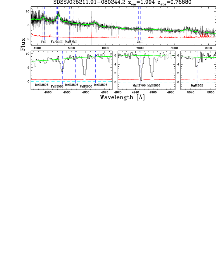
Figure 1: SDSS spectrum of QSO SDSSJ025211.91$-$080244.2 containing a strong Mg ii absorber at $z_{\rm abs}=0.7688$. The upper panel shows the entire spectrum (black histogram) with our PCA reconstruction of the QSO continuum (solid line). The error array is shown by the continuous line just above the zero flux level. The vertical dashed lines mark several transitions at the absorption redshift, including the Fe ii $\lambda 2600$ and the Mg i $\lambda 2852$ lines that we used to confirm the Mg ii doublet. These transitions are detailed in the lower panels. Detailed plots for all of our 1806 Mg ii absorbers can be viewed at http://www.ast.cam.ac.uk/$\sim$mim/pub.html.

The algorithm to select Mg ii absorbers from SDSS/DR3 differs in several ways from the algorithm used for SDSS/DR1 in Bouché et al. (2004), the most important of which is the method for estimating the QSO continuum. In Bouché et al. (2004) we used a series of overlapping polynomial fits to small Sections of the continuum. While this provides a reliable continuum in most cases, it does not perform well near sharp QSO emission lines, particularly when absorption lines – possibly the target Mg ii lines – are imprinted over the emission. To alleviate this problem in the current SDSS/DR3 analysis, we used principal component analysis (PCA) reconstructions of the QSO continua. Full details of the method are reported in Wild et al. (2006, see their appendix).

The features of the PCA algorithm most important for the present paper follow. Eigenspectra were generated in 4 QSO emission redshift bins to reduce the amount of data ‘missing’ due to the differing wavelength coverage of each spectrum: 0.005–0.458, 0.381–0.923, 0.822–1.537, 1.410–2.179, 2.172–3.193. An iterative procedure was used to identify and remove quasars showing broad absorption lines (BALs) during the creation of the PCA eigenspectra. This improves the continuum reconstruction of non-BAL quasar spectra, by removing from the input sample features which vary greatly in a small number of objects. Fig. 1 shows an example SDSS spectrum with its PCA continuum.

Having established a continuum, candidate Mg ii absorbers are identified as follows. We searched for intervening Mg ii absorbers from $\hbox{$z_{\rm abs}$}=0.37$ to $\hbox{$z_{\rm abs}$}=0.8$ (see Section 2.2). The low redshift cut arises from the fact that SDSS QSO spectra begin at $\approx$3800Å, and the high redshift cut was imposed since this is where LRGs drop below the SDSS magnitude limits. In addition, we require all Mg ii systems to be above the Ly$\alpha$ QSO emission line. QSOs above $\hbox{$z_{\rm em}$}=3.193$ are therefore not considered. All pixels above 1250 Å in the QSO rest-frame and $>3000\,\hbox{${\rm km\,s}^{-1}$}$ blue-wards of the MgII emission line are tested for Mg ii $\lambda 2796$ absorption. At each pixel, putative Mg ii $\lambda 2796$ lines are characterized using a method similar to that detailed by Schneider et al. (1993). For initial line detection, the rest-frame Mg ii $\lambda 2796$ equivalent width and 1-$\sigma$ detection limit are defined using the spectrograph instrumental profile (IP) as a weighting function and using pixels in a 7 Å window in the putative absorber’s rest-frame. The IP is assumed to be a Gaussian of width ${\rm FWHM}=160\,\hbox{${\rm km\,s}^{-1}$}$. If this estimate of the Mg ii $\lambda 2796$ equivalent width is $\geq 0.3$ Å and is significant at $\geq 8\,\sigma$ then the putative absorption redshift is estimated from a parabolic interpolation of the equivalent widths of the current pixel and its 2 neighbouring pixels. The equivalent width of the Mg ii $\lambda 2803$ line is estimated in a similar way based on the $\lambda 2796$ redshift. If the $\lambda 2803$ equivalent width is significant at $\geq 3\,\sigma$ then the system is flagged as a candidate Mg ii absorber. Spurious candidates are removed by visually inspecting each Mg ii candidate. The most common mis-identification is broad C iv absorption near the C iv emission line. Adopting a conservative approach, we rejected any candidates which did not show absorption in either Fe ii $\lambda 2600$ or Mg i $\lambda 2852$ at $\geq 1\,\sigma$ significance.

For each candidate we derive a refined estimate of the Mg ii $\lambda 2796$ equivalent width using a Gaussian fit to the absorption as a weighting function (c.f. the IP-weighting above). This new, somewhat more optimal, estimate is referred to throughout this paper as the measured Mg ii $\lambda 2796$ equivalent width, $W_{\rm r}^{\lambda 2796}$, for the system. Equivalent widths, with a similar Gaussian-fit weighting, are also derived for a variety of other commonly observed transitions (see Table 1).

With the above algorithm we detected and visually confirmed 1806 Mg ii absorbers in SDSS/DR3. Figure 2 (left panel) shows the distribution of the equivalent width of our Mg ii absorbers. Table 1 is an excerpt from the catalogue of absorbers which is available in its entirety in the electronic edition of this paper and from an on-line catalogue at http://www.ast.cam.ac.uk/$\sim$mim/pub.html. Figure 1 shows an example Mg ii absorption system. Similar plots are available for all absorption systems in the on-line catalogue.

Table 1: Catalogue of 1806 Mg ii absorbers from the SDSS DR3 with $0.37\!\leq\!z_{\rm abs}\!\leq\!0.80$. The J2000 name, QSO and absorption redshifts and the measured $W_{\rm r}$ for Mg ii$\lambda\lambda$2796 & 2803, Mg i $\lambda 2852$ and Fe ii $\lambda 2600$ are given. Here we show only a small sample from the full table which is available in the electronic edition of this paper and from http://www.ast.cam.ac.uk/$\sim$mim/pub.html. Full name designations, and statistical uncertainties in $W_{\rm r}$ are given in the electronic version, together with $W_{\rm r}$ measurements for the following transitions: Zn ii $\lambda\lambda$2026/2062, Cr ii $\lambda$2056/$\lambda$2062/$\lambda$2066, Fe ii $\lambda$2344/$\lambda$2374/$\lambda$2382/$\lambda$2586, Mn ii $\lambda$2576/$\lambda$2594/$\lambda$2606, Ti ii $\lambda$3242/$\lambda$3384, Ca ii $\lambda\lambda$3934/3969 and Na i $\lambda\lambda$5891/5897.

			Rest equivalent width $\left[{\rm\AA}\right]$
SDSSJ	$z_{\rm em}$	$z_{\rm abs}$	2796	2803	2852	2600
160530$+$393116	1.083	0.4969	1.04	0.79	0.04	0.19
160726$+$471251	1.816	0.4974	1.30	1.41	0.03	0.59
171726$+$654542	1.215	0.4974	3.29	3.39	0.22	1.39
112719$+$654143	1.250	0.4977	0.53	0.32	0.17	0.24

2.2 Luminous red galaxies

Figure 2: Left: Rest-frame equivalent width ($W_{\rm r}^{\lambda 2796}$) distribution of our 1806 Mg ii systems. Right: Redshift distribution of the LRGs (bottom) and Mg ii systems (top). The inset shows the distribution of QSO emission redshifts.

Eisenstein et al. ( 2001) (see also Scranton et al., 2003) presented colour criteria specifically designed to select luminous massive early types both locally and at $z>0.4$, i.e. much beyond the volume of the SDSS Main sample. Because of their association with luminous ($M_{r}\sim-21.5$), massive haloes and spectral uniformity, LRGs are excellent probes of the large scale structure as proven by the detection of the baryon oscillations by Eisenstein et al. ( 2005).

For each Mg ii absorber, galaxies meeting the following criteria (following Scranton et al., 2003) were extracted from the SDSS DR3 galaxy catalogue:

$$i^{*}_{\rm petro} < 21,$$ (1)

$$0.7(g^{*}-r^{*})+1.2[(r^{*}-i^{*})-0.18] > 1.6\,,$$ (2)

$$(g^{*}-r^{*}) > 1\,,$$ (3)

$$({\rm d}_{\perp}\equiv)(r^{*}-i^{*})-(g^{*}-r^{*})/8 > 0.4\,,$$ (4)

$$r^{*}_{\rm psf}-r^{*}_{\rm model} > 0.24\,,$$ (5)

$$\left|z_{\rm phot}-z_{\rm abs}\right| < 0.05\,.$$ (6)

We also required errors on the model magnitudes to be less than $0.2{\rm\,mag}$ in $r^{*}$ and $i^{*}$, and we excluded objects flagged by SDSS as BRIGHT, SATURATED, MAYBE_CR or EDGE. The model magnitudes, corrected for Galactic extinction, were used to compute the colours. Equations (1)–(4) are the LRG selection criteria of Scranton et al. (2003). Criterion (4) is equivalent to imposing $z_{\rm phot}\!\ga\!0.3$. Criterion (5) separates stars from galaxies. Criterion (6) is the selection of galaxies within a redshift slice of width $\Delta_{z}\!=\!0.1$ around $z_{\rm abs}$ using the photometric redshifts, $z_{\rm phot}$, of Csabai et al. (2003) who showed that these are accurate to $\sigma_{z}\!=\!0.1$.

The choice of the slice width $\Delta_{z}\!=\!0.1$ corresponds to $\sim\!200h^{-1}{\rm\,Mpc}$ (co-moving) and is arbitrary. We will show that the amplitude ratio between the absorber–galaxy cross-correlation and the galaxy–galaxy auto-correlation does not depend on the choice of $\Delta_{z}$ in Section 4.4 since we use the same redshift width for both correlation functions.

Finally, we remove the $\sim$10 per cent of galaxies with problematic photometric redshifts by requiring that galaxies have $z_{\rm phot}$ uncertainties $\sigma_{z}\!<\!0.5$. A total of 242,620 galaxies met all these criteria in our 1806 fields ($\sim\!800$ square degrees).

Figure 2(right) shows the redshift distribution of these LRGs for the 1806 fields. We used the spectroscopic redshift when available, which includes less than 1% of the sample. This small fraction is likely to increase in future with the joint 2dF/SDSS program to obtain spectra of LRGs (e.g. Padmanabhan et al., 2005).

3 Method

We first describe the basics of the galaxy clustering analysis in Section 3.1. The correlation estimator best used for this work is discussed in Section 3.2.

3.1 Galaxy clustering around QSO absorbers

A widely used statistic to measure the clustering of galaxies is the correlation function, $\xi(r)$. The absorber–galaxy cross-correlation, $\xi_{\rm ag}$, is defined from the conditional probability of finding a galaxy in a volume d$V$ at a distance $r=|\mathbf{r}_{2}\!-\!\mathbf{r}_{1}|$, given that there is a Mg ii absorber at $\mathbf{r}_{1}$:

$$P({\rm LRG}|\hbox{{\rm Mg}{\sc\,ii}})=\overline{n}_{u}\left[1+\xi_{\rm ag}(r)\right]\mathrm{d}V,$$ (7)

where $\overline{n}_{u}$ is the unconditional background galaxy density.

Because the observed amplitude of the auto- and cross-correlation functions are related to the dark matter correlation function, $\xi_{\rm DM}$, through the mean bias, $\overline{b}(M)$, which is a function of the dark matter halo-mass (e.g. Mo et al., 1993; Mo & White, 2002, and references therein),

$$\xi_{\rm gg}(r) = \overline{b}^{2}(M_{\rm g})\,\xi_{\rm DM}(r)\,,$$ (8)

$$\xi_{\rm ag}(r) = \overline{b}(M_{\rm a})\,\overline{b}(M_{\rm g})\,\xi_{\rm DM}(r)\,,$$ (9)

the relative amplitude of the cross-correlation will give a measurement of the bias ratio and thus of the relative halo-masses:

$$\frac{\xi_{\rm ag}}{\xi_{\rm gg}}=\frac{\overline{b}(M_{\rm a})}{\overline{b}(M_{\rm g})}\;.$$ (10)

In other words, if the amplitude of $\xi_{\rm ag}$ is greater (smaller) than $\xi_{\rm gg}$, the haloes of the absorbers are more (less) massive than those of the LRGs since the bias increases with halo mass in all hierarchical models.

In the remainder of this work, we will use only projected correlation functions, $w(r_{\theta})$, where $r_{\theta}=D_{A}(1+z)\theta$ for $D_{A}$ the angular diameter distance in co-moving Mpc. This is necessary since our sample is made up of absorbers with spectroscopic redshifts and of galaxies with photometric redshifts. The projected cross-correlation between Mg ii absorbers and LRGs, $w_{\rm ag}(r_{\theta})$, is related to $\xi_{\rm ag}(r)$ via $w_{\rm ag}(r_{\theta})=\int N(z)\xi_{\rm ag}(\sqrt{r_{\theta}^{2}+l^{2}})\,\mathrm{d}l$ where $N(z)\equiv\hbox{${\mathrm{d}N}/{\mathrm{d}l}$}$ is the line-of-sight distribution of LRGs and $l$ is the co-moving distance along the line of sight.

For galaxies distributed along the line of sight as a top–hat function of width $\Delta_{z}$ (normalized such that $\int\hbox{${\mathrm{d}N}/{\mathrm{d}l}$}\;\mathrm{d}l=1$), the amplitudes of both $w_{\rm gg}(r_{\theta})$ and $w_{\rm ag}(r_{\theta})$ are inversely proportional to $\Delta_{z}$ (see also Eisenstein, 2003; Bouché et al., 2005, appendix A):

$$w_{\rm gg}(r_{\theta}) = A_{\rm gg}\;r_{\theta}^{1-\gamma}\;\simeq\;r_{\theta}^{1-\gamma}\;r_{\rm 0,gg}^{\gamma}\;H_{\gamma}\times\frac{1}{\Delta_{z}}\,,$$ (11)

$$w_{\rm ag}(r_{\theta}) = A_{\rm ag}\;r_{\theta}^{1-\gamma}\;\simeq\;r_{\theta}^{1-\gamma}\;r_{\rm 0,ag}^{\gamma}\;H_{\gamma}\times\frac{1}{\Delta_{z}}\,,$$ (12)

where $H_{\gamma}=\hbox{$\frac{\Gamma(\frac{1}{2})\Gamma(\frac{\gamma-1}{2})}{\Gamma(\frac{\gamma}{2})}$}$ and $r_{\rm 0,gg}$ & $r_{\rm 0,ag}$ are, respectively, the galaxy–galaxy & absorber–galaxy correlation lengths. These two equations show that both $w_{\rm ag}$ and $w_{\rm gg}$ depend in exactly the same way on the width of the redshift distribution $\Delta_{z}$. Bouché et al. (2005, appendix A) showed that this is always true when one correlates one population with known redshifts (the Mg ii absorbers) with another population whose redshift is more uncertain. In Section 4.4, we will show empirically that the ratio $w_{\rm ag}/w_{\rm gg}$ is indeed independent of $\Delta_{z}$. Thus, we stress that $w_{\rm ag}/w_{\rm gg}$ is independent of the width of the LRG redshift distribution as long as one uses the same galaxies for $w_{\rm ag}$ and for $w_{\rm gg}$.

From equations (11) & (12), the ratio of the amplitudes of the two projected correlation functions,

$$a \equiv \frac{w_{\rm ag}}{w_{\rm gg}}\,,$$ (13)

is simply $(r_{\rm 0,ag}/r_{\rm 0,gg})^{\gamma}$, and is also equal to the bias-ratio $\overline{b}(M_{\rm\hbox{{\rm Mg}{\sc\,ii}}})/\overline{b}(M_{\rm LRG})$ [equation (10)] from which we infer the mean Mg ii halo-mass using the bias prescription of Mo & White (2002).

It is important to realise that measuring the halo-mass from the ratio of projected correlation functions has the following advantages, as advocated in Bouché et al. (2004) and Bouché et al. (2005): (i) one constrains the mass of the Mg ii host-galaxies in a statistical manner without directly identifying them, (ii) it is free of possible systematic errors due to foreground or background contaminants (i.e. stars or galaxies) and (iii) it does not require knowledge of the true width of the redshift distribution of the galaxy population. The first point is a natural consequence of correlation statistics. The last two points are consequences of the fact that the same galaxies are used to calculate $w_{\rm gg}(r_{\theta})$ and $w_{\rm ag}(r_{\theta})$ and that both $w_{\rm ag}$ and $w_{\rm gg}$ have the same dependence on the width of the galaxy redshift distribution [equations (11) & (12)]. This last point follows from the fact that the absorber redshift is known precisely (see Bouché et al., 2005, appendix A) as mentioned above. We will demonstrate points (ii) & (iii) empirically in Section 4.4.

Using smoothed particle hydrodynamical (SPH) simulations Bouché et al. (2005) showed that the measured amplitude ratio $w_{\rm ag}/w_{\rm gg}$ returns the bias-ratio $\overline{b}_{a}/\overline{b}_{g}$ that one expects given the known mass of the simulated galaxies. Specifically, the bias formalism of Mo & White (2002) predicts an amplitude ratio of 0.771 in the case of the DLA–galaxy cross-correlation – a situation very similar to the Mg ii–galaxy correlation considered here. Direct measurement of the correlation functions from the simulations yields $\overline{b}_{\rm DLA}/\overline{b}_{\rm gal}=0.73\pm 0.08$, in excellent agreement with the prediction. The simulations also demonstrated that the cross-correlation technique does not depend on the galaxy population used to trace the large scale structure and that foreground and background contaminants do not effect the measured bias-ratio.

3.2 Which correlation estimator to use?

Which estimator is best used to compute the Mg ii–LRG cross-correlation? For a given field (i.e. a single absorber), a seemingly natural choice would be the estimator

$$1+w_{\rm ag}(r_{\theta})=\frac{\rm G}{\rm R}\,,$$ (14)

where G is the observed number of galaxies between $r_{\theta}-dr/2$ and $r_{\theta}+\mathrm{d}r/2$ around the absorber, and $R$ is the number of absorber–random galaxy pairs normalized to the total number of galaxies in the field, $N_{\rm g}$, i.e. multiplied by $N_{\rm g}/N_{\rm r}$. Ideally, $R$ would simply be the area of the annulus times the surface density of galaxies. In practice, some fields are on the edges of the SDSS coverage, and the SDSS coverage itself is not completely uniform on the sky; there are small holes, areas missed by SDSS or not yet released. One overcomes these problems by (1) generating random galaxies excluding the gaps and edges, and (2) by generating $\sim 200$ times more random galaxies than real galaxies in order to reduce the shot noise in $R$ to an insignificant proportion.

In our case, we have 1806 fields, at relatively precise absorption redshifts, $z_{\rm abs}$. The selection function for the fields is therefore a sum of $\delta$-functions. Should one then use $\langle\frac{G}{R}\rangle$, where $\langle\rangle$ represents the averaging operator, in the right-hand side of equation (14)? This is clearly not optimum since it would treat each field equally in performing the average. Adelberger et al. (2003) (see their equation B3) showed that a better choice for the estimator of $w_{\rm ag}(r_{\theta})$ is $\langle G\rangle/\langle R\rangle$, i.e.:

$$1+{w}_{\rm ag}(r_{\theta})=\frac{\rm AG}{\rm AR}\,,$$ (15)

where AG $=\sum_{i}G_{i}$ is the observed number of absorber–galaxy pairs between $r_{\theta}-dr/2$ and $r_{\theta}+\mathrm{d}r/2$, summed over all the fields $i$. AR is the normalized number of absorber–random galaxy pairs. The normalization is applied to each field independently: ${\rm AR}\!=\!\sum_{i}{\rm R}^{i}\;N_{g}^{i}/N_{r}^{i}$, where Rⁱ is the number of random pairs in field $i$, and $N_{g}^{i}$ ($N_{r}^{i}$) is the total number of galaxies (random galaxies) for that field. Naturally, we took into account the areas missing from the survey within our search radius. Note each absorber’s redshift is used to compute $r_{\theta}$ from a pair separated by an angular separation $\theta$.

We stress that the Landy & Szalay (1993) estimator is not applicable here, since it is symmetric under the exchange of the two populations by one another. Here, the absorbers have spectroscopic redshifts, whereas the galaxies have photometric redshifts breaking the symmetry. Note that this asymmetry has an important consequence: it implies that both $w_{\rm ag}$ and $w_{\rm gg}$ have the same dependence on the galaxy redshift distribution, as indicated by equations (11) & (12) (see Bouché et al., 2005, appendix A).

The cross-correlation computed from equation (15) is biased low due to the integral constraint (e.g. Peebles, 1980), explained below. The reason for this is simply that the true correlation is defined as an overdensity with respect to the ‘unconditional’ galaxy density $\overline{n}_{u}$. This is not a measurable quantity as one uses the ‘observed’ galaxy density (or surface density $\Sigma_{g}$ for projected correlations) for the field over which one measures $w(r_{\theta})$. As a conseqence, the sum of all the pairs must be equal to the total number of galaxies $N_{g}$ observed in the survey of area $\Sigma$. This implies that the integral of $w_{\rm ag}$ over the area $\Sigma$ vanishes: $\int_{\Sigma}\;w_{\rm ag}\;\mathrm{d}\Sigma=0.$ To fulfill this condition, the cross-correlation $w_{\rm ag}$ will have to be $<0$ on the largest scales, i.e. biased low. This bias is refered to as the ‘integral constraint’, $C$. The true correlation function is then $w_{\rm ag}^{\rm C}={w}_{\rm ag}+C$, where $C$ is the integral constraint.

There are two ways to estimate $C$. Firstly, it can be estimated iteratively. For a given amplitude of the correlation, one can calculate the expected bias $C$ which is then used to correct the estimate of the amplitude. The second method is to fit $C$ when one has sufficient signal to noise. In the analysis below, we find that the first method gives $0.0217$, while the second gives $C=0.018\pm 0.012$ (keeping the other parameters fixed).

4 Results

In this Section, we first present the Mg ii–LRG cross-correlation (Section 4.1), and the LRG–LRG auto-correlation (Section 4.2) before showing the main result on the amplitude ratio between the Mg ii–LRG cross-correlation and LRG–LRG auto-correlation (Section 4.4). We turn the amplitude ratio into a halo-mass for the Mg ii absorbers in Section 4.5. Finally, we show that the amplitude ratio (or the halo-mass) varies with equivalent width in Section 4.6.

4.1 Mg ii–LRG cross-correlation

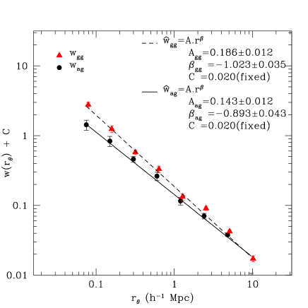
Figure 3: The filled circles show the projected Mg ii–LRG cross-correlation, $w_{\rm ag}(r_{\theta})$, for 1806 absorbers and $\sim$ 250,000 LRGs and the triangles show the LRG–LRG auto-correlation, $w_{\rm gg}(r_{\theta})$. The error bars are computed using the Jackknife technique. The independent fits to $w_{\rm ag}(r_{\theta})$ (solid line) and $w_{\rm gg}(r_{\theta})$ (dashed line) are shown. We fixed the integral constraint $C$ to 0.02 (see text).

Table 2: The total number of absorber–LRG pairs, AG, and the number of absorber–random pairs, AR, for the cross-correlation shown in Fig. 3.

$r_{\theta}$	AG	AR	$w_{\rm ag}$	$\sigma_{w}$
[$h^{-1}{\rm\,Mpc}$]
0.05–0.1	28	11.61	1.41	0.42
0.1–0.2	82	45.13	0.82	0.19
0.2–0.4	262	181.92	0.44	0.10
0.4–0.8	900	724.91	0.24	0.044
0.8–1.6	3183	2904.27	0.096	0.015
1.6–3.2	12205	11619.1	0.050	0.010
3.2–6.4	46867	46043.9	0.018	0.007
6.4–12.8	179093	181089	-0.011	0.002

Figure 3 (filled circles) shows the Mg ii–LRG cross-correlation for the entire sample of 1806 Mg ii absorbers, where we used equation (15) for the estimator of $w_{\rm ag}(r_{\theta})$. There are 242,620 objects within $r_{\theta}\!=\!12.8h^{-1}{\rm\,Mpc}$ which is the outer radius of the largest bin used. Table 2 shows the total number of pairs, AG, and the expected number of pairs, AR, if Mg ii absorbers and LRGs were not correlated. Figure 3 demonstrates that $w_{\rm ag}(r_{\theta})$ is a power-law at all scales. As a consequence, the dip at $\sim 100$ $h^{-1}$ kpc in the DR1 sample discussed in Bouché et al. (2004) appears to have been due to small number statistics.

The error bars for $w_{\rm ag}$ are computed using the jackknife estimator (Efron, 1982): we divide the sample into 10 parts and compute the covariance matrix from the $N_{\rm jack}\!=\!10$ realisations for each part:

$${\rm COV}_{ij}=\frac{N_{\rm jack}-1}{N_{\rm jack}}\sum_{k=1}^{N_{\rm jack}}[w_{k}(r_{\theta_{i}})-\overline{w}(r_{\theta_{i}})]\cdot[w_{k}(r_{\theta_{j}})-\overline{w}(r_{\theta_{j}})]$$ (16)

where $w_{k}$ is the $k$th measurement of the cross-correlation and $\overline{w}$ is the average of the $N_{\rm jack}$ measurements.

We fitted $w_{\rm ag}(r_{\theta})$ with a power law model, $\hat{w}_{\rm ag}(r_{\theta})=A_{\rm ag}\,r_{\theta}^{\beta_{\rm ag}}$, by minimizing

$$\chi^{2}\equiv\frac{1}{N_{\rm dof}}[\mathbf{w}-\mathbf{\hat{w}}]^{T}\mathrm{COV}^{-1}[\mathbf{w}-\mathbf{\hat{w}}]\,,$$ (17)

where $N_{\rm dof}$ is the number of degrees-of-freedom, $\mathbf{w}$ and $\mathbf{\hat{w}}$ are the vector data and model respectively, and ${\rm COV}^{-1}$ is the inverse of the covariance matrix. Since ${\rm COV}$ is singular we used singular value decomposition techniques to avoid instabilities in its inversion (see discussion in Bernstein, 1994). Since the integral constraint is $C=0.02\pm 0.01$ (see last Section), we add $\delta_{i,j}(0.01)^{2}$ to the covariance matrix ${\rm COV}(w)_{i,j}$ to form ${\rm COV}(w^{C})_{i,j}$, the covariance matrix for $w^{C}(r_{\theta})=w(r_{\theta})+C$.

Fitting the vector ${\mathbf{w}}^{C}$, the best-fit amplitude at $1h^{-1}{\rm\,Mpc}$ and power-law slope of the cross-correlation are, respectively,

$$A_{\rm ag} = \hbox{$0.143\pm 0.012$},$$

$$\beta_{\rm ag} = \hbox{$-0.893\pm 0.043$}.$$

Figure 4: The Mg ii-LRG cross-correlation amplitude as a function of the artificial redshift offset, $z_{\rm offset}$, imposed on the absorber redshifts. As expected, the cross-correlation signal vanishes when $|z_{\rm offset}|$ is increased. This shows that the cross-correlation signal in Fig. 3 is solely due to the Mg ii absorbers. The solid line represents a top-hat redshift distribution of width $\Delta_{z}=0.1$ convolved with a Lorentzian of width ${\rm FWHM}=0.176$, corresponding to the typical photometric redshift uncertainty of $\sigma_{z}=0.075$. The solid curve is scaled to the $z_{\rm offset}=0$ data point. The dotted line shows the solid line shifted by $z_{\rm shift}=-0.025$, representing the possible 5 per cent correction to the photometric redshifts suggested by Padmanabhan et al. (2005) (see text). The increase in the error-bars from left to right is due to the shape of the LRG redshift distribution in Fig. 2(right).

4.2 Luminous red galaxy auto-correlation

The LRG–LRG auto-correlation $w_{\rm gg}$ is represented by the grey/red triangles in Fig. 3. Since our goal is to measure the ratio $w_{\rm ag}/w_{\rm gg}$, we are forced to use the same estimator for $w_{\rm gg}$ as $w_{\rm ag}$, namely

$$1+\overline{w}_{\rm gg}(r_{\theta})=\frac{\rm GG}{\rm GR}\,,$$ (18)

where GG is the observed number of galaxy–galaxy pairs between $r_{\theta}-\mathrm{d}r/2$ and $r_{\theta}+\mathrm{d}r/2$ and GR is the number of galaxy–random galaxy pairs, computed as before. Again, $r_{\theta}$ is in units of co-moving Mpc. The errors and the covariance matrix for $w_{\rm gg}$ are computed using $N_{\rm jack}\!=\!10$ jackknife realisations, as before. Using the covariance matrix to $w_{\rm gg}^{C}$, ${\rm COV}(w^{C})_{i,j}$ (as in Section 4.1), we fitted a power-law, $\hat{w}_{\rm gg}(r_{\theta})=A_{\rm gg}\,r_{\theta}^{\beta_{\rm gg}},$ to $w_{\rm gg}(r_{\theta})$. The best-fit amplitude at $1h^{-1}{\rm\,Mpc}$ and the power-law slope are, respectively,

$$A_{\rm gg} = \hbox{$0.186\pm 0.012$},$$

$$\beta_{\rm gg} = \hbox{$-1.023\pm 0.035$}.$$ (19)

The conversion of the amplitude, $A_{\rm gg}$, to the co-moving correlation length, $r_{0,\rm gg}$, depends on having precise knowledge of the true redshift distribution, $N(z)$, of the LRG sample. The observed distribution is a convolution of the true distribution and the photometric redshift errors. Deconvolving these to find the true distribution is difficult (e.g. Padmanabhan et al., 2005) and is beyond the goal of this paper. However, we note that over a redshift range similar to ours ($z\!=\!0.3$–$0.9$), Brown et al. (2003) showed that red ($B_{W}\!-\!R\!>\!1.44$) galaxies in the NOAO deep wide survey have a correlation length of $r_{0}=6.3\pm 0.5h^{-1}{\rm\,Mpc}$, for galaxies in the luminosity range $-21.5\!<\!M_{R}\!<\!-20.5$. At the mean redshift of our sample, $z=0.5$, such clustering is consistent with halo-masses of $1\times 10^{13}$ M_⊙ using the bias prescription of Mo & White (2002). Brown et al. showed that the correlation length rapidly increases to $r_{0,\rm gg}=11.2h^{-1}{\rm\,Mpc}$ at $M_{R}\!=\!-22$. Our sample has a mean luminosity of $M_{r^{\star}}\simeq-21.5$, which is consistent with $r_{0,\rm gg}=8h^{-1}{\rm\,Mpc}$, and a halo-mass slightly higher: $M_{\rm LRG}=2$–$4\times 10^{13}$ M_⊙. Since we will see that the systematic errors in our final results are of the same order as the statistical errors, we hereafter assume that $M_{\rm LRG}=3\!\times\!10^{13}$ M_⊙ and treat the uncertainty in its value as an additional source of systematic errors. This is discussed further in Section 4.5.

4.3 Is the cross-correlation signal really due to the absorbers?

In order to verify that the signal of the cross-correlation is solely due to the Mg ii absorbers, we repeat our cross-correlation measurement adding an artificial offset $z_{\rm offset}$ to the absorber redshift $z_{\rm abs}$, with $z_{\rm offset}$ ranging from $-0.25$ to $+0.25$. Here, we fit the cross-correlation $w_{\rm ag}(r_{\theta})$ using the model $\hat{w}(r_{\theta})=A\;(r^{\beta}-0.02/0.15)$ in order to account for the fact that as $A$ tends to zero, so does the integral constraint $C$. The slope $\beta$ is kept fixed at $\beta=-0.89$.

Figure 4 shows the amplitude of the Mg ii–LRG cross-correlation $A_{\rm ag}$ as a function of the artificial redshift offset $z_{\rm offset}$. Because the amplitude vanishes when $|z_{\rm offset}|$ is increased, this figure shows that the Mg ii–LRG cross-correlation signal in Fig. 3 and in Bouché et al. (2004) is solely due to the Mg ii absorbers.

Given that Csabai et al. (2003) showed that the LRG photometric redshifts have a typical uncertainty of $\sigma_{z}\!=\!0.05$–$0.1$, we convolved our top-hat redshift selection function of width $\Delta_{z}=0.1$ with a Lorentzian with ${\rm FWHM}=2.35\,\sigma_{z}$, representing the typical photometric redshift uncertainty with an underlying population of ‘outliers’. The solid line in Fig. 4 shows the result of the convolution with $\sigma_{z}=0.075$. The data points in this figure might indicate that the photometric redshifts are slightly over-estimated. In fact, Padmanabhan et al. (2005) showed that at redshifts $z>0.4$, photometric redshifts are slightly over-estimated by 5 per cent, i.e. a redshift correction of $0.025$ at the mean redshift of our sample. The dotted line shows the shifted curve. We emphasize that this will not affect our results since we measure $w_{\rm ag}/w_{\rm gg}$, which has no dependence on the redshift distribution of the galaxies.

The error bars in Fig. 4 increase strongly with increasing $z_{\rm offset}$. This is due to our redshift selection function shown in Fig. 2: as a positive offset is added, far fewer galaxies are selected and the signal-to-noise ratio decreases since the number of galaxies directly drives the number of absorber-galaxy pairs.

4.4 The relative amplitude $\mn@boldsymbol{w_{\rm ag}/w_{\rm gg}}$

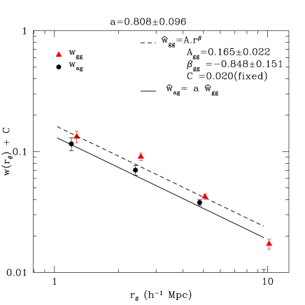
Figure 5: Same as in Fig. 3 in the two-halo regime $r_{\theta}>1$ $h^{-1}$ Mpc. The dashed line represents $\hat{w}_{\rm gg}$ and the relative amplitude of $w_{\rm ag}$ to $w_{\rm gg}$ (found using $\hat{w}_{\rm ag}=a\times\hat{w}_{\rm gg}$) is $a=\hbox{$0.808\pm 0.096$}$. From this, the bias-ratio $b_{\rm\hbox{{\rm Mg}{\sc\,ii}}}/b_{\rm LRG}$ is $\sim 0.65$ (see text), which in turn implies that Mg ii host-galaxies have haloes of mass $\hbox{$M_{\rm h}$}\!\simeq 10^{12}$ M_⊙ (see Section 4.5)

In order to measure the Mg ii–LRG bias-ratio [from equations (8) & (9)], one needs to use (i) the scales where the bias $b(M)$ dominates (i.e. where the correlation arises from 2 different haloes) and (ii) the same power-law slope, $\beta$, in order to compare the amplitudes of $w_{\rm ag}$ and $w_{\rm gg}$. The first point requires that we use only scales $r_{\theta}\!>\!1$ $h^{-1}$ Mpc, as numerous papers (both on simulations and on SDSS data) have shown that the correlations below these scales are dominated by the single-halo correlation between the central galaxy and its satellites (e.g. Berlind et al., 2003; Zehavi et al., 2004). The auto-correlation of $z=0$ SDSS galaxies shows a break at $1$ $h^{-1}$ Mpc where the transition between the single- and the two-halo terms occur. Point (ii) is easily achieved by using $\hat{w}_{\rm gg}$ (Section 4.2) as a template to constrain the relative amplitude of $w_{\rm ag}$:

$$\hat{w}_{\rm ag}=a\times\hat{w}_{\rm gg},$$ (20)

where $a$ is the amplitude ratio.

Figure 5 shows the auto- and cross-correlation on scales larger than $r_{\theta}\!>\!1$ $h^{-1}$ Mpc. We find that the best relative amplitude is

$$a=\hbox{$0.808\pm 0.096$}\,.$$ (21)

As we emphasized in Bouché et al. (2004) and pointed out in Section 4.1, the same galaxies are used to calculate $w_{\rm ag}$ and $w_{\rm gg}$. Therefore, the relative amplitude, $a$, is free of systematics from contaminants (stars or interloping galaxies). This is demonstrated in Fig. 6. The top panel shows $a$ as a function of the width $\Delta_{z}$ of the redshift slice. As one increases $\Delta_{z}$ up to $0.2$ ($\simeq 400$ Mpc), i.e. as one increases the number of foreground and background galaxies, the amplitude ratio is independent of that choice. The bottom panel shows that the amplitude of $w_{\rm ag}$, $A_{\rm ag}$, decreases with increasing redshift width, as one would expect [equation (12)]. However, $A_{\rm ag}$ does not follow the $1/\Delta_{z}$ behaviour predicted [Bouché et al. 2005 and equations (11) & (12)]. This is easily explained given that $\Delta_{z}$ is a selection criteria upon photometric redshifts: doubling $\Delta_{z}$ does not mean we doubled the width of the (true) redshift distribution since the finite uncertainty in the photometric redshifts, $\sigma_{z}$, is comparable to $\Delta_{z}$.

Figure 6: Top: Amplitude ratio $a$ [equivalently, the bias-ratio $\overline{b}(M_{\rm a})/\overline{b}(M_{\rm g})$] as a function of the width $\Delta_{z}$ of the redshift slice. The bias-ratio is independent of the redshift width selection. As a consequence, the ratio of the amplitude of the cross-correlation to that of the auto-correlation is free of systematics from contaminants (stars or interloping galaxies). Bottom: The amplitude $A_{\rm ag}$ of the cross-correlation $w_{\rm ag}$ decreases as the redshift slice selection increases, as expected. The vertical dashed line shows $\Delta_{z}=0.1$, the selection adopted here [equation (6)]. Both panels were computed in the $r_{\theta}>1$ Mpc regime as in Fig. 3.

As noted in Section 4.1, the bias-ratio $b_{\rm\hbox{{\rm Mg}{\sc\,ii}}}/b_{\rm LRG}$ is equal to $a$ in the case of a top-hat redshift distribution $N(z)$. However, given the uncertainties in the photometric redshifts, our LRG sample is distributed around the absorber redshifts in a Gaussian manner. In Bouché et al. (2004) and Bouché et al. (2005), we showed that, in the case of a Gaussian redshift distribution, the amplitude of the Mg ii–LRG cross-correlation relative to that of the LRG–LRG auto-correlation, $a$, is overestimated by $25\pm 10$ per cent. This correction factor was determined using (i) numerical integrations and (ii) mock catalogues (from the GIF2 collaboration, Gao et al., 2005) made of galaxies that had a redshift uncertainty equal to the slice width, $\Delta_{z}$, as in the case of our LRG sample. Thus, the bias-ratio inferred from the measured amplitude ratio equation (21)] is

$$\frac{\overline{b}_{\rm\hbox{{\rm Mg}{\sc\,ii}}}}{\overline{b}_{\rm LRGs}} = \hbox{$0.65\pm 0.08(\hbox{stat})\pm{0.05}(\hbox{sys})$}\,,$$ (22)

or $0.65\pm 0.09$ after adding the uncertainties in quadrature. For comparison, in Bouché et al. (2004), we used 212 Mg ii absorbers and $\sim\!20,000$ LRGs selected in SDSS/DR1 and found that the amplitude ratio was $0.67\pm 0.09$.

This bias measurement is entirely consistent with the results of Bergeron & Boissé (1991) and Steidel et al. (1994) who found that Mg ii absorbers with $\hbox{$W_{\rm r}^{\lambda 2796}$}\!\geq\!0.3$ Å are on average associated with late-type $\sim\!0.7L_{B}^{*}$ galaxies, since the expected amplitude ratio between early and late type galaxies is $\sim\!0.70$ (see Bouché et al., 2004). In addition, the auto-correlation of late-type galaxies has a shallower power-law slope than that of red early-type galaxies (e.g. Madgwick & et al.,, 2003; Collister & Lahav, 2005), a behaviour recovered in our cross-correlation $w_{\rm ag}$ measurement in Fig. 3.

4.5 Halo-masses of Mg ii absorbers

As already mentioned, in the context of hierarchical galaxy formation, equations (8) & (9) imply that equation (22) can be used to infer the halo-mass of the Mg ii absorbers provided that the mass of LRGs is known, which is the case here, as described in Section 4.2.

Figure 7: The solid line shows the bias $b(\hbox{$M_{\rm h}$})$ as a function of the halo-mass $\hbox{$M_{\rm h}$}(\hbox{M${}_{\odot}$})$ using the formalism of Mo & White (2002). The thick solid line shows the linear approximation over the mass range $\log\hbox{$M_{\rm h}$}\!=\!$ 11.8–13.2 used to estimate that our Mg ii absorbers have haloes with mass $\langle\log\hbox{$M_{\rm h}$}(\hbox{M${}_{\odot}$})\rangle=\;$$11.94^{+0.39}_{-0.40}$ [equation (24)] from the bias ratio [equation (22)]. The dotted line shows the linear approximation over the mass range $\log\hbox{$M_{\rm h}$}(\hbox{M${}_{\odot}$})\!=\!$ 10.7–13.5 used in Section 4.6. The inset zooms in on the region of interest.

However, the transformation of equation (22) into a halo-mass is not entirely straightforward. Indeed, as noted in Bouché et al. (2005), equations (8) & (9) refer to the mean bias, $\overline{b}$, averaged over the mass distributions $\overline{b}(>\!M)=\int_{M}^{\infty}p(M^{\prime})\,b(M^{\prime})\,\mathrm{d}\log M^{\prime}\,,$ where $p(M)\equiv\frac{\mathrm{d}n}{\mathrm{d}\log M}$ is the appropriate mass distribution [normalized such that $\int p(M)\,\mathrm{d}\log M=1$] and $b(M)$ is the bias of haloes of a given mass $M$, shown in Fig. 7. In the case of the LRGs, $p(M)$ is given by the halo mass function $n(M)$. Unfortunately, the distribution $p(M)\equiv{\mathrm{d}n}{/\mathrm{d}z/\mathrm{d}\log M}$ for the Mg ii absorbers is unknown.

As discussed in Bouché et al. (2005), this issue may be alleviated by expanding $b(M)$ to first order over a restricted mass range, i.e., $b(M)=b_{0}+b_{1}\;\log M$. The mean bias $\overline{b}$ is then given by

$$\overline{b}(>\!M_{\rm min}) = \int_{M_{\rm min}}^{\infty}p(M^{\prime})\,b(M^{\prime})\,\mathrm{d}\log M^{\prime}$$ (23)

$$= b_{0}+b_{1}\,\int_{M_{\rm min}}^{\infty}p(M^{\prime})\,\log M^{\prime}\,\mathrm{d}\log M^{\prime}$$

$$= b_{0}+b_{1}\,\langle\log M\rangle\,,$$

where $\langle\log M\rangle$ is the first moment of the distribution $p(M)$. For example, the mean bias of the Mg ii absorbers is $\overline{b}$ evaluated at the mean halo-mass, i.e. $\overline{b}_{\rm\hbox{{\rm Mg}{\sc\,ii}}}=\overline{b}(\langle\log\hbox{$M_{\rm h}$}\rangle)$, where $<>$ is the average using the appropriate mass distribution $p(M)$. Since the coefficients $b_{0}$ & $b_{1}$ can be obtained from the bias function $b(M)$, the distribution $p(M)$ need not to be known.

The thick dashed line in Fig. 7 shows the linear fit to $b(M)$ over $\sim 1.4$ dex. Provided that the mass range of interest is small ($\la 1$ dex), this approximation is valid. Using this linear fit to $b(M)$, our bias-ratio measurement equation (22) implies that the Mg ii absorbers reside in haloes of mean mass

$$\langle\log\hbox{$M_{\rm h}$}(\hbox{M${}_{\odot}$})\rangle=\hbox{$11.94\pm{0.31}(\hbox{stat})^{+0.20}_{-0.19}$ (\hbox{sys})},$$

regardless of the actual $p(M)$ distributions. An additional source of systematic error is the mass of LRGs, which has been assumed to be $\sim\!3\!\times\!10^{13}$ M_⊙. Given that the uncertainty in the correlation length $r_{0,\rm gg}$ is of the order of $\sim\!1$ Mpc at most (Section 4.2), we find that the uncertainty in the LRG halo-mass is ${}^{+0.21}_{-0.25}$ dex. This implies that the additional systematic uncertainty in the absorber halo-mass is ${}^{+0.14}_{-0.16}$ dex.

By adding this additional systematic uncertainty in quadrature, we find that the mean halo-mass of Mg ii absorbers is (with 1-$\sigma$ uncertainties):

$$\langle\log\hbox{$M_{\rm h}$}(\hbox{M${}_{\odot}$})\rangle=\hbox{$11.94\pm{0.31}(\hbox{stat})^{+0.24}_{-0.25}$ (\hbox{sys})}\,.$$ (24)

Adding the statistical and systematic errors in quadrature gives $\langle\log\hbox{$M_{\rm h}$}(\hbox{M${}_{\odot}$})\rangle=\hbox{$11.94^{+0.39}_{-0.40}$}$.

Is this mass scale $\sim\!10^{12}$ M_⊙ consistent with the incidence probability of Mg ii absorbers? In other words, are there too many (or too few) such haloes in a $\Lambda$CDM universe? The incidence probability of Mg ii absorbers, ${\mathrm{d}N}/{\mathrm{d}z}$, is given by the volume number-density of haloes, $n$, times the co-moving cross-section, $\sigma_{\rm co}$:

$$\frac{\mathrm{d}N}{\mathrm{d}z}\;=\;n\,\sigma_{\rm co}\,\frac{\mathrm{d}r}{\mathrm{d}z}\,,$$ (25)

where the cross-section $\sigma_{\rm co}=\pi R_{\rm phys}^{2}(1+z_{\rm abs})^{2}$ for $R_{\rm phys}$ the radius of the cross-section in physical units. Since $R_{\rm phys}$ is $\sim$40 $h^{-1}$ kpc (Steidel, 1995) and the number density of haloes of mass $M=10^{12}$ M_⊙ is $n=10^{-2}h^{-3}$ Mpc^-3 (Mo & White, 2002), we find that $\hbox{${\mathrm{d}N}/{\mathrm{d}z}$}\simeq 0.3\;(n/10^{-2})\;(R_{\rm phys}/40\,\hbox{\hbox{$h^{-1}$~{}kpc}})^{2}$. This is close to the observed value for Mg ii absorbers with $\hbox{$W_{\rm r}^{\lambda 2796}$}\ga 1$ Å (Nestor et al., 2005; Prochter et al., 2005). We can therefore conclude that there are neither too few nor too many $\hbox{$M_{\rm h}$}=10^{12}$ M_⊙ haloes to account for the observed incidence probability.

4.6 Are $\mn@boldsymbol{W_{\rm r}}$ and $\mn@boldsymbol{M_{\rm h}}$ anti-correlated?

Table 3: The bias-ratio and the inferred halo-mass of Mg ii absorbers, with 1-$\sigma$ statistical uncertainties, as a function of $W_{\rm r}^{\lambda 2796}$, binned in two different ways. The first splits the sample of nabstot Mg ii absorbers into 4 bins of equal size except for the last bin which is double the size to provide enough statistics. The second uses 3 bins of equal size. Regardless of the binning, the bias-ratio decreases with increasing $W_{\rm r}^{\lambda 2796}$.

$W_{\rm r}^{\lambda 2796}$(Å)	$a\equiv w_{\rm ag}/w_{\rm gg}$	$b_{\rm\hbox{{\rm Mg}{\sc\,ii}}}/b_{\rm LRG}$	$\log M_{\hbox{{\rm Mg}{\sc\,ii}}}(\hbox{M${}_{\odot}$})$
0.3–5.5	$0.808\pm 0.096$	$0.65\pm 0.08$	$11.94\pm{0.31}$
0.30–1.15	0.99 $\pm$ 0.11	0.79 $\pm$ 0.09	$12.49\pm 0.34$
1.15–2.00	0.81 $\pm$ 0.11	0.65 $\pm$ 0.08	$11.93\pm 0.33$
2.00–2.85	0.54 $\pm$ 0.17	0.43 $\pm$ 0.13	$11.11^{+0.52}$
2.85–5.50	0.66 $\pm$ 0.24	0.53 $\pm$ 0.19	$11.47^{+0.74}$
0.725–1.575	1.13 $\pm$ 0.12	0.89 $\pm$ 0.09	$12.88\pm 0.37$
1.575–2.415	0.70 $\pm$ 0.13	0.56 $\pm$ 0.11	$11.59\pm 0.41$
2.415–4.115	0.61 $\pm$ 0.14	0.49 $\pm$ 0.11	$11.30\pm 0.43$

Figure 8: Left: The bias-ratio $b(M_{\rm a})/b(M_{\rm g})$ as a function of rest-frame equivalent width $W_{\rm r}^{\lambda 2796}$ using 3 equally spaced bins plus a larger bin. The bias-ratio is computed from the ratio of the Mg ii-LRG cross-correlation to the LRG-LRG auto-correlation measured on scales $1$–13 $h^{-1}$ Mpc as in Section 4.4. The bias-ratio is anti-correlated with $W_{\rm r}^{\lambda 2796}$. This anti-correlation implies that higher equivalent width absorbers are less massive. Right: The halo-mass, $\hbox{$M_{\rm h}$}(\hbox{M${}_{\odot}$})$, of Mg ii absorbers as a function of $W_{\rm r}^{\lambda 2796}$ in bins corresponding to those on the left plot. Absorbers with $\hbox{$W_{\rm r}^{\lambda 2796}$}\!\ga\!1.5$ Å have a halo-mass 1 dex smaller than absorbers with $0.3\!\la\!\hbox{$W_{\rm r}^{\lambda 2796}$}\!\la\!1.0$ Å.

We searched for possible correlations between the halo-masses of our 1806 Mg ii absorbers and various parameters of our survey such as the absorber redshift $z_{\rm abs}$, the quasar redshift $z_{\rm qso}$, Mg ii equivalent width, signal-to-noise of the SDSS spectra, $W_{\rm r}^{\lambda 2796}$, the quasar magnitude and the quasar colours. We did not find any significant correlation with these parameters except for the equivalent width, $W_{\rm r}^{\lambda 2796}$. Our DR1 sample (Bouché et al., 2004) already showed tentative evidence that the cross-correlation had a slightly smaller amplitude for higher equivalent width absorbers. Here we significantly strengthen that evidence.

Figure 8(left) shows the bias-ratio $b_{\rm\hbox{{\rm Mg}{\sc\,ii}}}/b_{\rm LRG}$ for sub-samples in 4 equivalent width bins of equal width except for the last bin which is twice as large in order to have enough statistics. This figure shows that the bias-ratio, and therefore the halo-mass, is anti-correlated with $W_{\rm r}^{\lambda 2796}$. We also divided our sample into 3 sub-samples of 602 absorbers. Table 3 lists the halo-masses for each $W_{\rm r}^{\lambda 2796}$ bin and shows that the anti-correlation is robust under different binning. The bias-ratio in this figure is computed from the ratio of the Mg ii–LRG cross-correlation to the LRG–LRG auto-correlation measured on large scales ($1$–13 $h^{-1}$ Mpc) as in Section 4.4. In other words, the anti-correlation shown in Fig. 8 has nothing to do with ‘Mg ii absorbers in the haloes of LRGs’, since the haloes of LRGs are much smaller than the scales probed by our clustering.

Figure 8(right) shows the halo-mass inferred for each of the 4 bins used in the left plot. In converting bias-ratio to halo-mass, we used the same method outlined in Section 4.5. However, since the bias-ratio in Fig. 8(left) corresponds to a larger mass range than in Section 4.5, we adopted the dotted line shown in Fig. 7 as a linear approximation to the bias function [equation (23)]. This approximation is naturally poorer than for our mass estimate for the entire sample [equation (24)]. Of course, equation (23) can be expanded to the second order, but it would include the second moment $\langle(\log M)^{2}\rangle$ of the distribution $p(M)$, which is unknown. Quantitatively, we find that absorbers with $W_{\rm r}^{\hbox{$\lambda 2796$}}\ga 2$ Å have haloes with $\langle\log M_{h}(\hbox{M${}_{\odot}$})\rangle=\;$$11.3^{+0.4}_{-0.4}$, while Mg ii absorbers with $0.3\!\la\!\hbox{$W_{\rm r}^{\lambda 2796}$}\!\la 1.0$ Å have $\langle\log M_{h}(\hbox{M${}_{\odot}$})\rangle=\;$$12.5_{-0.3}^{+0.3}$, i.e. a mass difference of $\ga$1.0 dex.

The observed $M_{\rm h}$–$W_{\rm r}^{\lambda 2796}$ anti-correlation in Fig. 8 has important implications. If Mg ii clouds were virialized entities in the gaseous haloes of the host-galaxies, one would expect that the velocity spread of Mg ii systems would be proportional to the mass of the host galaxies. At equivalent widths $\hbox{$W_{\rm r}^{\lambda 2796}$}\!\geq\!0.3$ Å, the Mg ii transitions of the sub-components are saturated and so $W_{\rm r}^{\lambda 2796}$ strongly correlates with the velocity spread ($\Delta v$) of the absorber (e.g. Ellison, 2006). This velocity range for strong Mg ii systems covers the range 50–400 ${\rm km\,s}^{-1}$. If the individual clouds are virialized in the halo of the host-galaxies, $\Delta v$ ought to be related to the velocity dispersion of the gaseous halo and to the mass of the host galaxy. Therefore, the $M_{\rm h}$–$W_{\rm r}^{\lambda 2796}$ anti-correlation shows that most strong Mg ii absorbers are not virialized in the gaseous haloes of their host-galaxies.

In fact, it is often tacitly assumed in the literature that $M_{\rm h}$ and $\Delta v$ (as traced by $W_{\rm r}^{\lambda 2796}$) should be positively correlated and so the $M_{\rm h}$–$W_{\rm r}^{\lambda 2796}$ anti-correlation in Fig. 8 may seem surprising at first. In the next Section, we show that this auto-correlation is compatible with numerous past results in the literature. Moreover, those past results actually seem to require a $M_{\rm h}$–$W_{\rm r}^{\lambda 2796}$ anti-correlation, independent of our new results.

Recently, Prochter et al. (2005) used the redshift evolution of ${\mathrm{d}N}/{\mathrm{d}z}$ and simple cross-section arguments to infer rough estimates of the halo-mass of Mg ii absorbers. Their conclusions are similar to ours: absorbers with large equivalent width, $\hbox{$W_{\rm r}^{\lambda 2796}$}\ga 1.8$ Å, were found to be more likely associated with $\hbox{$M_{\rm h}$}<M_{\star}$ haloes, not with massive $M_{\star}\sim 10^{12}$ M_⊙ haloes.

5 Do past results require a $M_{\rm h}$–$W_{\rm r}^{\lambda 2796}$ anti-correlation?

In this Section, we study the incidence probability of absorbers in more detail. Specifically, we use two arguments to show that a $M_{\rm h}$–$W_{\rm r}^{\lambda 2796}$ anti-correlation is already required by past results, i.e. regardless of our cross-correlation results. In Section 5.1, we show that the cross-section–luminosity relationship combined with the cross-section–equivalent width relationship require an anti-correlation between luminosity and equivalent width. In Section 5.2, we show that the cross-section–luminosity relationship, the observed incident probability ($\mathrm{d}^{2}N/\mathrm{d}z/\mathrm{d}W_{\rm r}$) and any plausible host-galaxy luminosity function (LF) together require an anti-correlation between luminosity and equivalent width. We also show that the slope of the expected anti-correlation is completely consistent with our new result in Fig. 8.

The starting point for the discussions below is the incidence equation, equation (25), but in its integral form:

$$\int_{W_{1}}^{W_{2}}\frac{\mathrm{d}^{2}N}{\mathrm{d}W_{\rm r}\mathrm{d}z}(W_{\rm r})\mathrm{d}W_{\rm r}$$ (26)

$$= \int_{M_{1}}^{M_{2}}\mathrm{d}\log M\,\frac{\mathrm{d}^{2}N}{\mathrm{d}\log M\mathrm{d}z}(M)$$

$$= \int_{M_{1}}^{M_{2}}\mathrm{d}\log M\,\frac{\mathrm{d}^{2}N}{\mathrm{d}\log M\mathrm{d}V}(M)\,\sigma_{\rm co}(M)\,\frac{\mathrm{d}r}{\mathrm{d}z}\,,$$

where ${\mathrm{d}^{2}N}/{\mathrm{d}\log\!M/\mathrm{d}V}$ is the number of haloes (or galaxies) per unit volume per unit mass (or luminosity). In addition, a covering factor $C_{\rm f}$ should be included in the right-hand side of this equation since observations imply that it may be less than unity: Tripp & Bowen (2005) studied close galaxy–QSO pairs and found that $\sim$50 per cent of galaxies do not produce any Mg ii absorption down to 0.3 Å, indicating that the mean covering factor for our sample is $C_{\rm f}\sim 0.5$. We note that $C_{\rm f}$ is likely to depend on the size of the host galaxy and therefore its mass, a complication that we ignore here.

For the past two decades, the main problem in solving equation (26) for the cross-section $\sigma_{\rm co}$ was that one had to perform the integrals of the left-hand side over a range of $W_{\rm r}^{\lambda 2796}$ and the right-hand side over a range of mass $M$ (or luminosity $L$), ignoring any possible – and probably quite strong – dependence of $W_{\rm r}^{\lambda 2796}$ on $L$ or $M$. We will show in the next two sub-sections that the $M_{\rm h}$–$W_{\rm r}^{\lambda 2796}$ anti-correlation is required (independently of our cross-correlation results).

We first show (in Section 5.1) that a $M_{\rm h}$–$W_{\rm r}^{\lambda 2796}$ relationship is required from the following simple arguments. Observationally, for a given bin in $W_{\rm r}^{\lambda 2796}$, there is a maximum impact parameter, $R_{\rm phys}$, that defines the cross-section, $\sigma$. The radius of the cross-section depends on the luminosity of the host galaxy, $R_{\rm phys}\propto L^{\beta}$, i.e. the cross-section is a function of mass or luminosity. Since there is a relationship between $W_{\rm r}^{\lambda 2796}$ and $R_{\rm phys}$ and between $R_{\rm phys}$ and $L$, there is a relationship between $W_{\rm r}^{\lambda 2796}$ and $M_{\rm h}$ (or $L$). Section 5.1 shows that the two physical parameters should be anti-correlated. Section 5.2 arrives at the same conclusion based on different arguments which make one assumption, namely that the relationship between $\log\hbox{$M_{\rm h}$}$ and $W_{\rm r}^{\lambda 2796}$ is linear.

5.1 The cross-section distributions require a $M_{\rm h}$–$W_{\rm r}^{\lambda 2796}$ anti-correlation

Figure 9: The Mg ii equivalent width, $W_{\rm r}^{\lambda 2796}$, as a function of impact parameter, $\rho$, for the host-galaxies of absorbers with $\hbox{$W_{\rm r}^{\lambda 2796}$}\ga 0.3$ Å. The solid squares show the impact parameters for host-galaxies selected from a sample of our SDSS Mg ii absorbers closer than 100$h^{-1}$ kpc (co-moving) to the QSO lines-of-sight and with $|z_{\rm phot}-z_{\rm abs}|<0.05$. The open squares, open triangles and solid triangle show the samples of Steidel (1995), Kacprzak et al. (2006) and Bergeron & Boissé (1991) respectively. All impact parameters are shown in our cosmology. The solid line shows the fiducial model for the maximum impact parameter $R_{\rm phys}$ used in Section 5.1 (see text) to represent the cross-section–equivalent width relationship, $\sigma_{\rm co}(\hbox{$W_{\rm r}^{\lambda 2796}$})$.

Here, we investigate the existence of a luminosity (or mass)–$W_{\rm r}^{\lambda 2796}$ relationship and whether the two parameters should be correlated or anti-correlated given the observed distribution of Mg ii absorbers in the cross-section–equivalent width plane and the dependence of the cross-section on luminosity (Steidel, 1995).

The radius of the cross-section, $R_{\rm phys}$, decreases steeply with increasing $W_{\rm r}^{\lambda 2796}$: Lanzetta & Bowen (1990) and Steidel (1995) (their figure 3) showed that the host-galaxies of absorbers with $\hbox{$W_{\rm r}^{\lambda 2796}$}>2$ Å do not exist at large impact parameters. Figure 9 reproduces these results. The data points show the impact parameters $\rho$ (in physical units) of the Mg ii host galaxies from the samples of Bergeron & Boissé (1991) (filled triangle), Steidel (1995) (open squares) and Kacprzak et al. (2006) (open triangles) for absorbers with $\hbox{$W_{\rm r}^{\lambda 2796}$}>0.3$ Å. The solid squares represent the 44 host-galaxies that we have identified in the SDSS/DR3 imaging data with $|z_{\rm abs}-z_{\rm phot}|<0.05$ and which were within 100 kpc (co-moving) of the QSO line-of-sight. This sample is truncated at an impact parameter $\rho\la 20$ $h^{-1}$ kpc (physical; $\sim$3″) due to the large point-spread function of SDSS. It is clear that the data points do not fill the upper right side of the plot. More precisely, at increasing equivalent width, the maximum impact parameter – which defines the radius $R_{\rm phys}$ of the cross-section – decreases. This dependence can be roughly parametrized as $W_{\rm r}(R_{\rm phys})\simeq-3\log[R_{\rm phys}]+K$ as represented by the solid line in Fig. 9.

In addition, a relationship between between $R_{\rm phys}$ and luminosity $L$ also exists: Steidel (1995) found that $R_{\rm phys}$ slightly increases with luminosity: $R_{\rm phys}(L)\propto(L_{K}/L_{K}^{*})^{\beta}$, with $\beta\simeq 0.2$. Thus, the simple observational results that there are relationships between $W_{\rm r}$ & $R_{\rm phys}$ and between $R_{\rm phys}$ & $L$ require a $L$–$W_{\rm r}^{\lambda 2796}$ relationship.

We emphasize that this $L$–$W_{\rm r}^{\lambda 2796}$ relationship does not mean that there is a direct correspondence between mass and equivalent width on a galaxy-by-galaxy basis. This relationship simply means that on average a sample with a well-defined $W_{\rm r}^{\lambda 2796}$ (e.g. a bin of $W_{\rm r}^{\lambda 2796}$) will have a well-defined and predictable mean mass (or luminosity). More specifically, for a sample of absorbers selected in a bin of $W_{\rm r}^{\lambda 2796}$, the host galaxy will have an impact parameter less than $R_{\rm phys}$, and a mean mass $M_{\rm h}$. One should not interpret the distribution in $W_{\rm r}^{\lambda 2796}$ as being entirely due to the distribution in halo mass (or in galaxy luminosity).

Finally, if one combines the observed cross-section–equivalent width relation (Fig. 9) with this cross-section–luminosity relation one finds that $W_{\rm r}^{\rm phys}(\log L_{K})\propto-3\beta\log L_{K}\simeq-0.6\log L_{K}$, i.e. $\log L_{K}\propto\frac{1}{-3\beta}W_{\rm r}\simeq-1.6W_{\rm r}$. In other words, the cross-section as a function of luminosity and as a function of equivalent width together require that $W_{\rm r}$ (therefore $\Delta v$) and luminosity (or mass) be anti-correlated.

5.2 The incidence probability requires a $M_{\rm h}$–$W_{\rm r}^{\lambda 2796}$ anti-correlation

Figure 10: The symbols represent the absorber $K$-band luminosity function (LF) of Steidel (1995). The error bars are uniform and represent the average uncertainties. The solid line represents a Schechter function with $\alpha=-1$, as observed for the field $K$-band LF (Kochanek et al., 2001). The dashed line represents a Schechter function with $\alpha=-0.5$. Both lines are reasonable descriptions of the $K$-band LF. Both curves were scaled to match the data points.

Since we have established the existence of a $M_{\rm h}$–$W_{\rm r}^{\lambda 2796}$ relationship, the right-hand side of equation (26) can be rewritten as

$$\int_{W_{1}}^{W_{2}}\mathrm{d}W_{\rm r}\frac{\mathrm{d}\log M}{\mathrm{d}W_{\rm r}}\,\frac{\mathrm{d}^{2}N}{\mathrm{d}\log M\mathrm{d}V}\,\sigma_{\rm co}\,\frac{\mathrm{d}r}{\mathrm{d}z}\,.$$

By differentiation of both sides of equation (26), it follows that 

$$\frac{\mathrm{d}^{2}N}{\mathrm{d}W_{\rm r}\mathrm{d}z} = \frac{\mathrm{d}\log M}{\mathrm{d}W_{\rm r}}\,\frac{\mathrm{d}^{2}N}{\mathrm{d}\log M\mathrm{d}V}\,\sigma_{\rm co}\,\frac{\mathrm{d}r}{\mathrm{d}z}\,,$$ (27)

where $\frac{\mathrm{d}\log M}{\mathrm{d}W_{\rm r}}$ is the Jacobian of the transformation between $W_{\rm r}$ and $M$. We will assume that the relationship between $W_{\rm r}$ and $M$ is linear, i.e. $\frac{\mathrm{d}\log M}{\mathrm{d}W_{\rm r}}$ is a constant.

An independent way to show the existence of a $L$–$W_{\rm r}$ anti-correlation makes use of equation (27) in terms of luminosity:

$$\frac{\mathrm{d}^{2}N}{\mathrm{d}z\mathrm{d}W_{\rm r}} = \frac{\mathrm{d}\log L}{\mathrm{d}W_{\rm r}}\,\frac{\mathrm{d}^{2}N}{\mathrm{d}V\mathrm{d}\log L}\;\sigma_{\rm co}(L)\;\frac{\rm dr}{\rm dz}\,,$$ (28)

where ${\mathrm{d}^{2}N}/{\mathrm{d}V/\mathrm{d}\log\!L}$ is simply the LF in logarithmic form, $\phi(L)L\ln(10)$. The differential incidence probability, $\mathrm{d}^{2}N/\mathrm{d}z/\mathrm{d}W_{\rm r}$, is now well constrained observationally thanks to the large SDSS database (e.g. Nestor et al., 2005; Prochter et al., 2005).

For luminosities below $L_{*}$, $\phi(L)L\propto L^{1+\alpha}$, where $\alpha$ is the faint-end power-law slope of the LF. Equation (28) then implies that

$$\frac{\mathrm{d}^{2}N}{\mathrm{d}z\mathrm{d}\log L} \propto L^{(1+\alpha+2\beta)}\,$$ (29)

using $\sigma_{\rm co}(L)\propto L^{2\beta}$ from Steidel (1995). In addition, Nestor et al. (2005) showed that $\mathrm{d}^{2}N/\mathrm{d}z/\mathrm{d}W_{\rm r}$ is an exponential, i.e.

$$\frac{\mathrm{d}^{2}N}{\mathrm{d}z\mathrm{d}W_{\rm r}} \propto \exp(-W_{\rm r}/W_{*})\,,$$ (30)

where $W_{*}$ is the exponential scale length.

Quantitatively, from equations (29) and (30), the expected slope of the $L$–$W_{\rm r}$ anti-correlation is

$$\frac{\rm d\log L}{\rm dW_{\rm r}} \simeq \frac{-\log_{10}(e)/W^{*}}{1+\alpha+2\beta},$$

$$\simeq -1.8\;\hbox{for $\alpha=-1.0$, or}$$

$$\simeq -0.8\;\hbox{for $\alpha=-0.5$},$$

since Nestor et al. (2005) showed that $W^{*}\sim 0.6$ in the redshift range $\langle z\rangle\sim 0.5$ of our survey, and Steidel (1995) showed that $\beta=0.2$ .

Therefore, equations (29) and (30) imply that $W_{\rm r}$ and $\log L$ (or $\log M$, using a constant $M/L$) must be anti-correlated as long as ${1+\alpha+2\beta}>0$, i.e. $\alpha>-1.4$ for $\beta=0.2$. Most plausible LFs easily satisfy this condition.

The $B$-band LF of Mg ii absorbers was constrained by Steidel et al. (1995) and is known to be bell-shaped, with $\alpha$ shallower than $-1$ (figure 4 of Steidel, 1995). The $K$-band LF of Mg ii is likely to be closer to a mass function. Figure 10 reproduces the absorber $K$-band luminosity function of Steidel (1995). The error bars are uniform and represent the average uncertainties. The solid line represents a Schechter function with $\alpha=-1$, as observed for the $z=0$ $K$-band field-galaxy LF (Kochanek et al., 2001; Bell et al., 2003). Steidel (1995) argued that the host-galaxy $K$-band luminosity function is similar to the $K$-band field-galaxy LF. The dashed line represents a Schechter function with $\alpha=-0.5$ and is an equally good match to the data.

One can go a step further and ‘predict’ the $M_{\rm h}$–$W_{\rm r}^{\lambda 2796}$ relationship using the mass-to-light ratio. Since the faint-end slope of the mass function of haloes (e.g. Mo & White, 2002) is steeper than that of galaxies, the halo mass-to-light ratio, $\hbox{$M_{\rm h}$}/L$, decreases with increasing $L$ (see Shankar et al., 2006, and references therein). Parametrizing $\hbox{$M_{\rm h}$}/L$ as $L^{q}$ (with $q\la 0$), one finds that the expected slope of the $M_{\rm h}$–$W_{\rm r}^{\lambda 2796}$ relationship is:

$$\frac{\rm d\log M}{\rm dW_{\rm r}} = (1+q)\frac{\rm d\log L}{\rm dW_{\rm r}}$$ (32)

$$\simeq (1+q)\frac{-\log_{10}(e)/W^{*}}{1+\alpha+2\beta}$$

Fig. 11(left) plots the expected relationship between $M_{\rm h}$ and $W_{\rm r}^{\lambda 2796}$ for $q=0,-0.5$ & $-0.75$ and $\alpha=-1.0$ & $-0.5$, with all curves normalized at $\log\hbox{$M_{\rm h}$}(\hbox{M${}_{\odot}$})=12$. The data points are as in Fig. 8(right) and agree well with the expected relationships (lines).

Figure 11: Left: The black squares show the halo-mass ($M_{\rm h}$) as a function of equivalent width ($W_{\rm r}^{\lambda 2796}$) as in Fig. 8(right). The grey squares show a different binning. The various lines represent the expected $M_{\rm h}$–$W_{\rm r}^{\lambda 2796}$ relationship, normalized at $\log\hbox{$M_{\rm h}$}(\hbox{M${}_{\odot}$})=12$, for various LFs ($\alpha=-1.0,-0.5$) and mass-to-light ratios ($q=0,-0.5,-0.75$) [see text and equation (32)]. The results from our cross-correlation analysis follow the expected anti-correlation. The error bars represent the 1-$\sigma$ statistical uncertainties and the size of the equivalent width bin used. Right: $W_{\rm r}^{\lambda 2796}$ as a function of impact parameter, $\rho$, for the Mg ii host-galaxies. The data points are as in Fig. 9. The lines are as in the left panel and represent the radii of the cross-section $R_{\rm phys}$ (i.e. maximum impact parameter allowed). The numbers along the dot-dash line indicate the logarithm of the halo mass corresponding to the $W_{\rm r}^{\lambda 2796}$ from the left panel.

Our conclusion from this exercise is that any plausible LF, combined with $\mathrm{d}^{2}N/\mathrm{d}z/\mathrm{d}W_{\rm r}$ (e.g Nestor et al., 2005) and with the observed $R_{\rm phys}(L_{K})$ relation (Steidel, 1995), together require a $L$–$W_{\rm r}^{\lambda 2796}$ (or $M_{\rm h}$–$W_{\rm r}^{\lambda 2796}$) anti-correlation.

Since a $M_{\rm h}$–$W_{\rm r}^{\lambda 2796}$ anti-correlation is required from past results, we can perform a simple consistency check as follows. We use the series of relationships shown in Fig. 11(left) and the halo-mass function, $n(\hbox{$M_{\rm h}$})\equiv{\mathrm{d}N}/{\mathrm{d}V}/{\mathrm{d}\log M}$, from Mo & White (2002) in equation (27) to predict the radius $R_{\rm phys}$ of the cross-section as a function of equivalent width, $R_{\rm phys}(\hbox{$W_{\rm r}^{\lambda 2796}$})$, that is required by the incidence distribution $\mathrm{d}^{2}N/\mathrm{d}z/\mathrm{d}W_{\rm r}$ of Nestor et al. (2005). The result is shown in Fig. 11(right) for each of the relationships on the left plot. The data points are as in Fig. 9.

Thus, we have shown with two different arguments (in Sections 5.1 & 5.2) that a positive $M_{\rm h}$–$W_{\rm r}^{\lambda 2796}$ correlation is not consistent with the impact parameter distribution ($\rho$–$W_{\rm r}^{\lambda 2796}$) of current Mg ii samples. This conclusion is completely independent of our clustering results presented in Section 4. One can turn these arguments around and state that the anti-correlation between $W_{\rm r}^{\lambda 2796}$ and maximum impact parameter (Fig. 9) is a natural outcome of the $M_{\rm h}$–$W_{\rm r}^{\lambda 2796}$ anti-correlation in Fig. 8.

6 Physical Interpretation

The $M_{\rm h}$–$W_{\rm r}^{\lambda 2796}$ anti-correlation has a direct and important consequence: As described in the introduction, if the individual sub-components or clouds of strong Mg ii systems were virialized within the host-galaxy halo, the velocity spread $\Delta v$ (as traced by $W_{\rm r}^{\lambda 2796}$) would be a measure of the galaxy velocity dispersion and would be correlated with $M_{\rm h}$  via $\hbox{$W_{\rm r}^{\lambda 2796}$}/\hbox{$\lambda 2796$}=\Delta v/c$ (or with the circular velocity of the galaxy, $V_{c}$, via $\hbox{$W_{\rm r}^{\lambda 2796}$}/\hbox{$\lambda 2796$}=V_{c}/c$). However, as demonstrated in Sections 5.1 and 5.2, one would not reproduce the observed relation between $R_{\rm phys}$ and $W_{\rm r}^{\lambda 2796}$. Thus, both our cross-correlation results and the arguments presented in Section 5 show that the Mg ii clouds are not virialized in the gaseous haloes of the host-galaxies, in the sense that the velocity spread $\Delta v$ (as traced by $W_{\rm r}^{\lambda 2796}$) of the sub-components is not proportional to halo mass.

We now turn towards a physical interpretation of our results. In particular, can we put constraints on the competing models for Mg ii absorbers?

6.1 Basic Mg ii cloud properties

In a few cases the physical properties (sizes, densities etc.) of the individual components of Mg ii systems with $\hbox{$W_{\rm r}^{\lambda 2796}$}>0.3$ Å have been constrained from photo-ionization modelling. For instance, Ding et al. (2003) and Masiero et al. (2005) found that individual Mg ii velocity components (or clouds) of systems with $\hbox{$W_{\rm r}^{\lambda 2796}$}>0.3$ Å have gas densities of $n_{\rm H}=0.001$–$0.1{\rm\,cm}^{-3}$ and, therefore, typical sizes of $s=10$–$1000{\rm\,pc}$, close to the direct size measurements of Rauch et al. (2002) using lensed QSOs. For a warm ($T\!\sim\!10^{4}$ K) cloud of size $s\!=\!100$ pc and $n_{\rm H}=0.01$ cm^-3, the sound crossing time is $\sim\!10^{7}$ yr, and the cooling time-scale is $k\,T/[n\Lambda(T)]\sim 10^{6}$ yr since the cooling function $\Lambda(T)\simeq 10^{-22}$ erg cm³ s^-1 at $T=10^{4}$ K (Sutherland & Dopita, 1993). The same ionization studies indicate that the associated Mg i components are denser ($n_{\rm H}\ga$10 cm^-3) but very small, only $0.01$–$0.1$ pc. This supports the view in which the clouds would condense out of the hot gas.

For such warm clouds embedded in a hot ($T\sim 10^{6}$ K) ionized medium, the evaporation time scale is $>\!10^{7}$ yr (Cowie & McKee, 1977; McKee & Cowie, 1977). They are stable against gravity because their Jeans lengths are much larger than the cloud sizes, but they would be destroyed by shocks in $s/v_{\rm shock}$$\sim 1$ Myr for a shock velocity $v_{\rm shock}$ of 100 ${\rm km\,s}^{-1}$ (Klein et al., 1994).

6.2 HVCs and Mg ii clouds

The properties of the Galactic high-velocity clouds (HVCs) – their H i column densities, sizes, densities etc. – are akin to those of Lyman limit and Mg ii absorbers (e.g. Charlton et al., 2000; Zwaan & Briggs, 2000). For instance, Richter et al. (2005) studied the Galactic gaseous halo in high-resolution spectra towards one line-of-sight (PKS 1448$-$232) and detected low column density, high-velocity Ca ii ($N_{\rm CaII}\sim 10^{11\hbox{--}12}$ cm^-2) and Na i D ($N_{\rm NaI}\sim 10^{11}$ cm^-2) absorption at $v_{\rm LSR}\simeq-150$ ${\rm km\,s}^{-1}$ with Doppler widths of 4–8 ${\rm km\,s}^{-1}$. This is very similar to typical values for Mg ii absorbers (Churchill et al., 2003). Their follow-up VLA 21-cm studies unveiled several high-velocity H i clumps at peak column densities $\hbox{$N_{\rm HI}$}\sim 10^{19}$ cm^-2 near the QSO line-of-sight. The sight-line seems to have intercepted the outer part of one of the clumps. Assuming a distance of 4–12 $h^{-1}$ kpc, the density of this clump is $n_{\rm H}\simeq 0.1$ cm^-3, similar to that inferred for Mg ii clouds by Ding et al. (2003). Because 8 of 13 sight-lines have similar high-velocity Ca ii clouds, Richter et al. (2005) concluded that the covering factor of such low column density gas must be large. Based on this they argued that if such clumps are typical for haloes of quiescent spiral galaxies, such low column density clouds should contribute significantly to the population of Mg ii absorbers and Lyman limit systems. In a starburst environment these clouds may be either more numerous and/or have larger column densities.

Towards the Andromeda galaxy (M31), Thilker et al. (2004) reported a population of faint H i clouds detected directly with the Green Bank Telescope (GBT). Follow-up studies by Westmeier et al. (2005) using the Westerbork telescope clearly show that the clouds have typical sizes of $\sim 1$ kpc, H i column densities of $10^{19\hbox{--}20}$ cm^-2, densities $n_{\rm H}\sim 10^{-2}$ cm^-3, H i line widths of $\sim\!20$ ${\rm km\,s}^{-1}$ and velocity gradients of several ${\rm km\,s}^{-1}$. The H i mass of these clouds is then $\sim 3\times 10^{5}$ M_⊙. Thus, the properties of HVCs are very close to those inferred for Mg ii clouds from photo-ionization studies discussed in Section 6.1 (see also the recent analysis of Fox et al., 2005).

6.3 Finding the right model

There are three main hypotheses that could describe Mg ii absorbers. The first assumes that QSO sight-lines probe galactic gaseous disks and, therefore, the interstellar medium of the host-galaxies. The second assumes that each QSO sight-line probes gaseous haloes of galaxies where the gas originates from the filaments, falls into the galactic potential well and eventually cools onto a rotationally supported disk. The third hypothesis places the Mg ii absorbing gas in the same gaseous halo, but the gas comes from outflows driven by the large number of supernovae in star-bursts. This last hypothesis has long been used to model the HVCs in the context of a ‘galactic fountain’ scenario in a multi-phase medium (e.g. Shapiro & Field, 1976; Wolfire et al., 1995).

The disk model predicts a strong dependence of $W_{\rm r}^{\lambda 2796}$ on inclination of the disk with respect to the line-of-sight. Kacprzak et al. (2005, 2006) did not find any such correlation. Furthermore, Steidel et al. (2002) found that, in a small sample of 5 Mg ii absorbers, an extension of the host-galaxy rotation curve did not reproduce the absorption-line kinematics. A simple disk model therefore seems unlikely.

The evolution of the Mg ii incidence probability is observed to strongly mimic the evolution of the star formation rate density (SFRD) with redshift, as pointed out by Prochter et al. (2005) and also Misawa et al. (2005). Indeed, removing the cosmological dependence (i.e. $\mathrm{d}r/\mathrm{d}z$) from the incidence probability, ${\mathrm{d}N}/{\mathrm{d}z}$, in equation (27) leads to the line-density of absorbers per co-moving Mpc, ${\mathrm{d}N}/{\mathrm{d}X}\equiv n(M)\,\sigma_{\rm co}$. This line-density shows a decline at $z<1$, just like the SFRD, and both ${\mathrm{d}N}/{\mathrm{d}X}$ and the SFRD are approximately constant from $z\sim 3$ to $z=1$. The decline of ${\mathrm{d}N}/{\mathrm{d}X}$ can only be explained by a decrease in the cross-section, $\sigma_{\rm co}$, with time since the number density of haloes, $n(M)$, increases with time for all masses. From these arguments, Prochter et al. (2005) concluded that “the processes responsible for strong Mg ii absorbers are turning off at $z\sim 1$”. This behaviour is natural within a starburst scenario where Mg ii absorbers are directly related to supernovae-driven winds.

Regarding the in-fall hypothesis, Mo & Miralda-Escudé (1996) produced a model for Lyman limit systems, Mg ii and C iv absorbers in a CDM cosmology. This model consists of a two phase medium for the gaseous halo. In the context of galaxy formation in dark matter haloes (e.g. White & Rees, 1978; White & Frenk, 1991), the initial gas in a galaxy (either at the time of collapse or through accretion) is shocked at around the virial radius. A halo of hot gas ($T\!\sim\!10^{6}$ K) is formed which has a temperature close to the halo virial temperature since it is in an approximate hydrostatic equilibrium with the dark matter. Due to cooling from thermal instabilities and inhomogeneities, a warm phase ($T\!\sim\!10^{4}$ K) will form, comprising photo-ionized clouds confined by the pressure of the hot phase, while accreting onto the galactic central region.

As a consequence, in this inflow picture the photo-ionized clouds will be approximately virialized in the gaseous halo. Mo & Miralda-Escudé (1996) argued that the terminal velocity of these clouds will be close to the virial velocity for haloes with $V_{c}<250$ ${\rm km\,s}^{-1}$. In this scenario, the velocity spread of the gas $\Delta v$ (as measured by $W_{\rm r}^{\lambda 2796}$) would be related to the virial velocity and therefore its halo-mass. Thus, we view the observed $M_{\rm h}$–$W_{\rm r}^{\lambda 2796}$ anti-correlation as strong evidence against this inflow picture. Furthermore, more massive (and larger) galaxies with large $W_{\rm r}^{\lambda 2796}$ would be seen at large impact parameters, contrary to the observations of Lanzetta & Bowen (1990) and Steidel et al. (1995).

There is one main caveat to this conclusion. The in-fall model of Mo & Miralda-Escudé (1996) might not be directly relevant to our absorbers with $\hbox{$W_{\rm r}^{\lambda 2796}$}\!\sim\!1$–$4$ Å which are expected to be optically thick, i.e. saturated. The in-fall model assumes the clouds are optically thin, i.e. $\hbox{$W_{\rm r}^{\lambda 2796}$}\la 0.3$ Å, still on the linear part of the curve of growth. Most such absorbers are predicted to be in massive galaxies, with a median $V_{c}=220$ ${\rm km\,s}^{-1}$ [$\log\hbox{$M_{\rm h}$}(\hbox{M${}_{\odot}$})\sim{12.4}$] and most systems in the range $V_{c}=150$–$300$ ${\rm km\,s}^{-1}$ [$\log\hbox{$M_{\rm h}$}(\hbox{M${}_{\odot}$})\sim 11.9$–$12.8$]. This mass range, predicted for $W_{\rm r}^{\lambda 2796}$$\simeq 0.3$ Å absorbers, agrees with our mass estimates for the lowest $W_{\rm r}^{\lambda 2796}$ systems in our sample (0.3–1.0 Å). The inflow model could therefore describe Mg ii absorbers with $\hbox{$W_{\rm r}^{\lambda 2796}$}\la 0.3$ Å. We also note that the $W_{\rm r}^{\lambda 2796}$ distribution function has different power-law indexes below and above 0.3 Å (Nestor et al., 2005), possibly reflecting two different physical origins.

Another possible caveat is the recent realisation that, for low mass galaxies, a significant fraction of the gas accretion occurs without the initial shock heating because the cooling time is very short, i.e. the gas remains warm ($T\sim 10^{4}$ K) as it moves from the intergalactic medium to the central parts of galaxies. For this reason, it is often referred to as the ‘cold mode’ of gas accretion (e.g. Birnboim & Dekel, 2003; Kereš et al., 2005). In this context, the clouds will not be virialized, but the terminal velocity should still be related to the halo-mass.

Maller & Bullock (2004) extended the arguments of Mo & Miralda-Escudé (1996) to include multi-phase cooling since the hot gas in galactic haloes is thermally unstable (see also discussion in Section 6.1). This multi-phase cooling scenario allows the survival of a hot gas core and naturally gives rise to the formation of $\sim\!10^{4}$ K clouds, each of mass $\sim 10^{6}$ M_⊙, which are pressure-confined by the hot halo. The main conclusion of this model relevant to our work is that this multi-phase treatment naturally explains the properties of Mg ii clouds and HVCs: the unstable hot gas produces warm clouds of mass $\sim\!10^{6}$ M_⊙ which are stabilized by the pressure of the surrounding hot gas. In this model, the maximum distance or impact parameter for warm clouds (HVCs) is set by the the ‘cooling radius’, which is $\sim\!100$ kpc for a Milky Way size halo. This model differs from the one of Sternberg et al. (2002) in that the self-gravity plays a negligible role and no dark matter is required.

Sternberg et al. (2002) modelled the HVCs as multi-phase (warm-ionized and cold-neutral) pressure-confined cloud, each belonging to a ‘mini-halo’ made of dark matter. In this model, the dark matter in the mini-haloes provide the extra pressure in the core of the clouds required to allow for the formation of a cold medium. The warm phase of the HVCs is confined by the ambient pressure provided by the hot ($T\!\sim\!10^{6}$ K) ionized gas of the halo. This hot gas is in hydro-static equilibrium with the dark-matter of the host galaxy and determines the pressure profile of a galaxy. Given the observed velocity widths (10–20 ${\rm km\,s}^{-1}$), Sternberg et al. (2002) determined that the pressure of this hot-gas must be $P/k>50$ cm^-3 K to keep the warm phase of the clouds bound. In the Milky Way, the pressure of the hot halo is above $50$ cm^-3 K out to 150–200 $h^{-1}$ kpc, i.e. almost to the virial radius. For galaxies with smaller halo-mass (or smaller virial temperature), the central pressure will be reduced and the radius at which $P/k$ reaches 50 cm^-3 K will be smaller than the virial radius, at which point the cloud will evaporate.

The fact that no absorbers with large $W_{\rm r}^{\lambda 2796}$ are found to have host-galaxies at large impact-parameters (i.e. no points to the right of the solid line in Fig. 9) clearly tells us something about the characteristic scale where clouds either form or evaporate, and not the size of the halo of the host-galaxy. Indeed, for the halo-masses found in Fig. 11(left) one can compare the corresponding virial radii to the $\rho$–$W_{\rm r}^{\lambda 2796}$ distribution in Fig. 11(right), as we show in Figure 12. The dashed line represents the $z=0.5$ virial radius, $r_{200}$, for the model with $\alpha=-0.75$ and $q=0$ in Fig. 11(left). The logarithm of the halo-masses (in M_⊙) are marked along the solid line. The halo circular velocity, $V_{c}$, is marked along the dashed line in ${\rm km\,s}^{-1}$. This figure clearly shows that $r_{200}$ is much larger than the cross-section radius ($R_{\rm phys}$, solid line) for absorbers with $\hbox{$W_{\rm r}^{\lambda 2796}$}\!>\!1.5$ Å (or halo-masses $M_{h}\!<10^{11.5}$ M_⊙). In other words, Mg ii absorbers do not fill the halo of the host-galaxy. The radius of the cross-section must then be due to some other physical mechanism. It could be either the pressure threshold discussed by Sternberg et al. (2002) and/or to the cooling radius of Maller & Bullock (2004).

Figure 12: Equivalent width, $W_{\rm r}^{\lambda 2796}$, as a function of impact parameter, $\rho$, as in Fig. 11(right). The data points are as in Figs. 9 & 11(right). The solid line shows one of the model curves from Fig. 11, the long dashed line. The numbers along the solid line indicate the logarithm of the halo mass in units of M_⊙) corresponding to the equivalent width. The dashed line shows the virial radius of such haloes ($r_{200}$), with the corresponding virial velocity marked. The virial radius is much greater than the cross-section radius, $R_{\rm phys}$, for absorbers with $\hbox{$W_{\rm r}^{\lambda 2796}$}\!>\!1.5$ Å. Therefore, strong Mg ii absorbers seem not to fill the haloes of their host-galaxies.

6.4 In the context of super-winds

Local supernovae-driven winds are known to expel ionized gas into their haloes, as traced by H$\alpha$, X-rays and certain emission lines (e.g. Lehnert & Heckman, 1994; Heckman et al., 1995; Armus et al., 1995; Lehnert & Heckman, 1996; Wang et al., 1997; Dahlem et al., 1997). However, the presence of Na i D absorption also indicates that the winds carry large amounts of dust and cold gas, $M\ga 10^{8}\hbox{M${}_{\odot}$}$, over the life-time of the star-burst (e.g. Lehnert & Heckman, 1996; Martin, 1999; Heckman et al., 2000; Rupke et al., 2005; Martin, 2006). The dust can sometimes be seen in direct imaging (Howk & Savage, 2000) out to a few kpc. Furthermore, the amount of dust is correlated with the amount of cold gas traced by Na i D absorption (Heckman et al., 2000; Martin, 2006). This shows that cold material is entrained and expelled outside the disk by the ionized gas flow. In this context, the findings of Kondo et al. (2006), York et al. (2006) and Wild, Hewett & Pettini (2006) are very interesting. For the first time, Kondo et al. detected strong Na i D$\lambda\lambda$5891/5897 doublet absorption in two strong Mg ii absorbers (also DLAs) at $\hbox{$z_{\rm abs}$}=1.062$ & $1.18$ towards the gravitationally lensed QSO APM 08279$+$5255. York et al. (2006) constrained the dust-reddening from the slope of stacked QSO spectra with foreground Mg ii absorbers selected similarly to ours, but at $1\!<\!\hbox{$z_{\rm abs}$}\!<\!1.8$. Finally, Wild & Hewett (2005) and Wild et al. (2006) found that the sub-sample of strong Mg ii absorbers showing significant Ca ii absorption in the low-resolution SDSS QSO spectra are even more dust-reddened. Both York et al. and Wild et al. found that the reddening is correlated with equivalent width, a relationship very similar to that of Heckman et al. (2000).

The metallicity of our Mg ii systems is unknown but York et al. used indirect arguments to estimate average metallicities for a DR1 sample of Mg ii absorbers. They found that the metallicity decreases with increasing Mg ii equivalent width. This would lead to a normal mass–metallicity relation when combined with our $M_{\rm h}$–$W_{\rm r}^{\lambda 2796}$ anti-correlation.

Given these local results and that Mg ii absorbers predominantly trace clouds of ‘cold’ material, are the Mg ii clouds related to the entrained material in outflows  ? If so, then $W_{\rm r}^{\lambda 2796}$ should be a measure of the (past) star-formation rate and mass ejection history for the following reasons. Firstly, $W_{\rm r}^{\lambda 2796}$ is a measure of the number of components (or clouds), as shown by Churchill et al. (2003). Secondly, our results show that absorbers with $\hbox{$W_{\rm r}^{\lambda 2796}$}\ga 2$ Å have smaller potential wells so the host-galaxy’s supernovae-driven winds are more likely to eject gaseous material out of the disks. Thus, in the context of galactic outflows, the velocity spread (and therefore $W_{\rm r}^{\lambda 2796}$), which is just a measure of the number of components, is related to the (past) star-formation rate and to the mass ejection rate.

Entrained clouds would have to survive from the disk to where they are seen at $R\sim 50$ kpc. The travel time to 50 kpc is about 100 Myr for wind speeds of 500 ${\rm km\,s}^{-1}$. From the discussion in Section 6.1, the formation and destruction time-scales are 1–2 orders of magnitude smaller than the travel time or halo dynamical time ($\simeq$ 0.5–1 Gyr). It seems very unlikely that such clouds could survive several times 100 Myr given these physical properties unless they are confined by the pressure of the hot ionized medium. The same conclusion was reached by Sternberg et al. (2002) and Maller & Bullock (2004) and is discussed above.

Recently, Kacprzak et al. (2005, 2006) reported that the host-galaxy morphological asymmetry and $W_{\rm r}^{\lambda 2796}$ are correlated. While these authors favour the merger interpretation for their results, they also discuss the possibility of star-burst driven winds. Again, because of the smaller potential wells of higher $W_{\rm r}^{\lambda 2796}$ absorbers, outflows driven by spatially asymmetric star-bursts can create asymmetries and produce the correlation seen by Kacprzak et al. (2005, 2006) without invoking mergers. In fact, one sees that most Mg ii host-galaxies in their sample are relatively isolated and do not show galaxy pairs or strongly disturbed morphologies.

6.5 Further evidences for the super-wind scenario

Direct evidence of outflows exists in only a few Mg ii absorbers. Bond et al. (2001) presented high-resolution spectra of four strong ($\hbox{$W_{\rm r}^{\lambda 2796}$}\!>\!1.8$ Å) Mg ii absorbers at $1\!<\!z\!<\!2$ and showed that the profiles “display a common kinematic structure, having a sharp drop in optical depth near the centre of the profile and strong, black-bottomed absorption on either side”. They interpret these features as a signature of super-winds arising in actively star-forming galaxies. In the similar case of the $z=0.74$ Mg ii host-galaxy towards QSO Q1331+17 (Ellison et al., 2003), the absorber’s absolute luminosity is quite low, $L\sim 0.3L^{*}$, and the authors suggest that “the double-peaked absorption profiles, their striking symmetries, … and large Mg ii equivalent width support the interpretation of superbubbles”.

Norman et al. (1996) searched for Mg ii absorption in QSO spectra that lie near the starburst galaxy NGC 520, a well-known local starburst with super-winds. NGC 520 has an IR-luminosity comparable to that of M82, shows a disturbed morphology and strong filamentary H$\alpha$ emission along the minor axis. In Norman et al., the Mg ii, Mg i, and Fe ii absorption associated with its gaseous halo are clearly detected along two lines-of-sight. The QSOs Q0121+0338 and Q0121+0327 intersect the halo of NGC 520 at $\sim\!55$ $h^{-1}$ kpc and $\sim\!25$ $h^{-1}$ kpc, respectively. In both sight-lines, the Mg ii equivalent widths are greater than $0.3$ Å: $\hbox{$W_{\rm r}^{\lambda 2796}$}=0.33$ Å towards Q0121+0338 and $\hbox{$W_{\rm r}^{\lambda 2796}$}=1.7$ Å towards Q0121+0327. The latter absorber with the largest $W_{\rm r}^{\lambda 2796}$ has the smallest impact parameter, as expected from the larger sample in Fig. 9.

7 Summary

From the SDSS/DR3 we selected 1806 Mg ii absorbers with $\hbox{$W_{\rm r}^{\lambda 2796}$}\!\geq\!0.3$ Å in the redshift range $0.4\!\leq\!\hbox{$z_{\rm abs}$}\!\leq\!0.8$ and $\sim$ 250,000 LRGs in the absorber fields selected with photometric redshifts. From the ratio of the Mg ii–LRG cross-correlation to the LRG–LRG auto-correlation, we constrained the halo-mass of Mg ii absorbers in a statistical manner, i.e. without directly identifying them. To summarise our main results, we have shown that:

1. the ratio of the cross- and auto-correlation, $w_{\rm ag}/w_{\rm gg}$, is $a=\hbox{$0.808\pm 0.096$}$;

2. the corresponding bias-ratio between strong Mg ii absorbers and LRGs is $b_{\rm\hbox{{\rm Mg}{\sc\,ii}}}/b_{\rm LRG}=\hbox{$0.65\pm 0.08$}$;

3. this bias-ratio implies that the absorber host-galaxies have a halo-mass of $\langle\log\hbox{$M_{\rm h}$}(\hbox{M${}_{\odot}$})\rangle=\;$$11.94^{+0.39}_{-0.40}$. The 1-$\sigma$ uncertainty includes the statistical errors in $a$ and possible systematic errors in the LRG halo-mass;

4. the Mg ii equivalent width, $W_{\rm r}^{\lambda 2796}$, is significantly anti-correlated with the absorber halo-mass, $M_{\rm h}$.

The main consequence of point (iv) is that the Mg ii clouds are not virialized in the gaseous haloes of the host-galaxy, in the sense that $\Delta v$, the velocity spread of the individual clouds (ranging from 50 to $\sim~{}400$ ${\rm km\,s}^{-1}$), does not positively correlate with halo mass. In other words, had the clouds been in virial equilibrium with the halo dark matter distribution, $\Delta v$ (as measured by $W_{\rm r}^{\lambda 2796}$) would correlate with the mass of the halo. However, we find the opposite: lower-mass haloes harbour the host-galaxies producing the largest number of individual Mg ii clouds spread over the largest velocities.

Since the $M_{\rm h}$–$W_{\rm r}^{\lambda 2796}$ anti-correlation may initially seem surprising, we performed several consistency tests on the method itself and tested the $M_{\rm h}$–$W_{\rm r}^{\lambda 2796}$ anti-correlation against numerous past results in the literature. For the galaxy clustering method we have shown that:

• The cross-correlation is solely due to the Mg ii absorbers;

• The cross-correlation amplitude decreases when the width of the LRG redshift distribution is increased, as expected;

• The $w_{\rm ag}/w_{\rm gg}$ ratio is independent of the LRG redshift distribution, as expected if one uses the same galaxies to calculate both $w_{\rm ag}$ and $w_{\rm gg}$. Therefore, the relative amplitude is free of possible systematic errors caused by contaminants (stars or interloping galaxies).

In checking past results in the literature for consistency with the observed $M_{\rm h}$–$W_{\rm r}^{\lambda 2796}$ anti-correlation we found that:

• When one combines the observed luminosity- and $W_{\rm r}^{\lambda 2796}$-dependence of the cross-section, one finds that luminosity (or mass) and equivalent width must be anti-correlated;

• When one combines the observed luminosity-dependence of the cross-section with the observed incidence probability of strong Mg ii absorbers, $\mathrm{d}^{2}N/\mathrm{d}z/\mathrm{d}W_{\rm r}$, one finds that luminosity (or mass) and equivalent width must be anti-correlated for all plausible luminosity functions with faint-end power-law indexes $\alpha>-1.4$.

In other words, a positive correlation between $W_{\rm r}^{\lambda 2796}$ and halo-mass (or virial velocity) – expected if the clouds were virialized – is inconsistent with past results. This is independent of the $M_{\rm h}$–$W_{\rm r}^{\lambda 2796}$ anti-correlation from the clustering analysis. When one combines the observed $M_{\rm h}$–$W_{\rm r}^{\lambda 2796}$ relationship with the observed $\mathrm{d}^{2}N/\mathrm{d}z/\mathrm{d}W_{\rm r}$ one predicts a cross-section radius which agrees very well with the distribution of absorber impact parameters observed in previous and current samples.

We interpret our results as a strong indication that a large proportion of strong Mg ii absorbers, particularly those with $\hbox{$W_{\rm r}^{\lambda 2796}$}\ga 2$ Å, arise in galactic outflows. A conclusion similar was reached by Songaila (2006) for $z\sim 2$ C iv absorbers. Supernovae-driven winds drive hot gas out of the galaxy plane, forming cavities if numerous supernova explosions occur in a small region on a similar time-scale. The hot gas breaks out of the disk, forming a hot gaseous corona (traced by high-ions such as C iv and O vi) and may entrain cold, dusty material. Part of this gas cools, forming pressure-confined clouds traced by Mg ii which may be the analogs of the HVCs.

This interpretation allows us to make several predictions. Firstly, it provides a natural explanation as to why absorbers with $\hbox{$W_{\rm r}^{\lambda 2796}$}>2$ Å are not observed at large impact parameters. These systems should be physically closer to the host galaxy and also closer in time to more recent and more active star formation. Thus, they ought to have star formation rates typical of star-bursts. The resonance line O[ii]$\lambda$3727 may also be detectable in stacked SDSS spectra since the host-galaxies of $\hbox{$W_{\rm r}^{\lambda 2796}$}\ga 2$ Å absorbers will be very close to the line-of-sight. The detectability of this emission line should be a strong function of $W_{\rm r}^{\lambda 2796}$ but will also obviously depend on the host-galaxy metallicity. Secondly, the Na i D doublet ought to be detectable in the same stacked spectra. Thirdly, the colours of the stacked light distribution should be a strong function of $W_{\rm r}^{\lambda 2796}$. The preliminary results of S. Zibetti (private communication) confirm this last prediction.

This paper has been typeset from a TeX/ LaTeX file prepared by the author.

References

- Abazajian et al. (2005) Abazajian K. et al., 2005, AJ, 129, 1755
- Adelberger et al. (2003) Adelberger K. L., Steidel C. C., Shapley A. E., Pettini M., 2003, ApJ, 584, 45
- Armus et al. (1995) Armus L., Heckman T. M., Weaver K. A., Lehnert M. D., 1995, ApJ, 445, 666
- Bahcall & Spitzer (1969) Bahcall J. N., Spitzer L. J., 1969, ApJ, 156, L63+
- Bell et al. (2003) Bell E. F., McIntosh D. H., Katz N., Weinberg M. D., 2003, ApJS, 149, 289
- Bergeron & Boissé (1991) Bergeron J., Boissé P., 1991, A& A, 243, 344
- Bergeron et al. (1992) Bergeron J., Cristiani S., Shaver P. A., 1992, A& A, 257, 417
- Bergeron & Stasinska (1986) Bergeron J., Stasinska G., 1986, A& A, 169, 1
- Berlind et al. (2003) Berlind A. A., Weinberg D. H., Benson A. J., Baugh C. M., Cole S., Davé R., Frenk C. S., Jenkins A., Katz N., Lacey C. G., 2003, ApJ, 593, 1
- Bernstein (1994) Bernstein G. M., 1994, ApJ, 424, 569
- Birnboim & Dekel (2003) Birnboim Y., Dekel A., 2003, MNRAS, 345, 349
- Boisse et al. (1998) Boissé P., Le Brun V., Bergeron J., Deharveng J., 1998, A& A, 333, 841
- Bond et al. (2001) Bond N. A., Churchill C. W., Charlton J. C., Vogt S. S., 2001, ApJ, 557, 761
- Bouché & Lowenthal (2004) Bouché N., Lowenthal J. D., 2004, ApJ, 609, 513
- Bouché et al. (2004) Bouché N., Murphy M. T., Péroux C., 2004, MNRAS, 354, 25L
- Bouché et al. (2005) Bouché N., Gardner J. P., Katz N., Weinberg D. K., Davé R., Lowenthal J. D., 2005, ApJ, 628, 89
- Brown et al. (2003) Brown M. J. I., Dey A., Jannuzi B. T., Lauer T. R., Tiede G. P., Mikles V. J., 2003, ApJ, 597, 225
- Charlton & Churchill (1998) Charlton J. C., Churchill C. W., 1998, ApJ, 499, 181
- Charlton et al. (2000) Charlton J. C., Churchill C. W., Rigby J. R., 2000, ApJ, 544, 702
- Churchill (1997) Churchill C. W., 1997, PhD thesis, Univ. of California, Santa Cruz
- Churchill et al. (2000a) Churchill C. W., Mellon R. R., Charlton J. C., Jannuzi B. T., Kirhakos S., Steidel C. C., Schneider D. P., 2000a, ApJS, 130, 91
- Churchill et al. (2000b) Churchill C. W., Mellon R. R., Charlton J. C., Jannuzi B. T., Kirhakos S., Steidel C. C., Schneider D. P., 2000b, ApJ, 543, 577
- Churchill et al. (1999) Churchill C. W., Rigby J. R., Charlton J. C., Vogt S. S., 1999, ApJS, 120, 51
- Churchill et al. (2003) Churchill C. W., Vogt S. S., Charlton J. C., 2003, AJ, 125, 98
- Collister & Lahav (2005) Collister A. A., Lahav O., 2005, MNRAS, 361, 415
- Cooke et al. (2006) Cooke J., Wolfe A. M., Gawiser E., Prochaska J. X., 2006, ApJ, 636, L9
- Cowie & McKee (1977) Cowie L. L., McKee C. F., 1977, ApJ, 211, 135
- Csabai et al. (2003) Csabai I. et al., 2003, AJ, 125, 580
- Dahlem et al. (1997) Dahlem M., Petr M. G., Lehnert M. D., Heckman T. M., Ehle M., 1997, A& A, 320, 731
- Ding et al. (2003) Ding J., Charlton J. C., Bond N. A., Zonak S. G., Churchill C. W., 2003, ApJ, 587, 551
- Drinkwater et al. (1993) Drinkwater M. J., Webster R. L., Thomas P. A., 1993, AJ, 106, 848
- Efron (1982) Efron B., 1982, The Jackknife, the Bootstrap and other resampling plans. Society for Industrial and Applied Mathematics (SIAM), Philadelphia, U.S.A.
- Eisenstein (2003) Eisenstein D. J., 2003, ApJ, 586, 718
- Eisenstein et al. ( 2001) Eisenstein D. J. et al., 2001, AJ, 122, 2267
- Eisenstein et al. ( 2005) Eisenstein D. J. et al., 2005, ApJ, 633, 560
- Ellison (2006) Ellison S. L., 2006, MNRAS, 368, 335
- Ellison et al. (2003) Ellison S. L., Mallén-Ornelas G., Sawicki M., 2003, ApJ, 589, 709
- Fox et al. (2005) Fox A. J., Wakker B. P., Savage B. D., Tripp T. M., Sembach K. R., Bland-Hawthorn J., 2005, ApJ, 630, 332
- Gao et al. (2005) Gao L., White S. D. M., Jenkins A., Stoehr F., Springel V., 2005, MNRAS, 363, 379
- Haines et al. (2004) Haines C. P., Campusano L. E., Clowes R. G., 2004, A& A, 421, 157
- Heckman et al. (1995) Heckman T. M., Dahlem M., Lehnert M. D., Fabbiano G., Gilmore D., Waller W. H., 1995, ApJ, 448, 98
- Heckman et al. (2000) Heckman T. M., Lehnert M. D., Strickland D. K., Armus L., 2000, ApJS, 129, 493
- Howk & Savage (2000) Howk J. C., Savage B. D., 2000, AJ, 119, 644
- Kacprzak et al. (2005) Kacprzak G. G., Churchill C. W., Steidel C. C., 2005, in ”IAU Colloq. 199: Probing galaxies through Quasar Absorption Lines, p80.” eds Williams, Shu, and Ménard, Cambridge University Press (astro-ph/0505211)
- Kacprzak et al. (2006) Kacprzak G. G., Churchill C. W., Steidel C. C., Murphy M. T., 2006, ApJ, submitted
- Kereš et al. (2005) Kereš D., Katz N., Weinberg D. H., Davé R., 2005, MNRAS, 363, 2
- Klein et al. (1994) Klein R. I., McKee C. F., Colella P., 1994, ApJ, 420, 213
- Kochanek et al. (2001) Kochanek C. S., Pahre M. A., Falco E. E., Huchra J. P., Mader J., Jarrett T. H., Chester T., Cutri R., Schneider S. E., 2001, ApJ, 560, 566
- Kondo et al. (2006) Kondo S., Kobayashi N., Minowa Y., Tsujimoto T., Churchill C. W., Takato N., Iye M., Kamata Y., Terada H., Pyo T.-S., Takami H., Hayano Y., Kanzawa T., Saint-Jacques D., Gaessler W., Oya S., Nedachi K., Tokunaga A., 2006, ApJ, 643, 667
- Landy & Szalay (1993) Landy S. D., Szalay A. S., 1993, ApJ, 412, 64
- Lanzetta & Bowen (1990) Lanzetta K. M., Bowen D., 1990, ApJ, 357, 321
- Le Brun et al. (1997) Le Brun V., Bergeron J., Boisse P., Deharveng J. M., 1997, A& A, 321, 733
- Lehnert & Heckman (1994) Lehnert M. D., Heckman T. M., 1994, ApJ, 426, L27
- Lehnert & Heckman (1996) Lehnert M. D., Heckman T. M., 1996, ApJ, 462, 651
- Madgwick & et al., (2003) Madgwick D. S., et al., 2003, MNRAS, 344, 847
- Maller & Bullock (2004) Maller A. H., Bullock J. S., 2004, MNRAS, 355, 694
- Mandelbaum et al. (2006) Mandelbaum R., Seljak U., Cool R. J., Blanton M., Hirata C. M., Brinkmann, J., 2006, MNRAS, submitted (astro-ph/0605476)
- Martin (1999) Martin C. L., 1999, ApJ, 513, 156
- Martin (2006) Martin C. L., 2006, ApJ, accepted (astro-ph/0604173)
- Masiero et al. (2005) Masiero J. R., Charlton J. C., Ding J., Churchill C. W., Kacprzak G., 2005, ApJ, 623, 57
- McKee & Cowie (1977) McKee C. F., Cowie L. L., 1977, ApJ, 215, 213
- Misawa et al. (2005) Misawa T., Lynch R., Narayanan A., Milutinovic N., Kim T.-S., Charlton J. C., 2005, in IAU Colloq. 199: Probing Galaxies through Quasar Absorption Lines. p. 451, eds Williams, P. , Shu, C.-G., and Menard, B., Cambridge University Press
- Mo & Miralda-Escudé (1996) Mo H. J., Miralda-Escudé J., 1996, ApJ, 469, 589
- Mo et al. (1993) Mo H. J., Peacock J. A., Xia X. Y., 1993, MNRAS, 260, 121
- Mo & White (2002) Mo H. J., White S. D. M., 2002, MNRAS, 336, 112
- Nestor et al. (2003) Nestor D. B., Rao S. M., Turnshek D. A., Vanden Berk D., 2003, ApJ, 595, L5
- Nestor et al. (2005) Nestor D. B., Turnshek D. A., Rao S. M., 2005, ApJ, 628, 637
- Norman et al. (1996) Norman C. A., Bowen D. V., Heckman T., Blades C., Danly L., 1996, ApJ, 472, 73
- Padmanabhan et al. (2005) Padmanabhan N. et al., 2005, MNRAS, 359, 237
- Peebles (1980) Peebles P. J. E., 1980, The large-scale structure of the universe. Research supported by the National Science Foundation. Princeton, N.J., Princeton University Press, 1980. 435 p.
- Petitjean & Bergeron (1990) Petitjean P., Bergeron J., 1990, A& A, 231, 309
- Prochter et al. (2005) Prochter G. E., Prochaska J. X., Burles S., 2006, ApJ, 639, 766
- Rao & Turnshek (2000) Rao S. M., Turnshek D. A., 2000, ApJS, 130, 1
- Rao et al. (2006) Rao S. M., Turnshek D. A., Nestor D. B., 2006, ApJ, 636, 610
- Rauch et al. (2002) Rauch M., Sargent L. W., Barlow T. A., Simcoe R., 2002, ApJ, 576,45
- Richter et al. (2005) Richter P., Westmeier T., Brüns C., 2005, A& A, 442, L49
- Rupke et al. (2005) Rupke D. S., Veilleux S., Sanders D., 2005, ApJS, 160, 115
- Ryan-Weber (2006) Ryan-Weber E. V., 2006, MNRAS, 367, 1251
- Sargent et al. (1988) Sargent W. L. W., Steidel C. C., Boksenberg A., 1988, ApJ, 334, 22
- Shankar et al. (2006) Shankar F. , Lapi A., Salucci P. , De Zotti G. , Danese L. , 2006, ApJ, 643, 14
- Scannapieco et al. (2006) Scannapieco E., Pichon C., Aracil B., Petitjean P., Thacker R. J., Pogosyan D., Bergeron J., Couchman H. M. P., 2006, MNRAS, 365, 615
- Schneider et al. (1993) Schneider D. P., Hartig G. F., Jannuzi B. T., Kirhakos S., Saxe D. H., Weymann R. J., Bahcall J. N., Bergeron J., Boksenberg A., Sargent W. L. W., Savage B. D., Turnshek D. A., Wolfe A. M., 1993, ApJS, 87, 45
- Scranton et al. (2003) Scranton R. et al., 2003, Phys. Rev. Lett., submitted (astro-ph/0307335)
- Shapiro & Field (1976) Shapiro P. R., Field G. B., 1976, ApJ, 205, 762
- Songaila (2006) Songaila A., 2006, AJ, 131, 24
- Steidel (1993) Steidel C. C., 1993, in Shull J. M., Thronson H. A., eds, The Environment and Evolution of Galaxies. Kluwer, Dordrecht, p. 263
- Steidel (1995) Steidel C. C., 1995, in Meylan G., ed., QSO Absorption Lines. Springer-Verlag, Berlin, Germany, p. 139
- Steidel et al. (1995) Steidel C. C., Bowen D. V., Blades J. C., Dickinson M., 1995, ApJ, 440, L45
- Steidel et al. (1994) Steidel C. C., Dickinson M., Persson S. E., 1994, ApJ, 437, L75
- Steidel et al. (2002) Steidel C. C., Kollmeier J. A., Shapley A. E., Churchill C. W., Dickinson M., Pettini M., 2002, ApJ, 570, 526
- Steidel & Sargent (1992) Steidel C. C., Sargent W. L. W., 1992, ApJS, 80, 1
- Sternberg et al. (2002) Sternberg A., McKee C. F., Wolfire M. G., 2002, ApJS, 143, 419
- Sutherland & Dopita (1993) Sutherland R. S., Dopita M. A., 1993, ApJS, 88, 253
- Thilker et al. (2004) Thilker D. A., Braun R., Walterbos R. A. M., Corbelli E., Lockman F. J., Murphy E., Maddalena R., 2004, ApJ, 601, L39
- Tripp & Bowen (2005) Tripp T. M., Bowen D. V., 2005, in IAU Colloq. 199: Probing Galaxies through Quasar Absorption Lines. p. 5, eds Williams, P. , Shu, C.-G., and Menard, B., Cambridge University Press
- Tytler et al. (1987) Tytler D., Boksenberg A., Sargent W. L. W., Young P., Kunth D., 1987, ApJS, 64, 667
- Wang et al. (1997) Wang J., Heckman T. M., Lehnert M. D., 1997, ApJ, 491, 114
- Westmeier et al. (2005) Westmeier T., Braun R., Thilker D., 2005, A& A, 436, 101
- White & Frenk (1991) White S. D. M., Frenk C. S., 1991, ApJ, 379, 52
- White & Rees (1978) White S. D. M., Rees M. J., 1978, MNRAS, 183, 341
- Wild & Hewett (2005) Wild V., Hewett P. C., 2005, MNRAS, 358, 1083
- Wild et al. (2006) Wild V., Hewett P. C., Pettini M., 2006, MNRAS, 367, 211
- Williger et al. (2002) Williger G. M., Campusano L. E., Clowes R. G., Graham M. J., 2002, ApJ, 578, 708
- Wolfire et al. (1995) Wolfire M. G., McKee C. F., Hollenbach D., Tielens A. G. G. M., 1995, ApJ, 453, 673
- York et al. (1986) York D. G., Burks G. S., Gibney T. B., 1986, AJ, 91, 354
- York et al. (2006) York D. G., et al., 2006, MNRAS, 367, 945
- Zehavi et al. (2004) Zehavi I., et al., 2004, ApJ, 608, 16
- Zibetti et al. (2005) Zibetti S., Ménard B., Nestor D., Turnshek D., 2005, ApJ, 631, L105
- Zwaan & Briggs (2000) Zwaan M. A., Briggs F. H., 2000, ApJ, 530, 61L