THE DRAGONS SURVEY: A SEARCH FOR HIGH REDSHIFT RADIO GALAXIES AND HEAVILY OBSCURED AGNS

Abstract

We present the first results from the Distant Radio Galaxies Optically Non-detected in the SDSS (DRaGONS) Survey. Using a novel selection technique for identifying high redshift radio galaxy (HzRG) candidates, a large sample is compiled using bright ($S_{\rm 1.4GHz}>\,100$mJy) radio sources from the Faint Images of the Radio Sky at Twenty centimeters (FIRST) survey having no optical counterpart in the Sloan Digital Sky Survey (SDSS). Near-infrared (NIR) $K$-band imaging with the FLAMINGOS instrument on the 4-meter telescope at Kitt Peak for 96 such candidates allows preliminary identification of HzRG candidates through the well-known $K-z$ relation, and these objects will subsequently be observed spectroscopically to confirm their redshifts. Of the initial candidates, we identify 70 with magnitudes brighter than $K\,\approx\,19.5$, and compute limiting magnitudes for the remainder. Assigning redshifts based on a linear fit to the $K-z$ Hubble diagram gives a mean redshift for our sample of $z=2.5$ and a median redshift of $z=2.0$, showing that this method should be very efficient at identifying a large number of HzRGs. This selection is also sensitive to a previously unseen population of anomalously red radio galaxies ($r-K\,>\,6.5-7$), which may indicate significant obscuration at moderate redshifts. These obscured objects can be used to test the completeness of QSO surveys to the effects of reddenning. More than ten percent of our sample falls into this category, which may represent a sizable radio loud population missing from current optically selected AGN samples. We additionally identify 479 bright Extremely Red Objects (EROs) in the fields surrounding our HzRG candidates, to a magnitude of $K=17.5$, within a non-contiguous area of 2.38 square degrees. This constitutes a small overdensity of EROs surrounding the radio galaxy candidates over random fields, and we see possible evidence for a physical association of the EROs with the radio galaxies. However, examining the clustering of all $K\leq 19.0$ galaxies around the radio targets reveals no evidence of a global galaxy excess, strengthening our conclusion that the EROs trace an overdensity not evident in the overall galaxy population.

1. Introduction

Radio galaxies have long been used to probe the epoch of galaxy formation (Lilly et al., 1984; Graham & Dey, 1996; Blundell et al., 1998; Stern et al., 1999; Jarvis et al., 2001). Luminous radio galaxies are known to be highly biased relative to the underlying dark matter, residing in the most overdense regions of the Universe. Under the standard Cold Dark Matter hierarchy for galaxy formation these galaxies should be the first systems to collapse and, therefore, the site of some of the most evolved stellar populations. As the likely hosts of the earliest star formation, it may also be possible to probe the epoch of reionization (Barkana & Loeb, 2005). Isolating a sample of radio galaxies at high redshift would allow us to probe the physical processes that drive the formation and evolution of structure and the timescales that govern star formation in the early universe, as well as to distinguish between hierarchical and “down-sizing” (Cowie et al., 1996) formation scenarios (e.g., Rocca-Volmerange et al., 2004; de Lucia et al., 2005), and also the role of feedback on the local radio galaxy environment (Vardoulaki et al., 2005; de Lucia et al., 2005).

While radio surveys can address many fundamental questions in cosmology and galaxy formation the numbers of radio galaxies identified at high redshift remain small in comparison to low redshift surveys (Brand et al., 2005; Magliochetti et al., 2004). Without large, statistically complete and homogeneously selected samples we cannot hope to constrain hierarchical galaxy formation models without the concern that sample variance might bias our analyses. For example, at redshifts $z>3$ extensive optical and near-infrared (NIR) campaigns have yielded less than one hundred galaxies (Van Bruegel et al., 1998; de Breuck et al., 2001; Vardoulaki et al., 2005). The reason for the paucity of these samples comes from the necessity of surveying large volumes to identify the most massive systems. Given the broad redshift distribution of radio galaxies (e.g., Dunlop & Peacock, 1990), large numbers of radio targets must be observed in order to extract the high redshift component.

In this paper we describe a novel selection technique that utilizes existing optical and radio surveys to overcome these challenges in order to isolate high redshift candidates for follow up in the NIR. We show that this approach gives more than a factor of ten increase in efficiency over blind radio selected surveys. The resulting combination of NIR data with existing optical measurements from SDSS allows us to study the environment of the high redshift radio galaxies. Early in the development of infrared observations it was noted that EROs are often found in the vicinity of high redshift objects (McCarthy, Persson & West, 1992; Graham et al., 1994; Dey, Spinrad, & Dickinson, 1995). More recently, targeted searches have been undertaken to search for clustering of galaxies (Hall et al., 2001) and extremely red objects (EROs) around high redshift quasars and radio galaxies (Cimatti et al., 2000; Wold et al., 2003; Zheng et al., 2005, and references therein). The focus of these investigations has been whether the increased surface density of EROs is physically associated with the radio galaxy or quasar, or whether it lies in the foreground, possibly as a cluster that may have gravitational lensing effects on the target.

Also of interest in a near-infrared radio survey is the number of obscured quasars. It is well know that optical selection is sensitive to a wide range of effects that bias samples against the detection of heavily obscured galaxy populations. Indeed, heavily obscured quasars may account for a significant fraction of the total population (Webster et al., 1995; White et al., 2003; Glikman et al., 2004). Our selection criteria result in the detection of a population of bright ($K\,<\,17.5$), red ($r-K\,>\,6.5$) objects that may fall in to this category.

The structure of this first in a series of papers is as follows: The target selection procedure is presented in § 2. A description of the observations, astrometry and photometry is given in § 3. The results are presented and discussed in § 4, and a summary and discussion of future work is presented in § 5.

SDSS magnitudes are in the AB system, while we will use Vega magnitudes for all $K$-band measurements for easy comparison with the high redshift radio galaxy literature. A flat Lambda cosmology is assumed throughout, as indicated by numerous recent measurements, with $H_{0}=70\,$km s^-1 Mpc^-1, $\Omega_{M}=0.3$, $\Omega_{\Lambda}=0.7$ (e.g., Spergel et al., 2003).

2. Target Selection

Figure 1.— $dN/dz$ based on the Dunlop & Peacock (1990) model for $S_{\rm 1.4GHz}\,>100\,$mJy radio sources. This shows the broad redshift distribution expected for bright radio sources. The y-axis scale is in arbitrary units.

The main obstacle to identifying high redshift radio galaxies is screening out the low redshift foreground. Figure 1 shows a $dN/dz$ distribution for bright ($S_{\rm 1.4GHz}>100\,$mJy) radio sources based on model radio luminosity functions and assuming pure luminosity evolution (Rowan-Robinson et al., 1993; Dunlop & Peacock, 1990). With a broad redshift peak at $z\sim 2$ extracting only the high-$z$ galaxies through blind spectroscopic follow up of radio surveys is inefficient. Our goal is to eliminate the low redshift contamination through the inclusion of multi-wavelength information. We begin with the well known $K-z$ Hubble relation for radio galaxies (Lilly et al., 1984; Van Bruegel et al., 1998; Jarvis et al., 2001), which shows the strong correlation of $K$-band apparent magnitude and redshift. If we assume that this relation holds for all bright radio galaxies, then we can use model galaxy colors to predict the optical properties of these galaxies as they evolve.

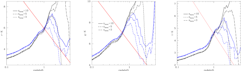
Figure 2.— Color-redshift diagrams for two PEGASE models at three formation redshifts. The upper tracks represent a solar metallicity instantaneous burst model with no obscuration, while the lower tracks show a zero initial metallicity exponentially declining star formation with $\tau=0.5\,$Gyr and “spheroid” extinction assumed. The diagonal lines represent $5\,\sigma$ limits in SDSS $g$, $r$, and $i$ bands. Objects above the diagonal line will not be detected in the individual SDSS band.

Figure 2 shows the $r-K$, $g-K$, and $i-K$ color-redshift diagrams for two sets of galaxy models generated with the spectral synthesis code PEGASE (Fioc & Rocca-Volmerange, 1997). The upper curves are color tracks for an instantaneous burst model at solar metallicity and assuming no extinction for formation redshifts of $z_{\rm form}=$ 10, 5, and 3, while the lower curves are for zero initial metallicity with an exponentially declining star-formation model with an $e$-folding time of $\tau=0.5\,$Gyr and PEGASE “spheroid” type obscuration at these same formation redshifts. We choose solar metallicity for the instantaneous burst model to match the $r-K$ color of an elliptical galaxy at low redshift, as the PEGASE models do not update the metallicity in an instantaneous burst. Metallicity does evolve in the models of ongoing star formation, hence the assumption of zero initial metallicity for the $\tau=0.5\,$Gyr $e$-folding star formation model. Although the spheroidal obscuration makes the ongoing star-formation model slightly redder than a typical elliptical galaxy at low redshift, we include it to approximate the effects of dust during the starburst (i.e. PEGASE does not allow for the destruction of dust). We would expect this model to be accurate at high redshift, but too red at low redshift. Since the low redshift models are excluded in both cases, this is not a concern. Shown for reference on each of the color redshift plots is the line representing the color of a point source at the $5\,\sigma$ limiting magnitude (AB) of the SDSS filter ($g_{\rm lim}=23.3$, $r_{\rm lim}=23.1$, $i_{\rm lim}=22.3$) with the $K$-band magnitude assumed from a linear fit to the $K-z$ diagram, given by: $K=4.62\,\log(z)+17.2$, derived from a fit to the galaxies in Van Bruegel et al. (1998). Sources below the line on the diagram would be detected in each SDSS band, while sources above would not. Note that there will be some scatter in the cutoff due to the scatter in the $K-z$ Hubble diagram. The exact nature of the objects passing the magnitude cut will depend on the color dependence of the scatter in th $K-z$ relation. Combining the information in the $K-z$ diagram and Figure 2 we see that all of the optically bright galaxies are either at low redshift, or galaxies very near their initial formation redshift. We can now use the optical properties of the radio galaxies to eliminate the low redshift component of the distribution.

Figure 3.— Monte-Carlo realization of the $dN/dz$ distribution of Figure 1. The shaded histogram represents objects that pass our optical color cuts, assuming that all galaxies have a formation redshift $z_{\rm form}=5.0$.

Figure 3 shows a Monte-Carlo realization of the $dN/dz$ distribution in Figure 1. The shaded histogram represents the galaxies that pass our selection criteria, assuming that all galaxies have the colors of the solar metallicity instantaneous burst with $z_{\rm form}=5$. These histograms show that using optical properties is an effective way of screening out the low redshift component of the radio galaxy population. The PEGASE models predict that the radio galaxies get much bluer and brighter in the optical near their formation epoch due to the initial burst of star formation in the models. As the histogram in Figure 3 shows, some fraction of these galaxies will be excluded from optically selected samples near their formation epoch as they become bright and blue enough to be detected in most optical surveys. These model colors are especially sensitive to the assumptions made for the star formation (e.g. obscuration, $e$-folding time), and it is difficult to infer how accurate these color tracks will be near the initial starburst. We also note that there is evidence for moderate obscuration in some high redshift galaxies (e.g., Dey, Spinrad, & Dickinson, 1995; Ouchi et al., 2004; Villar-Martin et al., 2005; Chary et al., 2005). Nevertheless, our models show that we may be somewhat biased against selecting unobscured galaxies with ongoing star formation near their formation epoch. Lowering the optical magnitude cutoff would allow these galaxies to enter our sample, although at the expense of the low redshift cutoff. Since we are primarily interested in galaxies with evolved stellar populations even at high redshift, as well as maintaining the efficiency of our search, we retain the optical selection to favor the low redshift cutoff at this minor expense of completeness.

2.1. Selection using SDSS and FIRST

We begin with the 2003 April 11 version of the FIRST catalog and select all sources with integrated flux $S_{\rm 1.4GHz}>100\,$mJy. The primary motivation for this cut is to define a manageable sample size. Flux limits as low as $\sim$10 mJy are reasonable for selecting high-redshift radio galaxies, and lower flux density limits will be explored in subsequent work. The $S_{\rm 1.4GHz}>100\,$mJy objects are positionally cross matched with photometric data from SDSS Data Release 2 (DR2), which covers more than 3300 square degrees. Objects with candidate identifications in any of the $u$, $g$, $r$, $i$ or $z$ bands within a conservative radius of $8^{\prime\prime}$ are excluded. Radio sources with no cataloged SDSS counterpart are visually inspected to further exclude possible low signal-to-noise optical counterparts, as well as identifying and excluding extended or multiple-lobe radio sources with an obvious optical counterpart located some distance from the cataloged radio position (an optical source lying between independently cataloged radio lobes, for example). Note that we are not restricted to unresolved radio sources: Our selection criteria allow for extended and multicomponent radio sources to be included as well. To further eliminate likely low redshift sources, we optimally combine (Szalay et al., 1999) the $g$, $r$, and $i$ SDSS images (the three most sensitive of the five SDSS filters) and eliminate any radio source with a candidate counterpart in the combined image.

The $5\,\sigma$ point source limiting AB magnitudes for SDSS are $u=22.3$, $g=23.3$, $r=23.1$, $i=22.3$, $z=20.8$, (Ivezic et al., 2000). The coadded $g$, $r$, and $i$ SDSS images allow us to extend the low redshift range being excluded by, in essence, improving our magnitude threshold by $\approx 1.0\,$magnitude. This can be roughly thought of as providing an effective $2\,\sigma$ $r$-band magnitude limit of $r\approx 24.1$, although the specific limiting value is dependent on the details of individual target galaxy SEDs. Coadded images are processed with SExtractor version 2.3.2 (Bertin & Arnouts, 1996), and any objects with a detection greater than $2\,\sigma$ above the background are excluded from the sample. Remaining target candidates are again visually inspected to eliminate new (faint) optical identifications of extended or multi-lobe radio sources. This visual inspection introduces some subjectivity into the target selection criteria, but it is necessary in order to eliminate obvious SDSS counterparts to double lobed radio sources, and sources that are extended in the FIRST catalog. Candidate targets with nearby bright stars or other nearby bright confusing sources are also excluded from the final target list. These targets are then checked against the NASA Extragalactic Database (NED) to screen out objects that had previously been observed. Only two objects, 4C $-$00.62 (Rottgering et al., 1997) and 3C 257, (Hewitt & Burbridge, 1991; Van Bruegel et al., 1998) were previously identified with confirmed redshifts of $z=2.53$ and $z=2.474$ respectively. The high redshift of these two radio galaxies support the effectiveness of our selection criteria. A final cut of ${\rm RA}>12\,$hr is made to eliminate targets not visible during our Spring observing runs. This process yields a total of 172 target objects. With 2085 $S_{\rm 1.4GHz}>100\,$mJy radio sources in this area of DR2, less than one in ten meet our selection criteria, giving us an order of magnitude improvement in efficiency of finding high redshift radio galaxies over blind spectroscopic targetting of all radio galaxies.

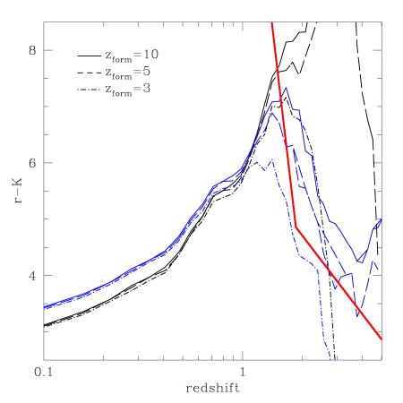
Figure 4.— Optical color cuts compared to model $r-K$ color as a function of redshift. Objects above and to the right of the thick line pass the selection.

Figure 4 shows a simulation of our multicolor optical selection in terms of $r-K$ color as a function of redshift for the same two sets of PEGASE spectral synthesis models used in Figure 2. The thick line shows the approximate effect of our optical selection criteria based on the $gri$ coaddition. Using the model $dN/dz$ of Dunlop and Peacock for radio sources brighter than $100\,$mJy with assumed pure luminosity evolution, we expect to exclude all sources with $z\,<\,1.7$ and an average redshift for the sample of $z\,\sim\,2.5$.

2.2. Selection on previous surveys

As a test of our selection criteria, we apply our selection to subsets of the galaxies in a blind radio survey (Best et al., 1999) and the ultra-steep spectrum (USS) sample of de Breuck et al. (2001). Of the 178 radio sources with spectroscopic redshifts in Best et al. (1999), only 20 fall within SDSS Data Release 3 (DR3). These sources have redshifts ranging from $z=0.004$ to $z=2.474$, a mean redshift of $z=0.78$, and a median of $z=0.66$. Applying our selection criteria leaves only two targets at redshifts of $z=1.339$ and $z=2.474$, the only galaxy with $z>1.5$ in the sample. Only 9 of the 62 USS sources of de Breuck et al. (2001) are within SDSS DR3, eight of which have firm redshifts. The mean and median redshift of this sample are 2.5 and 2.14 respectively. Applying our selection criteria eliminates the two $z<1$ galaxies from the sample, as well as one unusually optically bright galaxy with $z=2.48$, where Ly$\alpha$ falls in the $g$ band, and de Breuck et al. (2001) note that it has relatively strong continuum emission. The five remaining galaxies have a mean and median of $z=2.58$. As these two datasets show, our selection criteria is very effective at eliminating the low redshift foreground from both blind and USS samples. The exclusion of one $z>2$ galaxy illustrates the fact that our selection may eliminate some galaxies with strong observed frame optical emission, and we will explore the extent of this bias in a future paper.

3. The Observations

We aquired $K$-band images for 96 of the 172 unique candidates on the KPNO 4-meter Mayall telescope over two sets of four nights: 2003 April 20-23 and 2004 May 31 to 2004 June 3, using the Florida Multi-object Imaging Near-IR grism Observational Spectrometer (FLAMINGOS) instrument. The detector is a 2048x2048 HgCdTe wide-field IR imager and multi-slit spectrometer with a pixel size of $0.3165^{\prime\prime}$, which gives a $10.8^{\prime}\,\times\,10.8^{\prime}$ FOV on the 4 meter telescope. Conditions were highly variable during the 2003 run, with a night and a half lost due a combination of high wind and moisture (first night seeing $1.0^{\prime\prime}$ to $1.5^{\prime\prime}$, subsequent nights $1.0^{\prime\prime}$ to $2.3^{\prime\prime}$ due to combination of cloud, wind, and moisture). The 2004 run was photometric on all four nights with seeing varying from $0.7^{\prime\prime}$ to $1.2^{\prime\prime}$. Exposures were 20 seconds each in the 2003 run and 15 seconds each in 2004 to account for brighter sky levels. We observed in a fixed five point dither pattern with a separation of 30 arcseconds. Targets were observed for 15 minutes unless otherwise noted. The $5\,\sigma$ limiting magnitude in individual images spans $K\sim 19.0$. Three objects among those not detected after fifteen minutes were observed a second time. Objects J1411+0124, J1350+0352, and J2242-0808 have total integration times of 40, 61, and 29 minutes, respectively. J1123+0530 is the well known $z=2.474$ radio galaxy 3C 257 (Hewitt & Burbridge, 1991; Van Bruegel et al., 1998), one of the most luminous radio galaxies known. As it passed our selection criteria, it was observed in order to provide a consistency check with previous radio galaxy searches.

3.1. Reduction and Astrometry

We processed the data using standard NOAO IRAF routines. A set of dark frames were taken and subtracted from each image. A set of 6-10 adjacent (in time) images were combined to create a sky flat for subtraction (i.e. “running sky flats”). The images were approximately aligned based on the dither offsets, then the IRAF tasks mscgetcat and msccmatch were used to accurately register the images for coaddition. The IRAF task msccmatch uses a catalog of USNO-A2 (Monet et al., 1998) stellar positions and magnitudes for image registration and transformation, which may include image shift, scale change, and axis rotation. The resulting astrometry displayed a systematic offset on most images of between $0.5^{\prime\prime}$ to $1.0^{\prime\prime}$, due to slight differences between the USNO-A2 and SDSS astrometry. We manually corrected for these systematic offsets when constructing catalogs of each field. Our final astrometry is accurate to subarcsecond precision, with the residual difference between the $K$-band and SDSS positions well fit by gaussian of width $0.25^{\prime\prime}$.

3.2. Photometry

Each FLAMINGOS field was processed with SExtractor version 2.3.2. Quoted $K$-band magnitudes are SExtractor MAG$\_$AUTO unless otherwise noted. Due to the large field of view of the FLAMINGOS instrument, a large number ($\sim$100) of bright sources detected in the 2 Micron All Sky Survey (2MASS) are present in each field. Sources were cross matched with point sources from the 2MASS catalog having $K_{s}<15.3$, the $5\,\sigma$ limiting magnitude for point sources. Saturated stars were excluded from the comparison. A linear least squares fit between the SExtractor and 2MASS objects was perfomed to determine the zero point offset between the two datasets. This solution was assumed to continue linearly beyond the $K_{s}=15.3$ limit. Although we observed in $K$-band, while 2MASS uses $K_{s}$, no significant color terms were evident (the magnitude comparison between SExtractor and 2MASS was linear with a slope of unity). For radio galaxies not detected in $K$-band at the $2\,\sigma$ level, we report the $2\,\sigma$ magnitude of a point source as a lower limit.

3.3. Star-Galaxy Separation and ERO definition

The final $K$-band catalog was positionally cross matched with the SDSS catalog using a webservice interface to OpenSkyQuery (http://www.openskyquery.net) in order to obtain $r-K$ colors. A simple nearest neighbor criterion was used, and objects with no SDSS counterpart within a three arcsecond radius were assigned a $5\,\sigma$ limiting magnitude of $r=23.1$.

Star-Galaxy separation was done in two steps: For objects detected in SDSS with $r\leq 21.0$ we used the SDSS star-galaxy classification (probPSF, which is described in Scranton et al., 2002). For fainter $r$-band objects the separation was done by examining the difference between the $K$-band MAG$\_$AUTO magnitude (from SExtractor) and a fixed $3.5^{\prime\prime}$ aperture magnitude returned by SExtractor as a function of MAG$\_$AUTO to separate pointlike objects from extended galaxies.

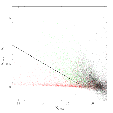
Figure 5.— $K_{\rm APER(3.5^{\prime\prime})}-K_{\rm AUTO}$ as a function of $K_{\rm AUTO}$. Red and green points are $r<21.0$ objects classified by SDSS as stars and galaxies respectively. Black points above and to the right of the black line are considered galaxies.

Figure 5 shows the resulting star-galaxy separation. This separation was chosen to be in rough agreement with the star-galaxy classification from SDSS where reliable classification was available. The slope of the resultant number counts for both stars and galaxies are in good agreement with those of Daddi et al. (2000). Reliable separation was possible to $K=17.0$, and objects fainter than this are considered to be galaxies.

The exact definition of EROs in the literature is not standardized. Some authors use total magnitudes (Wold et al., 2003; Cimatti et al., 2002a), some isophotal/aperture corrected (Daddi et al., 2000), some use matched aperture magnitudes in the $R$- and $K$-bands(e.g. Elston, Gonzalez et al., 2006), among others. There is the additional variation in the use of specific $R$ and $K$ (and $K_{s}$) filters used to select EROs, making comparison between ERO samples problematic. We chose our ERO definition by comparing to publicly available data in the Boötes field of the FLAMINGOS Extragalactic (FLAMEX) Survey (Elston, Gonzalez et al., 2006), which lies in the NOAO Deep Wide Field Survey (NDWFS) (Jannuzi & Dey, 1999), as well as SDSS. The Boötes field of the FLAMEX survey covers approximately 4.7 square degrees in both $J$- and $K_{s}$-bands. The FLAMEX survey was conducted with the FLAMINGOS instrument, and the its location within SDSS allows for a direct comparison with our data, although they use the $K_{s}$ filter where we use $K$. The FLAMEX survey defines EROs based on $6^{\prime\prime}$ matched aperture magnitudes in NDWFS $R$ and FLAMEX $K_{s}$ bands. Unfortunately, the SDSS catalog does not include aperture magnitudes, so we use SDSS model magnitudes in conjunction with $4^{\prime\prime}$ aperture magnitudes in $K$-band to define our $r-K$ color, as this aperture appears to best mimic the FLAMEX results. Cross-matching the FLAMEX, SDSS, and NDWFS data in a subset of the Boötes field, we found that an ERO definition of $r-K_{\rm APER(4^{\prime\prime})}\,\geq\,5.50$ approximated the $R-K_{S}\,\geq\,5.0$ definition of Elston, Gonzalez et al. (2006).

4. Results

4.1. The Radio Galaxies

The results of our $K$-band observations are shown in Tables 1 and 2. Table 1 lists objects detected, while Table 2 lists non-detections in the infrared. The column entries are:

1. Object Name: Name of source in IAU J2000 format. Objects with double lobe and multiple radio morphologies have the infrared object reported first and the individual radio components named a, b, c as necessary.

2. Date: Date observed.

3. Radio RA and DEC: Position of radio detection from the FIRST catalog (J2000)

4. $K$-band RA and DEC: Position of the infrared detected object (J2000)

5. Extended: Y if object shows visible extension in the FIRST image or if the object is a double or multiple lobe radio source. N if object is unresolved in the radio image.

6. $f_{\rm peak}$: Peak $1.4\,$GHz flux density from FIRST catalog (mJy)

7. $f_{\rm int}$: Interated $1.4\,$GHz flux density from FIRST catalog (mJy)

8. $K$: apparent magnitude and error for infrared object. Magnitudes are in the 2MASS system, which is slightly offset from the CIT system, given by: $K_{s}(\rm 2MASS)=K(\rm CIT)+0.0000\,\times\,(J-K)_{\rm CIT}-0.024\pm 0.003$ (Carpenter, 2001). For nondetections (Table 2) the $2\,\sigma$ detection limit is reported. Errors are those output by SExtractor.

9. Seeing: The full width half maximum seeing measured for the field, given in arcseconds.

10. $z_{K-z}$: estimated redshift based on a fit to the Hubble $K-z$ relation, given by $K=4.62\log(z)+17.2$. For nondetections (Table 2), the estimated redshift is given as a lower limit for the $2\,\sigma$ limiting magnitude.

We observe a total of 96 unique objects, detecting 70 of these at a $2\,\sigma$ level to a magnitude limit of $K\,\approx\,19.5$ in most cases. Three objects, J1102+0250, J1237+0135, and J1606+4751 show highly extended double radio lobes with complex morphologies. Subsequent visual inspection of the coadded $gri$ SDSS images for these objects reveals a probable optical counterpart that was missed in the original target selection. They thus do not meet our selection criteria, and we include them here merely for completeness. The total areal coverage of the $K$-band fields (exluding the field of J0742+3256, where a transient problem with the detector corrupted a portion of the field, but did not affect the radio galaxy target) is 8570 square arcminutes (2.38 square degrees). Of the 96 target objects, 27 are double lobed or multiple radio sources, having multiple components in the FIRST catalog. All but four of these multiple sources are identified in the NIR. Ten additional radio galaxies appear to be resolved in the radio postage images, and eight of these are identified with $K$-band counterparts.

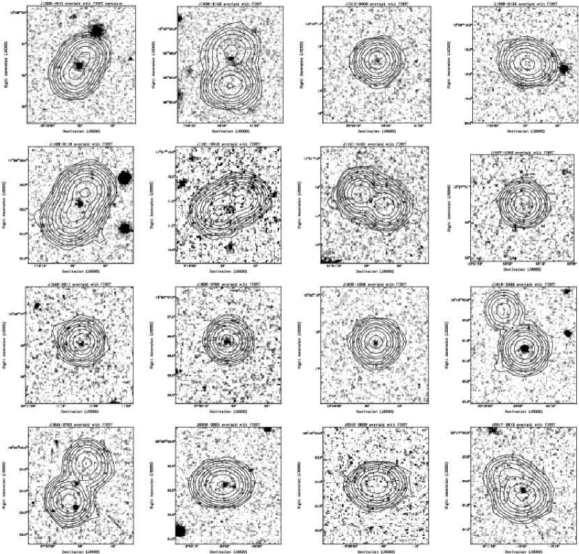
Figure 6.— A selection of $K$-band images. North is to the right and East is down. FIRST radio contours are overlaid with an outer contour at $5$mJy, and each subsequent contour indicating an increase by a factor of two.

Figure 6 shows images for a selection of our $K$-band detected objects. FIRST contours are overlaid with the outer contour at $5\,$mJy, and each subsequent contour indicating an increase by a factor of two. Postage stamp images for all galaxies can be found at http://lahmu.phyast.pitt.edu/dragons/.

Figure 7.— Distribution of $K$-band magnitudes for the observed objects. The filled histogram represents the $2\,\sigma$ limiting magnitudes of the non-detections. The solid vertical line represents the $K$-band magnitude for a galaxy at our expected lower redshift limit of $z=1.7$ and the shaded area represents the approximate scatter given the $K-z$ diagram at this redshift.

Figure 7 shows the distribution of $K$-band magnitudes for our observed objects. The solid histogram represents $2\,\sigma$ lower limits for our non-detections. The solid vertical line represents the magnitude of an object at our expected redshift cutoff of $z=1.7$, given our fit to the $K-z$ relation. The shaded region represents the approximate range of magnitudes for objects that follow the $K-z$ relation at this redshift.

Figure 8.— Estimated redshift distribution based on a linear fit to the $K-z$ Hubble diagram. The shaded histogram represents lower limit redshift estimates from the magnitude lower limits. The dashed histogram shows the distribution expected from convolving the Dunlop & Peacock (1990) $dN/dz$ with our selection criteria.

Figure 8 shows the estimated redshift distribution based on our linear fit to the $K-z$ Hubble diagram. Caution is advised in interpreting this histogram, because of the large intrinsic scatter in the $K-z$ diagram. The shaded portion of the histogram represents the lower limits on the estimated redshifts for the non-detected objects. The Monte-Carlo simulation of the Dunlop and Peacock $dN/dz$ convolved with our selection criteria from Figure 3 is shown for comparison. If we assign redshifts to the radio galaxies based on the linear fit to the $K-z$ diagram, the mean redshift for this sample is $z=2.5$ and the median redshift is $z=2.0$. Comparison with the expected redshift distribution in Figure 8 shows that we have 35 objects with $K<18.3$ that we expected to be excluded from our sample based on our model color tracks. While three of these objects are resolved in the radio images and subsequent closer examination revealed counterpart objects in SDSS, as indicated above, a full third of our sample are brighter in $K$ than expected. This can be partially attributed to the scatter in the $K-z$ relation if these galaxies are at the upper end of the redshift range given their $K$ magnitude. For example, the previously observed radio galaxy 3C 257 (J1123+0530) is known to be at $z=2.474$, while its $K=17.51$ magnitude corresponds to $z\sim 1.2$ on a linear fit to the $K-z$ diagram, indicative of the large intrinsic scatter in the $K-z$ relation. Van Bruegel et al. (1998) point out that $H\alpha$ falls into the $K$-band for 3C 257, which may explain its relative brightness in $K$. Similar line contamination may be responsible for some of the brighter than expected objects in our sample, but even this does not fully explain the brightest and reddest of our objects. Thirteen objects with $K<17.5$ have anomalously red $g-K$,$r-K$, and $i-K$ colors that are not fit by even our extreme model templates. Galactic r-band extinction from the SDSS database for these objects are listed in Table 3, based on the dust maps of Schlegel, Finkbeiner, & Davis (1998). There is a modest amount of extinction for three objects: J0941+0127, J1548+0036, and J1604-0013, though not enough to fully explain their extreme color. Applying the extinction model of Calzetti et al. (2000) to the non-evolving elliptical template of Coleman, Wu, & Weedman (1980) and assuming a redshift of near unity given by the $K-z$ diagram, we require extinctions of $A_{V}>0.5-1.5$ in order to reach the lower limit $r-K$ colors of these infrared bright sources. Determining spectroscopic redshifts for these objects will be the best way to determine whether the anomalously red colors are due to obscuration at lower redshift, a more luminous galaxy at higher redshift, or some combination of the two. These objects could also be a separate class not covered by our galaxy models, e.g. high redshift radio loud quasars or low redshift type II quasars where the AGN is completely obscured.

4.2. Radio Spectral Index

Table 4 shows the radio spectral index ($\alpha$, given by $S_{\nu}\propto\nu^{-\alpha}$) computed from FIRST and the Texas $365\,$MHz survey (Douglas et al., 1996). Van Bruegel et al. (1998) used an ultra-steep spectrum (USS) cut of $\alpha^{1400}_{365}>0.8$ to select a sample of high redshift radio galaxy candidates. Of our 96 targets, 75 have observations at $365\,$MHz, and of these 24 have $\alpha\,<\,0.8$ and would not be selected

Figure 9.— Spectral slope as a function of $z_{K-z}$ for the 75 targets with $S_{365\,MHz}$ flux densities measured in the Texas survey. The horizontal line represents the USS cut of Van Bruegel et al. (1998)

by the Van Bruegel et al. (1998) criteria. Figure 9 shows the spectral

Figure 10.— Histogram of redshifts inferred from the $K-z$ diagram divided into $\alpha\,<\,0.8$(shaded) and ultra-steep $\alpha\,>\,0.8$ emphasising the presence at high redshift ($z_{K-z}>2$) of flatter spectrum sources.

index of our targets as a function of $z_{K-z}$. Figure 10 shows a histogram of the redshifts inferred from the $K-z$ diagram for two spectral index ranges, flatter and steeper than $\alpha=0.8$. The median redshift of the $\alpha\,<\,0.8$ sample is $z_{K-z}=2.0$ and the mean is $z_{K-z}=2.13$, compared to a median of $z_{K-z}=2.0$ and mean $z_{K-z}=2.17$ for the total sample, and median $z_{K-z}=2.0$ and mean $z_{K-z}=2.30$ for the $\alpha\,>\,0.8$ sample. This suggests that flatter spectral slope systems may contribute a non-negligible fraction of the HzRG population. The insensitivity of our method to spectral slope allows us to select candidates that would be missed by USS selection techniques. Applying an USS criteria to our dataset would eliminate a full third of the targets.

Figure 11.— $1.4\,$GHz radio luminosity as a function of $K-z$ redshift. The lines represent $100\,$mJy (solid), $500\,$mJy (dashed), and $1\,$Jy (dot-dashed) flux density limits assuming a spectral slope $\alpha=0.4$. Squares mark objects with $\alpha^{1400}_{365}>0.8$, triangles indicate $\alpha^{1400}_{365}\leq 0.8$. The solid black circle marks the radio luminosity of 3C 257 with spectroscopic redshift $z=2.474$.

Figure 11 shows the $1.4\,GHz$ luminosities of the 75 galaxies given their $\alpha^{1400}_{365}$ and $K-z$ redshift. The three lines represent $100\,mJy$, $500\,mJy$, and $1\,Jy$ $1.4\,GHz$ flux limits, assuming $\alpha=0.4$.

Table 5 lists a subset of our candidates with additional radio observations at $4.85\,GHz$ (From Gregory & Condon, 1991) and $151\,MHz$ (From the 6C survey, Hales et al., 1988, 1990). This table shows the frequency dependence of the two point spectral slope. Several of the sources show significant deviations from a power law over the frequency range in question, showing that the USS sample selection will differ depending on frequencies used, while our selection method is unaffected by objects with concave radio spectra.

4.3. Environment

If, as we assert, high redshift radio galaxies form in the most overdense regions of the early Universe, then hierarchical formation scenarios predict an enhanced number of (proto-)galaxies associated with this overdensity. Although the strong spatial clustering of EROs is often attributed to association with high redshift galaxy overdensities, it is only recently that direct evidence for this has been found (Georgakakis et al., 2005). We search for overdensities of both EROs and $K$-band selected galaxies in the vicinity of our radio galaxy candidates. We begin with a consideration of the source counts of both $K$-band objects, as well as EROs.

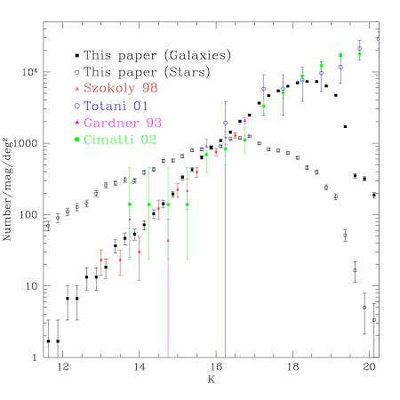
Figure 12.— Differential $K$-band galaxy number counts. For comparison the number counts of Gardner et al. (1993); Szokoly et al. (1998); Totani et al. (2001) and Cimatti et al. (2002b) are shown.

Figure 12 shows the $K$-band differential number counts for the galaxies and stars in our 95 fields. No completeness corrections have been applied. Plotted for comparison are counts from Gardner et al. (1993), Szokoly et al. (1998) ($K_{s}$), Totani et al. (2001), and Cimatti et al. (2002a) (from the $K20$ survey, also $K_{s}$). The raw counts are given in Table 6. As the Figure shows, we are in good agreement with previous infrared observations, and it appears that the radio galaxy target selection does not bias our $K$-band counts to the magnitude limits probed.

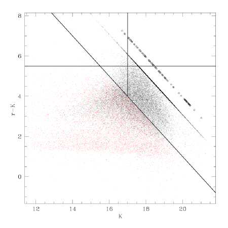
Figure 13.— $r-K$ as a function of $K$, showing star-galaxy separation and ERO definition. The diagonal upper limit in the measurements is due to the $5\,\sigma$ $r$-band limit from the SDSS assigned to non-detections, while the horizontal line marks the $r-K=5.50$ color used to define EROs. Red points are objects classified as stars, while black are galaxies. The diagonal line represents $r=21.0$, below which the SDSS star-galaxy separation is used. No star-galaxy separation is done for objects above this diagonal line and to the right of the vertical line at $K=17.0$. Open circles represent $2\,\sigma$ $r-K$ lower limits for the target radio galaxies in these fields.

Figure 13 shows the $r-K$ as a function of $K$ color-magnitude diagram after cross-matching our infrared catalog with the SDSS. We define an Extremely Red Object (ERO) as having $r-K\geq 5.50$ as indicated by the horizontal line on this Figure. Objects having no corresponding SDSS object within $3^{\prime\prime}$ are assigned a limiting magnitude of $r=23.1$. This yields

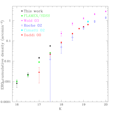
Figure 14.— Cumulative ERO surface density for our dataset and FLAMEX/SDSS. Shown for comparison are data from Daddi et al. (2000); Cimatti et al. (2002a); Roche et al. (2002) and Wold et al. (2003).

a total of 479 EROs, and Figure 14 shows the cumulative ERO surface density for this sample. Shown for comparison are the SDSS/FLAMEX ERO cumulative density for the $\approx$ 4.7 degrees² of the Boötes field. As can be seen, our ERO surface density for $K\,>\,17.0$ EROs is higher than the surface densities of both Daddi et al. (2000) and the FLAMEX/SDSS data, suggestive of an overdensity of EROs associated with our radio galaxy targets. Wold et al. (2003) observe EROs surrounding $z\sim 2$ radio loud quasars, and the Figure shows a higher ERO surface density than the “field” surveys of Roche et al. (2002), Daddi et al. (2000), and Cimatti et al. (2002a). Our data seem to show a continuation of the trend seen by Wold et al. (2003). Because of the $r=23.1$ limit from SDSS we are limited to studying $K\leq 17.60$ EROs. Due to the small areas covered by previous ERO studies, surface densities at this bright K magnitude are uncertain. $5.9\%$ (30 out of 509) of our EROs are classified as stars, smaller than the $\approx 9\%$ of Manucci et al. (2002) and Wold et al. (2003), which may be a concern. At these bright $K$-band magnitudes, robust star galaxy separation is increasingly important. We note, again, that our overall star and galaxy counts are in good agreement with Daddi et al. (2000) in the relevant magnitude range, leading us to believe that our star-galaxy separation is robust. Figure 12 shows that our $K$-band number counts are consistent with previous surveys, yet our ERO density is higher at $K>17.0$ than in the same surveys. This is because only a small percentage of the $K$-band selected galaxies are EROs, and the increase in this rare population is small compared to the overall galaxy counts. Thus, the EROs appear to trace an overdensity not readily apparent in the $K$-band data alone, as pointed out by Wold et al. (2003).

We now examine the clustering of EROs around our radio galaxies. We restrict our analysis to $K\,\leq\,17.50$ EROs in order to remain complete given the $r_{\rm lim}=23.1$ magnitude limit of our SDSS data. Because we expect the radio galaxy to be, by far, the most luminous galaxy in its local environment, we expect to see a possible overdensity around only the brightest of our targets. An overdensity of EROs with $K$-band magnitudes brighter than the radio galaxy would be a possible indication of a foreground structure. Field by field, the density of EROs is quite inhomogeneous, as expected. More than half of the fields have no bright EROs within $100^{\prime\prime}$ of the radio galaxy target, while seven fields have three or more EROs within this radius. The seven densest fields have radio galaxy targets with magnitudes evenly spaced in the range $K=17.4-20.6$, showing no trend of high ERO density with radio galaxy NIR brightness, contrary to

Figure 15.— Average surface density of $K<17.50$ EROs as a function of radial distance from the radio galaxy for 95 target fields. The four panels are subsamples selected by the $K$-band magnitude of the target radio galaxy. The horizontal line represents the “local field density” of the sample, defined as the average surface density of EROs between $120^{\prime\prime}$ and $180^{\prime\prime}$ from the radio source.

our expectations. Figure 15 shows the average distribution of EROs with $K\leq 17.50$ as a function of radial distance from the radio galaxy for 95 of our target fields. We do not include the radio galaxy itself, although some are EROs. The horizontal line is a measure of the “local field” density of EROs, defined as the density of EROs between $120^{\prime\prime}$ and $180^{\prime\prime}$ from the radio source. There is a modest overdensity of EROs within an arcminute of the radio targets, although the uncertainties are very large. Wold et al. (2003) perform a similar analysis and see no such evidence for clustering for EROs brighter than $K_{s}\,=\,19.5$ around their $z\,\sim\,2$ radio loud quasars. A deeper sample of EROs is necessary for a complete analysis of the radio galaxy environment. This could be established from our existing data through the addition of deep $R$-band imaging ($R\,\approx\,25$), and we are actively pursuing this goal. Deep $R$-band imaging would also allow for more rigorous star-galaxy separation to fainter magnitudes, to better determine the stellar contamination of our ERO population.

Figure 16.— Surface density of $K<19.0$ galaxies as a function of radial distance from the radio galaxy. The four panels are subsamples selected by the $K$-band magnitude of the target radio galaxy. The horizontal line in each panel represents the “local field density” of $K$-band selected galaxies, defined as the average surface density of galaxies between $120^{\prime\prime}$ and $180^{\prime\prime}$ from the radio source.

Figure 16 shows the distribution of $K\,<\,19.0$ galaxies around our targets. The four panels of Figure 16 represent the division of the sample by the apparent magnitude of the target radio galaxy. Given the $K-z$ Hubble diagram, this is a rough proxy for redshift. The horizontal line in each panel shows a measure of the ”local field” density of galaxies (defined as the density of objects between $120^{\prime\prime}$ and $180^{\prime\prime}$ from the radio source). No clustering is seen in any of the bins. This is not unexpected, as Hall & Green (1998) and Hall et al. (2001) do not see an excess around $z\approx 1.5$ radio loud quasars below $K=19$, but do see an excess of galaxies at $K=19-20.5$. Deeper $K$-band imaging is necessary to detect possible companion galaxies at the high redshifts of our radio galaxy targets. Such imaging will be conducted on future additions to our target sample (see § 5 for details).

5. Summary and Future Work

Using a novel radio-optical selection technique, we have obtained NIR imaging for 96 HzRG candidates. Based on redshift estimates from the $K-z$ Hubble diagram, our new selection technique appears to be effective at identifying HzRGs, as more than half of our targets have $K$-band photometry consistent with $z>2$. This technique is not sensitive to radio spectral slope, and avoids the frequency dependence of USS techniques for galaxies with non-power law radio spectra. Of the 75 target galaxies present in the Texas 365 MHz survey 24 have $\alpha^{\rm 1.4GHz}_{\rm 365MHz}<0.8$. These would be excluded by the USS criteria of Van Bruegel et al. (1998), and all but four of these 75 have $\alpha^{\rm 1.4GHz}_{\rm 365MHz}<1.3$, which would be excluded from more recent USS selections (e.g. de Breuck et al., 2001; Jarvis et al., 2001). Comparison with the previous surveys of Best et al. (1999) and de Breuck et al. (2001) shows that our technique selects nearly all of their high redshift targets, while also eliminating the low redshift sources. The $K$-band number counts are consistent with previous work, and the large non-contiguous area (2.38 square degrees) covered by the DRaGONS survey to date makes it an excellent resource for exploring galaxy properties through the combination of NIR and optical data.

We have uncovered a previously unseen class of radio sources with anomalously red colors ($r-K\,>\,6.5-7$), which may be evidence of significant obscuration at moderate redshifts. These galaxies represent more than ten percent of our observed sample, indicating that they may be a substantial percentage of the radio galaxy population. Being non-detections in SDSS (with $r\,>\,24.1$), current optical AGN selection techniques are insensitive to these sources. Radio loud QSOs comprise only $\sim\,5-10\%$ of overall QSOs; therefore, these objects could represent a significant contribution to radio loud AGNs that are not counted in current samples.

We have identified a sample of 479 EROs to a depth of $K=17.50$, one of the largest bright ERO samples to date, and have identified a modest overdensity of EROs around our HzRG candidates. We do not detect any similar overdensity when all the $K$-band selected galaxies to $K=19.0$ are considered.

Spectroscopic follow up of the radio galaxy candidates and the surrounding EROs is of the utmost importance, both for validation of our HzRG candidates, as well as determination of the relationship between the radio galaxies and the ERO overdensity. Firm redshifts will also allow us to accurately test the $z-\alpha$ relation for our non-USS selected sample. Near infrared spectroscopy of the anomalously red radio galaxies should pinpoint the cause of their extreme colors, as well as determine the amount of obscuration present at intermediate and high redshifts.

Deeper optical imaging is required in order to establish colors for the radio galaxies and explore their morphology in more detail. Deeper optical imaging will also allow us to select a deeper and more complete sample of EROs, allowing for a more detailed study of the radio galaxy environment and the nature of the ERO overdensity. A more quantitative study of ERO clustering will also be possible with deeper optical data (including a two-point angular correlation function analysis).

A future paper will also examine the effects of both our radio flux density cut, as well as our optical color cuts. In future observing runs we plan to target a small sample of lower flux density radio sources that meet our optical color cuts. We will supplement this sample with galaxies from the FLAMEX survey that meet our selection criteria. This dataset will allow us to examine any biases introduced by our radio selection. Several of the targets in our most recent round of observing lie in the SDSS Southern Survey, an area of SDSS that is more than four times more sensitive than the standard SDSS survey. This deeper imaging data will allow us to study the optical properties of those targets that are detected.

Table 1Detections

Object Name	date	radio RA	radio DEC	Extended?	K RA	K DEC	$f_{\rm peak}$(mJy)	$f_{\rm int}$(mJy)	K	seeing(′′)	$z_{K-z}\tablenotemark{b}$
J0742+3256	23 April 2003	07:42:13.61	+32:56:51.16	N	07:42:13.60	+32:56:51.20	130.51	144.60	17.72$\pm$0.08	1.0	1.3
J0831+5210	23 April 2003	$\cdots$	$\cdots$	Y	08:31:44.83	+52:10:34.95	$\cdots$	$\cdots$	18.93$\pm$0.17	1.1	2.4
a	$\cdots$	08:31:44.89	+52:10:41.28	$\cdots$	$\cdots$	$\cdots$	97.07	113.73	$\cdots$	$\cdots$	$\cdots$
b	$\cdots$	08:31:44.74	+52:10:28.72	$\cdots$	$\cdots$	$\cdots$	108.06	131.18	$\cdots$	$\cdots$	$\cdots$
J0941+0127	23 April 2003	09:41:48.75	+01:27:36.45	N	09:41:48.77	+01:27:35.89	117.82	120.56	17.17$\pm$0.08	2.2	1.0
J0958+0324	20 April 2003	$\cdots$	$\cdots$	Y	09:58:24.95	+03:24:13.56	$\cdots$	$\cdots$	17.46$\pm$0.09	1.5	1.1
a	$\cdots$	09:58:24.18	+03:24:20.84	$\cdots$	$\cdots$	$\cdots$	72.53	190.15	$\cdots$	$\cdots$	$\cdots$
b	$\cdots$	09:58:23.57	+03:24:24.98	$\cdots$	$\cdots$	$\cdots$	125.58	162.14	$\cdots$	$\cdots$	$\cdots$
c	$\cdots$	09:58:26.323	+03:24:01.51	$\cdots$	$\cdots$	$\cdots$	166.91	286.56	$\cdots$	$\cdots$	$\cdots$
J1102+0250	21 April 2003	$\cdots$	$\cdots$	Y	11:02:06.59	+02:50:45.45	$\cdots$	$\cdots$	16.70$\pm$0.06	2.1	0.8
a	$\cdots$	11:02:05.66	+02:50:58.19	$\cdots$	$\cdots$	$\cdots$	29.48	127.69	$\cdots$	$\cdots$	$\cdots$
b	$\cdots$	11:02:06.05	+02:50:48.86	$\cdots$	$\cdots$	$\cdots$	8.71	33.29	$\cdots$	$\cdots$	$\cdots$
J1123+0530	23 April 2003	$\cdots$	$\cdots$	Y	11:23:09.43	+05:30:18.60	$\cdots$	$\cdots$	17.51$\pm$0.11	1.7	1.2
a	$\cdots$	11:23:09.06	+05:30:20.58	$\cdots$	$\cdots$	$\cdots$	1514.62	1580.13	$\cdots$	$\cdots$	$\cdots$
b	$\cdots$	11:23:09.75	+05:30:13.83	$\cdots$	$\cdots$	$\cdots$	150.31	163.07	$\cdots$	$\cdots$	$\cdots$
J1135+0548	21 April 2003	11:35:17.81	+05:48:54.13	N	11:35:17.84	+05:48:54.06	190.84	212.63	18.77$\pm$0.15	2.1	2.2
J1155+0305	20 April 2003	$\cdots$	$\cdots$	Y	11:55:12.48	+03:05:18.93			17.36$\pm$0.06	1.1	1.1
a	$\cdots$	11:55:11.94	+03:05:25.69	$\cdots$	$\cdots$	$\cdots$	40.01	57.21	$\cdots$	$\cdots$	$\cdots$
b	$\cdots$	11:55:12.80	+03:05:14.61	$\cdots$	$\cdots$	$\cdots$	77.26	105.60	$\cdots$	$\cdots$	$\cdots$
J1208+0414	21 April 2003	$\cdots$	$\cdots$	Y	12:08:11.90	+04:14:59.37	$\cdots$	$\cdots$	18.15$\pm$0.14	1.7	1.6
a	$\cdots$	12:08:11.69	+04:15:04.87	$\cdots$	$\cdots$	$\cdots$	204.08	299.15	$\cdots$	$\cdots$	$\cdots$
b	$\cdots$	12:08:12.24	+04:14:55.55	$\cdots$	$\cdots$	$\cdots$	264.65	341.17	$\cdots$	$\cdots$	$\cdots$
J1208+4943	01 June 2004	$\cdots$	$\cdots$	Y	12:08:24.73	+49:43:29.72	$\cdots$	$\cdots$	17.03$\pm$0.04	0.8	0.9
a	$\cdots$	12:08:24.04	+49:43:31.74	$\cdots$	$\cdots$	$\cdots$	78.12	87.72	$\cdots$	$\cdots$	$\cdots$
b	$\cdots$	12:08:24.94	+49:43:28.61	$\cdots$	$\cdots$	$\cdots$	88.83	111.26	$\cdots$	$\cdots$	$\cdots$
J1236+0150	02 June 2004	12:36:00.15	+01:50:52.59	Y	12:35:59.60	+01:50:52.79	144.70	154.53	17.25$\pm$0.07	0.9	1.0
J1237+0135	20 April 2003	$\cdots$	$\cdots$	Y	12:37:05.32	+01:35:53.27	$\cdots$	$\cdots$	17.96$\pm$0.07	0.9	1.5
a	$\cdots$	12:37:7.681	+01:35:58.08	$\cdots$	$\cdots$	$\cdots$	162.2	193.99	$\cdots$	$\cdots$	$\cdots$
b	$\cdots$	12:37:3.252	+01:35:53.98	$\cdots$	$\cdots$	$\cdots$	180.7	232.25	$\cdots$	$\cdots$	$\cdots$
J1250+6043	04 June 2004	12:50:24.47	+60:43:46.84	N	12:50:24.47	+60:43:46.59	288.67	304.05	17.81$\pm$0.09	1.1	1.4
J1259+0559	23 April 2003	$\cdots$	$\cdots$	Y	12:59:12.37	+05:59:03.10	$\cdots$	$\cdots$	18.36$\pm$0.14	1.9	1.8
a	$\cdots$	12:59:11.93	+05:59:29.05	$\cdots$	$\cdots$	$\cdots$	66.15	73.60	$\cdots$	$\cdots$	$\cdots$
b	$\cdots$	12:59:12.57	+05:58:52.43	$\cdots$	$\cdots$	$\cdots$	53.98	105.19	$\cdots$	$\cdots$	$\cdots$
J1308$-$0022	03 June 2004	$\cdots$	$\cdots$	Y	13:08:56.17	$-$00:22:36.65	$\cdots$	$\cdots$	19.05$\pm$0.15	1.1	2.5
a	$\cdots$	13:08:56.36	$-$00:22:33.12	$\cdots$	$\cdots$	$\cdots$	90.77	98.14	$\cdots$	$\cdots$	$\cdots$
b	$\cdots$	13:08:55.87	$-$00:22:42.98	$\cdots$	$\cdots$	$\cdots$	134.01	143.03	$\cdots$	$\cdots$	$\cdots$
J1312+0009	20 April 2003	13:12:32.83	+00:09:13.40	N	13:12:32.79	+00:09:13.17	109.42	112.61	19.03$\pm$0.17	1.1	2.5
J1313+6250	02 June 2004	13:13:15.63	+62:50:47.29	N	13:13:15.63	+62:50:47.36	128.32	132.18	18.43$\pm$0.10	1.1	1.8
J1315+0533	04 June 2004	13:15:17.92	+05:33:14.07	N	13:15:18.00	+05:33:09.93	140.25	146.96	18.72$\pm$0.13	1.0	2.1
J1332+0101	23 April 2003	$\cdots$	$\cdots$	Y	13:32:16.55	+01:01:48.26	$\cdots$	$\cdots$	17.05$\pm$0.08	2.0	0.9
a	$\cdots$	13:32:16.78	+01:01:50.83	$\cdots$	$\cdots$	$\cdots$	152.34	228.66	$\cdots$	$\cdots$	$\cdots$
b	$\cdots$	13:32:15.94	+01:01:40.81	$\cdots$	$\cdots$	$\cdots$	118.60	184.03	$\cdots$	$\cdots$	$\cdots$
J1336+0207	03 June 2004	13:36:34.43	+02:07:37.13	Y	13:36:34.33	+02:07:42.21	113.55	127.76	19.20$\pm$0.18	0.9	2.7
J1400+0053	21 April 2003	14:00:4.59	+00:53:19.0	N	14:00:04.64	+00:53:18.90	112.87	130.80	17.23$\pm$0.08	1.4	1.0
J1402+0342	23 April 2003	14:02:24.86	+03:42:27.10	N	14:02:24.89	+03:42:26.73	501.26	540.42	17.65$\pm$0.10	1.7	1.2
J1403+6048	04 June 2004	14:03:59.55	+60:48:07.85	N	14:03:59.62	+60:48:07.69	526.50	794.62	17.55$\pm$0.07	0.8	1.2
J1408+0116	02 June 2004	$\cdots$	$\cdots$	Y	14:08:33.38	+01:16:22.24	$\cdots$	$\cdots$	17.08$\pm$0.05	0.8	0.9
a	$\cdots$	14:08:33.13	+01:16:23.99	$\cdots$	$\cdots$	$\cdots$	290.25	320.12	$\cdots$	$\cdots$	$\cdots$
b	$\cdots$	14:08:33.58	+01:16:20.85	$\cdots$	$\cdots$	$\cdots$	199.15	292.63	$\cdots$	$\cdots$	$\cdots$
J1411+0124	20-21 April 2003	$\cdots$	$\cdots$	Y	14:11:08.29	+01:24:40.56	$\cdots$	$\cdots$	19.93$\pm$0.18	1.3	3.9
a	$\cdots$	14:11:08.32	+01:24:45.48	$\cdots$	$\cdots$	$\cdots$	116.43	122.32	$\cdots$	$\cdots$	$\cdots$
b	$\cdots$	14:11:08.21	+01:24:33.78	$\cdots$	$\cdots$	$\cdots$	60.89	64.17	$\cdots$	$\cdots$	$\cdots$
J1423+0139	23 April 2003	14:23:03.45	+01:39:58.23	N	14:23:03.47	+01:39:58.46	202.21	211.64	17.37$\pm$0.09	2.0	1.1
J1438+0150	20 April 2003	14:38:17.15	+01:50:31.05	N	14:38:17.20	+01:50:31.27	83.24	118.52	17.94$\pm$0.17	1.0	1.4
J1438+6149	03 June 2004	14:38:41.83	+61:49:33.79	N	14:38:41.87	+61:49:33.67	114.73	121.27	18.70$\pm$0.14	0.8	2.1
J1451+5404	01 June 2004	$\cdots$	$\cdots$	Y	14:51:43.43	+54:04:22.02	$\cdots$	$\cdots$	19.37$\pm$0.20	0.9	2.9
a	$\cdots$	14:51:43.66	+54:04:25.67	$\cdots$	$\cdots$	$\cdots$	265.89	274.33	$\cdots$	$\cdots$	$\cdots$
b	$\cdots$	14:51:43.23	+54:04:25.67	$\cdots$	$\cdots$	$\cdots$	271.59	280.30	$\cdots$	$\cdots$	$\cdots$
J1452+0032	21 April 2003	$\cdots$	$\cdots$	Y	14:52:00.78	+00:32:45.54	$\cdots$	$\cdots$	17.92$\pm$0.09	1.3	1.4
a	$\cdots$	14:52:01.46	+00:33:01.29	$\cdots$	$\cdots$	$\cdots$	112.59	143.03	$\cdots$	$\cdots$	$\cdots$
b	$\cdots$	14:51:59.91	+00:32:41.68	$\cdots$	$\cdots$	$\cdots$	471.04	496.02	$\cdots$	$\cdots$	$\cdots$
J1510+5244	03 June 2004	15:10:20.20	+52:44:30.20	N	15:10:20.16	+52:44:30.68	500.50	505.76	18.41$\pm$0.18	0.8	1.8
J1515+5744	20 April 2003	15:15:29.30	+57:44:57.32	Y	15:15:29.33	+57:44:56.25	78.56	144.16	19.14$\pm$0.18	1.0	2.6
J1523$-$0018	01 June 2004	15:23:16.19	$-$00:18:55.40	Y	15:23:16.23	$-$00:18:55.08	216.42	231.44	18.75$\pm$0.10	0.9	2.2
J1526+0408	23 April 2003	$\cdots$	$\cdots$	Y	15:26:37.15	+04:08:14.22	$\cdots$	$\cdots$	17.87$\pm$0.11	2.0	1.4
a	$\cdots$	15:26:38.90	+04:08:02.96	$\cdots$	$\cdots$	$\cdots$	18.14	53.66	$\cdots$	$\cdots$	$\cdots$
b	$\cdots$	15:26:36.59	+04:08:19.72	$\cdots$	$\cdots$	$\cdots$	43.55	102.76	$\cdots$	$\cdots$	$\cdots$
J1532+4432	04 June 2004	$\cdots$	$\cdots$	Y	15:32:50.13	+44:32:15.24	$\cdots$	$\cdots$	17.16$\pm$0.08	0.9	1.0
a	$\cdots$	15:32:50.85	+44:32:16.86	$\cdots$	$\cdots$	$\cdots$	92.53	117.98	$\cdots$	$\cdots$	$\cdots$
b	$\cdots$	15:32:49.66	+44:32:14.50	$\cdots$	$\cdots$	$\cdots$	86.96	131.67	$\cdots$	$\cdots$	$\cdots$
J1541+5259	23 April 2003	$\cdots$	$\cdots$	Y	15:41:18.87	+52:59:55.38	$\cdots$	$\cdots$	17.24$\pm$0.08	2.3	1.0
a	$\cdots$	15:41:18.75	+52:59:52.35	$\cdots$	$\cdots$	$\cdots$	100.27	115.12	$\cdots$	$\cdots$	$\cdots$
b	$\cdots$	15:41:18.81	+53:00:00.38	$\cdots$	$\cdots$	$\cdots$	67.11	77.90	$\cdots$	$\cdots$	$\cdots$
J1543+5711	03 June 2004	15:43:30.33	+57:11:32.40	Y	15:43:30.12	+57:11:32.37	55.88	103.39	18.24$\pm$0.08	0.9	1.7
J1547+4839	04 June 2004	15:47:42.06	+48:39:12.20	N	15:47:42.34	+48:39:09.33	186.86	214.75	19.49$\pm$0.18	0.9	3.1
J1548+0036	21 April 2003	15:48:16.21	+00:36:13.56	Y	15:48:16.22	+00:36:13.27	123.08	126.05	16.83$\pm$ 0.04	1.7	0.8
J1548$-$0033	20 April 2003	$\cdots$	$\cdots$	Y	15:48:21.75	$-$00:34:00.80	$\cdots$	$\cdots$	19.06$\pm$0.14	0.9	2.5
a	$\cdots$	15:48:21.45	$-$00:33:59.28	$\cdots$	$\cdots$	$\cdots$	155.03	231.62	$\cdots$	$\cdots$	$\cdots$
b	$\cdots$	15:48:22.14	$-$00:34:00.64	$\cdots$	$\cdots$	$\cdots$	157.66	201.46	$\cdots$	$\cdots$	$\cdots$
J1549+4719	04 June 2004	15:49:53.47	+47:19:48.56	N	15:49:53.53	+47:19:48.25	104.66	106.33	18.20$\pm$0.11	0.9	1.6
J1554+4729	04 June 2004	15:54:25.63	+47:29:00.97	N	15:54:25.67	+47:29:00.56	137.54	149.73	18.70$\pm$0.09	0.9	2.1
J1559+5011	03 June 2004	15:59:47.89	+50:11:16.41	N	15:59:47.96	+50:11:16.44	127.0	130.28	18.38$\pm$0.11	0.8	1.8
J1604$-$0013	02 June 2004	16:04:12.71	$-$00:13:41.89	N	16:04:12.62	$-$00:13:41.28	117.91	128.28	17.13$\pm$0.05	0.9	1.0
J1604+4746	22 April 2003	16:04:27.85	+47:46:35.02	N	16:04:27.92	+47:46:34.48	351.96	366.10	18.70$\pm$0.13	1.3	2.1
J1606+4751	04 June 2004	16:06:1.29	+47:51:52.17	Y	16:06:01.40	+47:51:46.30	3.07	12.31	17.47$\pm$0.07	0.9	1.1
a	$\cdots$	16:06:1.82	+47:52:01.68	$\cdots$	$\cdots$	$\cdots$	36.38	61.54	$\cdots$	$\cdots$	$\cdots$
b	$\cdots$	16:06:2.49	+47:51:21.20	$\cdots$	$\cdots$	$\cdots$	81.73	109.02	$\cdots$	$\cdots$	$\cdots$
J1609+3700	03 June 2004	16:09:28.11	+37:00:18.12	N	16:09:28.13	+37:00:18.0	96.52	102.52	17.80$\pm$0.08	0.8	1.3
J1617+4848	23 April 2003	16:17:25.42	+48:48:28.69	N	16:17:25.47	+48:48:28.38	236.95	244.32	18.00$\pm$0.11	1.9	1.5
J1629+4937	20 April 2003	16:29:21.38	+49:37:54.86	N	16:29:21.31	+49:37:54.27	183.38	197.05	19.50$\pm$0.19	1.0	3.1
J1632+4056	01 June 2004	16:32:16.27	+40:56:32.71	N	16:32:16.29	+40:56:32.63	200.82	203.15	18.89$\pm$0.13	0.8	2.3
J1634+4155	03 June 2004	16:34:43.60	+41:55:03.40	N	16:34:43.57	+41:55:03.09	216.39	263.47	18.30$\pm$0.11	0.8	1.7
J1636+4808	21 April 2003	$\cdots$	$\cdots$	Y	16:36:15.70	+48:08:48.32	$\cdots$	$\cdots$	19.10$\pm$0.17	1.2	2.6
a	$\cdots$	16:36:16.04	+48:08:50.11	$\cdots$	$\cdots$	$\cdots$	87.46	97.73	$\cdots$	$\cdots$	$\cdots$
b	$\cdots$	16:36:15.16	+48:08:45.59	$\cdots$	$\cdots$	$\cdots$	147.42	165.66	$\cdots$	$\cdots$	$\cdots$
J1637+3223	03 June 2004	16:37:34.53	+32:23:05.84	N	16:37:34.53	+32:23:06.21	136.29	147.47	18.80$\pm$0.15	0.8	2.2
J1643+4518	03 June 2004	16:43:22.62	+45:18:06.68	N	16:43:22.79	+45:18:01.68	108.30	110.39	18.30$\pm$0.11	0.8	1.7
J1645+4152	03 June 2004	16:45:00.73	+41:52:14.20	N	16:45:00.80	+41:52:14.30	112.56	115.96	18.42$\pm$0.09	0.8	1.8
J1648+4233	23 April 2003	16:48:31.51	+42:33:22.42	Y	16:48:31.52	+42:33:21.82	167.44	169.30	19.00$\pm$0.17	2.1	2.5
J1649+3350	02 June 2004	16:49:24.21	+33:50:02.04	N	16:49:24.19	+33:50:02.17	162.25	163.91	16.86$\pm$0.03	0.9	0.8
J1654+4125	02 June 2004	16:54:43.87	+41:25:02.96	N	16:54:43.89	+41:25:03.00	225.60	228.56	18.15$\pm$0.10	0.9	1.6
J1655+2723	01 June 2004	$\cdots$	$\cdots$	Y	16:55:04.33	+27:23:28.91	$\cdots$	$\cdots$	18.52$\pm$0.09	0.8	1.9
a	$\cdots$	16:55:03.87	+27:23:32.00	$\cdots$	$\cdots$	$\cdots$	40.01	54.13	$\cdots$	$\cdots$	$\cdots$
b	$\cdots$	16:55:04.73	+23:23:26.47	$\cdots$	$\cdots$	$\cdots$	101.27	115.40	$\cdots$	$\cdots$	$\cdots$
J1656+2707	02 June 2004	16:56:16.29	+27:07:32.47	N	16:56:16.31	+27:07:33.05	160.33	164.76	18.88$\pm$0.15	0.9	2.3
J1707+2408	01 June 2004	17:07:44.58	+24:08:54.56	N	17:07:44.57	+24:08:54.41	144.83	169.15	17.96$\pm$0.09	0.8	1.5
J1715+3027	01 June 2004	17:15:48.29	+30:27:23.18	N	17:15:48.31	+30:27:23.18	378.27	385.34	18.54$\pm$0.09	0.8	2.0
J2059$-$0603	02 June 2004	20:59:32.88	$-$06:03:00.34	N	20:59:32.87	$-$06:02:59.59	155.63	161.72	18.32$\pm$0.10	0.9	1.7
J2107$-$0701	02 June 2004	21:07:45.46	$-$07:01:07.83	N	21:07:45.47	$-$07:01:06.54	523.60	550.60	18.37$\pm$0.09	0.9	1.8
J2223$-$0757	01 June 2004	22:23:26.52	$-$07:57:08.07	N	22:23:26.51	$-$07:57:06.94	104.79	108.34	17.70$\pm$0.08	0.9	1.3
J2247$-$0910	01 June 2004	22:47:23.79	$-$09:10:49.74	Y	22:47:23.69	$-$09:10:49.26	77.10	103.37	17.99$\pm$0.09	0.9	1.5
J2309$-$0834	03 June 2004	23:09:04.29	$-$08:34:57.19	N	23:09:4.29	$-$08:34:56.83	103.19	111.67	18.23$\pm$0.12	0.9	1.7
J2316$-$0846	03 June 2004	23:16:35.08	$-$08:46:17.72	N	23:16:35.07	$-$08:46:17.16	101.85	105.40	18.59$\pm$0.14	0.9	2.0
J2336$-$0838	04 June 2004	$\cdots$	$\cdots$	Y	23:36:18.35	$-$08:38:48.87	$\cdots$	$\cdots$	18.50$\pm$0.15	0.9	1.9
a	$\cdots$	23:36:18.11	$-$08:38:43.58	$\cdots$	$\cdots$	$\cdots$	124.78	134.50	$\cdots$	$\cdots$	$\cdots$
b	$\cdots$	23:36:18.65	$-$08:38:48.27	$\cdots$	$\cdots$	$\cdots$	104.16	110.32	$\cdots$	$\cdots$	$\cdots$
J2337$-$0852	04 June 2004	23:37:32.44	$-$08:52:39.49	N	23:37:32.46	$-$08:52:38.83	118.04	120.14	18.20$\pm$0.13	0.9	1.6

Table 2Non-Detections

Object Name	date	radio RA	radio DEC	Extended?	$f_{\rm peak}$(mJy)	$f_{\rm int}$(mJy)	K ($2\,\sigma$)	seeing(′′)	$z_{K-z}$
J1022+0357	23 April 2003	10:22:01.03	+03:57:37.56	N	194.31	200.86	$>$20.11	2.3	$>$3.2
J1028+0144	21 April 2003	10:28:02.79	+01:44:06.51	Y	56.82	114.81	$>$19.80	2.0	$>$2.7
J1044+0538	20 April 2003	10:44:19.88	+05:38:07.98	N	125.54	130.20	$>$20.32	1.2	$>$3.5
J1047+0216	23 April 2003	10:47:11.32	+02:16:28.21	N	122.32	125.81	$>$20.09	2.2	$>$3.1
J1144+0254	23 April 2003	11:44:34.26	+02:54:25.56	N	114.01	119.18	$>$20.13	2.1	$>$3.2
J1221+0248	23 April 2003	12:21:39.93	+02:48:28.01	N	139.93	142.87	$>$20.13	1.9	$>$3.2
J1234+0024	03 June 2004	12:34:30.79	+00:24:59.45	N	94.84	100.55	$>$20.35	1.2	$>$3.6
J1240$-$0017	21 April 2003	12:40:12.23	$-$00:17:30.34	N	137.73	150.90	$>$20.28	2.0	$>$3.4
J1303+0026	23 April 2003	13:03:57.48	+00:26:45.41	N	91.23	104.04	$>$20.15	2.0	$>$3.2
J1314+0330	21 April 2003	13:14:22.82	+03:30:22.14	Y	163.59	250.05	$>$20.31	1.6	$>$3.5
J1329+0133	01 June 2004	13:29:18.78	+01:33:40.80	N	87.80	102.64	$>$20.38	1.3	$>$3.6
J1350+0352	2003-2004	13:50:24.37	+03:52:43.90	N	99.51	104.28	$>$ 21.02	1.1	$>$5.0
J1421+0248	01 June 2004	$\cdots$	$\cdots$	Y	$\cdots$	$\cdots$	$>$20.33	1.0	$>$3.5
a	$\cdots$	14:21:10.957	+02:48:35.76	$\cdots$	152.15	165.01	$\cdots$	$\cdots$	$\cdots$
b	$\cdots$	14:21:11.20	+02:48:29.10	$\cdots$	158.20	177.62	$\cdots$	$\cdots$	$\cdots$
J1431+0511	04 June 2004	14:31:09.58	+05:11:17.85	Y	1.31	2.22	$>$20.19	0.9	$>$3.3
a	$\cdots$	14:31:08.10	+05:11:21.18	$\cdots$	216.42	226.17	$\cdots$	$\cdots$	$\cdots$
b	$\cdots$	14:31:10.86	+05:11:15.80	$\cdots$	158.20	177.62	$\cdots$	$\cdots$	$\cdots$
J1500+0031	23 April 2003	15:00:55.34	+00:31:58.52	N	141.31	145.90	$>$20.21	2.0	$>$3.3
J1507+6003	04 June 2004	15:07:44.31	+60:03:12.68	N	181.08	189.23	$>$20.18	0.9	$>$3.3
J1527+4352	02 June 2004	15:27:51.49	+43:52:4.79	N	138.95	140.11	$>$20.35	0.9	$>$3.6
J1554+3942	03 June 2004	$\cdots$	$\cdots$	Y	$\cdots$	$\cdots$	$>$20.23	0.9	$>$3.3
a	$\cdots$	15:54:17.02	+39:42:27.44	$\cdots$	35.95	55.94	$\cdots$	$\cdots$	$\cdots$
b	$\cdots$	15:54:17.81	+39:42:18.95	$\cdots$	98.92	113.29	$\cdots$	$\cdots$	$\cdots$
J1557+4657	04 June 2004	15:57:24.61	+46:57:54.29	N	198.10	204.20	$>$20.14	0.9	$>$3.2
J1618+5210	04 June 2004	16:18:55.60	+52:10:41.40	N	108.26	112.29	$>$20.21	0.9	$>$3.3
J1641+4209	22 April 2003	16:41:30.14	+42:09:25.99	N	260.20	263.68	$>$20.37	1.0	$>$3.6
J1648+3623	04 June 2004	$\cdots$	$\cdots$	Y	$\cdots$	$\cdots$	$>$20.12	0.9	$>$3.2
a	$\cdots$	16:48:51.58	+36:23:39.10	$\cdots$	121.33	128.45	$\cdots$	$\cdots$	$\cdots$
b	$\cdots$	16:48:53.02	+36:23:24.56	$\cdots$	123.58	128.96	$\cdots$	$\cdots$	$\cdots$
J1700+3830	20 April 2003	17:00:19.95	+38:30:33.93	N	428.65	430.20	$>$20.40	1.2	$>$3.6
J1711+3047	21 April 2003	17:11:26.65	+30:47:45.89	N	124.27	124.77	$>$20.41	1.2	$>$3.7
J2221$-$0901	02 June 2004	22:21:48.04	$-$09:01:58.95	N	224.64	234.50	$>$20.32	0.9	$>$3.5
J2242$-$0808	01 & 04 June 2004	22:42:34.05	$-$08:08:21.86	N	125.64	129.97	$>$20.63	0.9	$>$4.1

Table 3Extinction for $K\,<\,17.5$ Galaxies

Name	$K$	Extinction
0941+0127	17.17	0.32
0958+0324	17.46	0.08
1155+0305	17.36	0.10
1208+4943	17.03	0.06
1332+0101	17.05	0.08
1400+0053	17.23	0.10
1408+0116	17.08	0.11
1423+0139	17.37	0.09
1532+4432	17.16	0.05
1541+5259	17.24	0.03
1548+0036	16.83	0.23
1604-0013	17.13	0.34
1649+3350	16.86	0.06

Table 4Radio Spectral Index

Name	FIRST $1.4\,$GHz (mJy)	Texas $365\,$ MHz (mJy)	$\alpha^{1400}_{365}$
J0742+3256	144.60	426.0	0.80
J0831+5210	246.00	837.0	0.91
J0941+0127	120.56	290.0	0.65
J0958+0324	638.00	2666.6	1.06
J1022+0357	200.86	823.0	1.05
J1028+0144	114.81	391.0	0.91
J1044+0538	130.20	$\cdots$	$\cdots$
J1047+0216	125.81	311.0	0.67
J1102+0250	161.00	1626.0	1.72
J1123+0530	1743.00	5903.0	0.91
J1135+0548	212.60	982.0	1.14
J1144+0254	119.18	445.0	0.98
J1155+0305	162.80	591.0	0.96
J1208+0414	641.00	2212.0	0.92
J1208+4943	198.98	678.0	0.92
J1221+0248	142.87	510.0	0.95
J1234+0024	100.55	700.0	1.44
J1236+0150	154.53	558.0	0.96
J1237+0135	426.00	1971.0	1.14
J1240-0017	150.90	419.0	0.76
J1250+6043	304.05	725.0	0.65
J1259+0559	178.90	806.0	1.12
J1303+0026	104.04	401.0	1.00
J1308-0022	241.17	$\cdots$	$\cdots$
J1312+0009	112.60	490.0	1.09
J1313+6250	132.18	476.0	0.95
J1314+0330	250.05	845.0	0.91
J1315+0533	146.96	423.0	0.79
J1329+0133	102.64	$\cdots$	$\cdots$
J1332+0101	411.00	1430.0	0.93
J1336+0207	127.76	410.0	0.87
J1350+0352	104.28	546.0	1.23
J1400+0053	130.80	$\cdots$	$\cdots$
J1402+0342	540.40	1192.0	0.59
J1403+6048	794.62	1946.0	0.67
J1408+0116	612.75	1325.0	0.57
J1411+0124	186.50	1029.0	1.27
J1421+0248	342.63	984.0	0.78
J1423+0139	211.65	394.0	0.46
J1431+0511	226.17	956.0	1.07
J1438+0150	118.50	413.0	0.93
J1438+6149	121.27	$\cdots$	$\cdots$
J1451+5404	554.63	2108.0	0.99
J1452+0032	639.00	3133.0	1.18
J1500+0031	145.90	549.0	0.99
J1507+6003	189.23	$\cdots$	$\cdots$
J1510+5244	505.76	1596.0	0.85
J1515+5744	144.16	400.0	0.76
J1523-0018	231.44	444.0	0.48
J1526+0408	156.40	504.0	0.87
J1527+4352	140.11	$\cdots$	$\cdots$
J1532+4432	249.65	$\cdots$	$\cdots$
J1541+5259	193.00	565.0	0.80
J1543+5711	103.39	279.0	0.74
J1547+4839	214.75	$\cdots$	$\cdots$
J1548+0036	126.00	313.0	0.68
J1548-0033	432.00	1221.0	0.77
J1549+4719	106.33	252.0	0.64
J1554+4729	149.73	612.0	1.05
J1554+3942	169.23	697.0	1.05
J1557+4657	204.20	756.0	0.97
J1559+5011	130.28	419.0	0.87
J1604+4746	366.10	$\cdots$	$\cdots$
J1604-0013	128.28	$\cdots$	$\cdots$
J1606+4751	109.02	670.0	1.35
J1609+3700	102.52	206.0	0.52
J1617+4848	244.32	$\cdots$	$\cdots$
J1618+5210	112.29	294.0	0.72
J1629+4937	197.05	499.0	0.69
J1632+4056	203.15	$\cdots$	$\cdots$
J1634+4155	263.47	1155.0	1.10
J1636+4808	263.30	981.0	0.98
J1637+3223	147.47	438.0	0.81
J1641+4209	263.68	1186.0	1.12
J1643+4518	110.39	304.0	0.75
J1645+4152	115.96	$\cdots$	$\cdots$
J1648+4233	169.30	$\cdots$	$\cdots$
J1648+3623	257.00	1197.0	1.14
J1649+3350	163.91	$\cdots$	$\cdots$
J1654+4125	228.56	600.0	0.72
J1655+2723	169.53	$\cdots$	$\cdots$
J1656+2707	164.76	347.0	0.55
J1700+3830	430.20	868.0	0.52
J1707+2408	169.15	787.0	1.14
J1711+3047	124.77	407.0	0.88
J1715+3027	385.34	1108.0	0.79
J2059-0603	161.72	$\cdots$	$\cdots$
J2107-0701	550.60	2373.0	1.09
J2221-0901	234.50	930.0	1.02
J2223-0757	108.34	361.0	0.90
J2242-0808	129.97	573.0	1.10
J2247-0910	103.37	$\cdots$	$\cdots$
J2309-0846	111.67	$\cdots$	$\cdots$
J2316-0846	105.40	338.0	0.87
J2336-0838	244.82	1137.0	1.14
J2337-0852	120.14	507.0	1.07

Table 5Radio Spectral Index

Name	$4.85\,$GHz (mJy)	FIRST $1.4\,$GHz (mJy)	Texas $365\,$MHz (mJy)	$151\,$MHz (mJy)	$\alpha^{1400}_{365}$	$\alpha^{4850}_{1400}$	$\alpha^{1400}_{151}$	$\alpha^{365}_{151}$
J1123+0530	526 $\pm$ 73	1743.0 $\pm$ 69.7	5903 $\pm$ 140	$\cdots$	0.9 $\pm$ 0.041	1.0 $\pm$ 0.12	$\cdots$	$\cdots$
J1208+4943	58 $\pm$ 8	199.0 $\pm$ 8.0	678 $\pm$ 34	990 $\pm$ 103	0.9 $\pm$ 0.053	1.0 $\pm$ 0.12	0.7 $\pm$ 0.052	0.4 $\pm$ 0.13
J1313+6250	29 $\pm$ 6	132.2 $\pm$ 5.3	476 $\pm$ 19	970 $\pm$ 48.5	1.0 $\pm$ 0.048	1.2 $\pm$ 0.17	0.9 $\pm$ 0.032	0.8 $\pm$ 0.072
J1403+6048	268 $\pm$ 26	794.6 $\pm$ 31.8	1946 $\pm$ 31	3070 $\pm$ 154	0.7 $\pm$ 0.039	0.9 $\pm$ 0.088	0.6 $\pm$ 0.032	0.5 $\pm$ 0.060
J1543+5711	25 $\pm$ 5	103.4 $\pm$ 4.1	279 $\pm$ 15	490 $\pm$ 24.5	0.7 $\pm$ 0.055	1.1 $\pm$ 0.17	0.7 $\pm$ 0.032	0.6 $\pm$ 0.083
J1554+472	34 $\pm$ 6	149.7 $\pm$ 6.0	612 $\pm$ 18	1260 $\pm$ 126	1.0 $\pm$ 0.043	1.2 $\pm$ 0.15	1.0 $\pm$ 0.050	0.8 $\pm$ 0.12
J1557+4657	39 $\pm$ 6	204.2 $\pm$ 8.2	756 $\pm$ 19	1580 $\pm$ 158	1.0 $\pm$ 0.042	1.3 $\pm$ 0.13	0.9 $\pm$ 0.050	0.8 $\pm$ 0.12
J1559+5011	37 $\pm$ 6	130.3 $\pm$ 5.2	419 $\pm$ 19	960 $\pm$ 103	0.9 $\pm$ 0.050	1.0 $\pm$ 0.14	0.9 $\pm$ 0.053	0.9 $\pm$ 0.13
J1606+4751	54 $\pm$ 8	109.0 $\pm$ 4.4	670 $\pm$ 44	1660 $\pm$ 166	1.4 $\pm$ 0.061	0.6 $\pm$ 0.13	1.2 $\pm$ 0.050	1.0 $\pm$ 0.14
J1618+5210	45 $\pm$ 7	112.3 $\pm$ 4.5	294.0 $\pm$ 20	590 $\pm$ 29.5	0.7 $\pm$ 0.063	0.7 $\pm$ 0.13	0.7 $\pm$ 0.032	0.8 $\pm$ 0.096
J1629+4937	87 $\pm$ 11	197.0 $\pm$ 7.9	499 $\pm$ 24	770 $\pm$ 103	0.7 $\pm$ 0.052	0.7 $\pm$ 0.11	0.6 $\pm$ 0.064	0.5 $\pm$ 0.16
J1637+3223	49 $\pm$ 8	147.5 $\pm$ 5.9	438 $\pm$ 24	660 $\pm$ 103	0.8 $\pm$ 0.055	0.9 $\pm$ 0.14	0.7 $\pm$ 0.074	0.5 $\pm$ 0.19
J1641+4209	67 $\pm$ 9	263.7 $\pm$ 10.5	1186 $\pm$ 25	1810 $\pm$ 181	1.1 $\pm$ 0.040	1.1 $\pm$ 0.12	0.9 $\pm$ 0.050	0.5 $\pm$ 0.12
J1643+4518	40 $\pm$ 7	110.4 $\pm$ 4.4	304 $\pm$ 20	480 $\pm$ 103	0.8 $\pm$ 0.061	0.8 $\pm$ 0.15	0.7 $\pm$ 0.099	0.5 $\pm$ 0.25
J1711+3047	41 $\pm$ 7	124.8 $\pm$ 5.0	407 $\pm$ 35	670 $\pm$ 103	0.9 $\pm$ 0.074	0.9 $\pm$ 0.14	0.8 $\pm$ 0.073	0.6 $\pm$ 0.20

Table 6Differential $K$-band Number Counts

K	Galaxies	Stars
11.625	1	42
11.875	1	54
12.125	4	66
12.375	4	77
12.625	8	87
12.875	8	119
13.125	11	155
13.375	22	167
13.625	28	184
13.875	32	179
14.125	43	235
14.375	62	259
14.625	85	339
14.875	117	345
15.125	199	397
15.375	257	477
15.625	381	494
15.875	518	531
16.125	655	545
16.375	858	693
16.625	1223	713
16.875	1490	751
17.125	2204	597
17.375	2786	496
17.625	3256	475
17.875	3784	443
18.125	4230	376
18.375	4402	274
18.625	4386	237
18.875	3813	145
19.125	2820	107
19.375	1026	31
19.625	210	10
19.875	191	3
20.125	113	2
20.375	110	0
20.625	87	0
20.875	73	1

References

- Barkana & Loeb (2005) Barkana, R., & Loeb, A. 2005, astro-ph/0510421
- Becker et al. (1995) Becker, R. L., et al., 1995, ApJ, 450, 559
- Bertin & Arnouts (1996) Bertin, E., Arnouts, S. 1996, A&AS, 117, 393
- Best et al. (1999) Best, P. N., Rottgering, H. J. A., & Lehnert, M. D. 1999 MNRAS, 310, 223
- Blundell et al. (1998) Blundell, K. M. ,Rawlings, S., Eales, S. A., Taylor, G. B., Bradley, A. D., 1998, MNRAS, 295, 265
- Brand et al. (2005) Brand, K., Rawlings, S., Hill, G. J., Tufts, J. R. 2005, MNRAS, 357, 1231
- Calzetti et al. (2000) Calzetti, D., Armus, L., Bohlin, R. C., Kinney, A. L., Koornneef, J., Storchi-Bergmann, T. 2000, ApJ, 533, 682
- Calzetti et al. (1996) Calzetti, D., Kinney, A. L., Storchi-Bergmann, T. 1996, ApJ, 458, 132
- Carpenter (2001) Carpenter, J.,M., 2001, AJ, 121, 2851
- Chary et al. (2005) Chary, R.-R., Stern, D., Eisenhardt, P. 2005, ApJ, (in press; astro-ph/0510827)
- Cimatti et al. (2000) Cimatti, A., Villani, D., Pozzetti, L., & di Serego Alighieri, S. 2000, MNRAS, 318, 453
- Cimatti et al. (2002a) Cimatti, A., et al. 2002a, A&A, 381, L68
- Cimatti et al. (2002b) Cimatti, A., et al. 2002b, A&A, 392, 395
- Coleman, Wu, & Weedman (1980) Coleman, G. D., Wu, C.-C., & Weedman, D. W., 1980, ApJS, 43, 393
- Connolly et al. (1997) Connolly, A. J., Szalay, A. S., Dickinson, M., SubbaRao, M. U., Brunner, R. J. 1997, ApJ, 486, L11
- Cowie et al. (1996) Cowie, L. L., Songaila, A., Hu, E. M., Cohen, J. G., 1996, AJ, 112, 839
- Daddi et al. (2000) Daddi, E., Cimatti, A., Pozzetti, L., Hoekstra, H., Rottgering, H. J. A., Renzini, A., Zamorani, G., & Mannuccn, F. 2000, A&A, 361, 535
- de Breuck et al. (2001) de Breuck, C., et al. 2001, AJ, 121, 1241
- de Lucia et al. (2005) De Lucia, G., Springel, V., White, S. D. M., Croton, D., & Kauffmann, G. 2005, astro-ph/0509725
- Dey, Spinrad, & Dickinson (1995) Dey, A., Spinrad, H., Dickinson, M. 1995, ApJ, 440, 515
- Douglas et al. (1996) Douglas, J. N., Bash, F. N., Arakel Bozyan, F., Torrence, G. W., & Wolfe, C. 1996, AJ, 111, 1945
- Dunlop & Peacock (1990) Dunlop, J. S., Peacock, J. A. 1990, MNRAS, 247, 19
- Elston, Gonzalez et al. (2006) Elston, R. J., Gonzalez, A. H. et al. 2006, accepted to ApJ
- Fioc & Rocca-Volmerange (1997) Fioc, M., Rocca-Volmerange, B. 1997, A&A, 326, 950
- Gardner et al. (1993) Gardner, J. P., Cowie, L. L., & Wainscoat, R. J. 1993, ApJ, 415, L9
- Georgakakis et al. (2005) Georgakakis, A., Afonso, J., Hopkins, A. M., Sullivan, M., Mobasher, B. & Cram, L. E. 2005, ApJ, 620, 584
- Glikman et al. (2004) Glikman, E., Gregg, M. D., Lacy, M., Helfand, D. J., Becker, R. H., & White, R. L. 2004, ApJ, 607, 60
- Graham et al. (1994) Graham, J. R., et al. 1994, ApJ, 420, L5
- Graham & Dey (1996) Graham, J. & Dey, A., 1996, ApJ, 471, 720
- Gregory & Condon (1991) Gregory, P. C., & Condon, J. J. 1991 ApJS, 75, 1011
- Hales et al. (1988) Hales, S. E.,Baldwin, J. E., & Warner, P. J. 1988, MNRAS, 234, 919
- Hales et al. (1990) Hales, S. E., Masson, C. R., Warner, P. J., & Baldwin, J. E. 1990, MNRAS, 246, 256
- Hall & Green (1998) Hall, P., B., & Green, R., F., 1998, ApJ, 507, 558
- Hall et al. (2001) Hall, P., B., et al., 2001, AJ, 121, 1840
- Hewitt & Burbridge (1991) Hewitt, A., & Burbridge, G. 1991, ApJS, 75, 297
- Ivezic et al. (2000) Ivezic, Z. et al., AJ, 120, 963
- Jannuzi & Dey (1999) Jannuzi, B.T.,& Dey, A. 1999, in ASP Conf. Ser. 191, Photometric Redshifts and the Detection of High Redshift Galaxies, ed. R. Weynmann, L. Storrie-Lombardi, M. Sawicki, & R. Brunner (San Francisco; ASP), 111-117
- Jarvis et al. (2001) Jarvis, M. J., et al., 2001, MNRAS, 326, 1585
- Lilly et al. (1984) Lilly, S. J., & Longair, M. S., 1984, MNRAS, 211, 833
- Lin et al. (1999) Lin, H., Yee, H. K. C., Carlberg, R. G., Morris, S. L., Sawicki, M. Patton, D. R., Wirth, G., Shepherd, C. W. 1999, ApJ, 518, 533
- Madau et al. (1996) Madau, P., Ferguson, H. C., Dickinson, M. E., Giavalisco, M., Steidel, C. C., Fruchter, A. 1996, MNRAS, 283, 1388
- Magliochetti et al. (2004) Magliochetti, M. et al., 2004, MNRAS, 350, 1485
- Manucci et al. (2002) Manucci, F., Pozzetti, L., Thompson, D., Oliva, E., Baffa, C., Comoretto, G., Gennari, S., Lisi, F. 2002, MNRAS, 329, L57
- McCarthy, Persson & West (1992) McCarthy, P. J., Persson, S. E., West, S. C., 1992, ApJ, 386, 52
- Monet et al. (1998) Monet, D. et al., 1998, USNO-A2.0 (U.S. Naval Observatory, Washington DC), VizieR Online Data Catalog, 1252
- Ouchi et al. (2004) Ouchi, M., et al. 2004, ApJ, 611, 660
- Rocca-Volmerange et al. (2004) Rocca-Volmerange, B., Le Borgne, D., De Breuck, C. Fioc, M., Moy, E. 2004, A&A, 415, 931
- Roche et al. (2002) Roche, N. D., Almaini, O., Dunlop, J., Ivison, R. J. & Willott, C. J. 2002, MNRAS, 337, 1282
- Rowan-Robinson et al. (1993) Rowan-Robinson, M., Benn, C. R., Lawrence, A., McMahon, R. G., Broadhurst, T. J. 1993, MNRAS, 263, 123
- Rottgering et al. (1997) Rottgering, H. J. A. et al., 1997, A&A, 326, 505
- Schlegel, Finkbeiner, & Davis (1998) Schlegel, D. J, Finkbeiner, D. P.,& Davis, M. ApJ, 500, 525
- Scranton et al. (2002) Scranton, R., et al., 2002, ApJ, 579, 48
- Somerville et al. (2001) Somerville, R. S., Primack, J. R., Faber, S. M. 2001, MNRAS, 320, 504
- Spergel et al. (2003) Spergel, D. N. et al., 2003, ApJS, 148, 175
- Stern et al. (1999) Stern, D. et al., 1999, AJ, 117, 1122
- Szalay et al. (1999) Szalay, A. S., Connolly, A. J., & Szokoly, G. P. 1999, AJ, 117, 68
- Szokoly et al. (1998) Szokoly, G. P., Subbarao, M. U., Connolly, A. J., Mobasher, B. 1998, ApJ, 492, 452
- Totani et al. (2001) Totani, T., Yoshii, Y., Maihara, T., Iwamuro, F., & Motohara, K. 2001, ApJ, 559, 592
- Van Bruegel et al. (1998) Van Bruegel, W. et al., 1998, ApJ, 502,614
- Vardoulaki et al. (2005) Vardoulaki, E., Rawlings, S., Hill, G. J., Croft, S., Brand, K., Riley, J., Willott, C. 2005, astro-ph/0509491
- Villar-Martin et al. (2005) Villar-Martin, M. et al., 2005, astro-ph/0510733
- Webster et al. (1995) Webster, R. L., Francis, P. J., Peterson, B. A., Drinkwater, M. J.,& Masci, F. J. 1995, Nature, 375, 469
- White et al. (2003) White, R. L., Helfand, D. J., Becker, R. H., Gregg, M. D., Postman, M., Laur, T., & Oegerle, W. 2003, AJ, 126, 706
- Wold et al. (2003) Wold, M., Armus, L., Neugebauer, G., Jarrett, T. H., Lehnert, M. D. 2003, AJ, 126, 1776
- York et al. (2000) York, D. et al., 2000, AJ, 120, 1579
- Zheng et al. (2005) Zheng, W. et al., 2005, astro-ph/0511734