XMM-Newton observations of the supernova remnant IC443: I. soft X-ray emission from shocked interstellar medium

Abstract

The shocked interstellar medium around IC443 produces strong X-ray emission in the soft energy band (E $\lesssim$ 1.5 keV). We present an analysis of such emission as observed with the EPIC MOS cameras on board the XMM-Newton observatory, with the purpose to find clear signatures of the interactions with the interstellar medium (ISM) in the X-ray band, which may complement results obtained in other wavelenghts.
We found that the giant molecular cloud mapped in CO emission is located in the foreground and gives an evident signature in the absorption of X-rays. This cloud may have a torus shape and the part of torus interacting with the IC443 shock gives rise to 2MASS-K emission in the southeast. The measured density of emitting X-ray shocked plasma increases toward the northeastern limb, where the remnant is interacting with an atomic cloud. We found an excellent correlation between emission in the 0.3–0.5 keV band and bright optical/radio filament on large spatial scales. The partial shell structure seen in this band therefore traces the encounter with the atomic cloud.

1. Introduction

SNR IC443 (G189.1+3.0) is located in the Gem OB1 association at a distance of 1.5 kpc (Welsh & Sallmen, 2003). Optical and radio morphology is shell-like, it has an angular diameter of 50’ and appears to consist of two connected subshells with different radii (Braun & Strom, 1986). In the X-ray band IC 443 has been previously observed with Einstein and the HEAO 1 A2 experiment (Petre et al., 1988), Ginga (Wang et al., 1992), ROSAT (Asaoka & Aschenbach, 1994), ASCA (Keohane et al., 1997; Kawasaki et al., 2002), BeppoSAX (Bocchino & Bykov, 2000) and RXTE (Sturner et al., 2004).

IC443 shows features similar to the class of mixed morphology supernova remnant (Rho & Petre, 1998). The X-ray morphology is centrally peaked and there is no evidence of a limb-brightened X-ray shell. The X-ray emission is primarily thermal and it has been described with a two component ionization equilibrium model of temperatures $\sim$0.2–0.3 keV (hereafter cold component) and $\sim$1.0 keV (hereafter hot component, Petre et al. 1988; Asaoka & Aschenbach 1994). On the contrary, the work of Kawasaki et al. (2002) suggests a non-equilibrium condition of the X-ray emitting plasma, reporting a low ionization timescale for the cold component and a overionization state for the hot one.

Recently Chandra and XMM-Newton observations identified a plerion nebula in the southern part of the remnant (Olbert et al., 2001; Bocchino & Bykov, 2001), but its association with IC443 is still under debate. Source position seems not compatible at the 90% confidence limit with the EGRET source 3EG J0617+2238 (Esposito et al., 1996), as argued by Bocchino & Bykov (2001).

The environment in which the remnant is evolving seems to be quite complex. In the south the blast wave has been decelerated by the encounter with a dense ($n_{0}$$\sim$10⁴ cm^-3) and clumpy molecular ring (Burton et al., 1988; Dickman et al., 1992). A rich spectrum of molecular lines emission (van Dishoeck et al. 1993; Rho et al. 2001 and references therein) together with OH(1720 MHz) maser emission (Claussen et al., 1997; Hoffman et al., 2003) have been detected, confirming the interaction with high density gas. In the northeast the shock front has encountered a less dense (10$<$$n_{0}$$<$10³ cm^-3) H i cloud (Denoyer, 1978; Rho et al., 2001).
Emission from quiescent molecular gas has been observed toward IC443 direction and it is likely due to a giant molecular cloud in front of the remnant (Cornett et al., 1977). A superposition between IC443 and another separated SNR (G189.6+3.3) has also been suggested (Asaoka & Aschenbach, 1994).
Multiwavelenght observations have shown the presence of sharp density gradients and different clouds geometries in the surroundings of IC443. Establishing the exact position of ISM structures respect to the IC443 is of crucial importance to understand SNR dynamics and evolution.

In this paper, we focus on the interaction between the SNR shock and the dense ISM environment. For this reason, we present a detailed analysis of the softer X-ray thermal emission of the SNR IC443 based on XMM-Newton observatory data. We leave the study of the hot thermal component, which is more prominent in the inner regions of the remnant, to a successive paper, now in preparation. The aim of this work is to take advantage of XMM-Newton characteristics to derive a better description of the SNR evolutionary scenario and to directly measure physical conditions of the X-ray emitting plasma both in the bright regions and in the yet unexplored faint western regions.

In Section 2, we present our observations and the data reduction methods we used. Section 2.2 provides a description of our background subtraction method. In Section 3, we present the results obtained from the XMM-Newton data analysis. Section 4 contains a discussion on the physical properties of the cold X-ray emitting plasma (Sect. 4.1), on the interaction between the remnant and the surrounding clouds (Sect. 4.2) and on the absorption from a foreground dense molecular cloud (Sect. 4.3). In Section 5, we summarize our results and conclusions.

2. Data analysis

2.1. Observations

IC443 was observed on 2000 September as part of the Cal/PV phase of the XMM-Newton Observatory, using EPIC and RGS instruments. The observation was performed in four distinct pointings to allow a maximum coverage of the source. These are the same observations analyzed by Bocchino & Bykov (2003).

Here, we focus only on the data collected by the EPIC-MOS cameras (Turner et al., 2001). During each observation, the MOS cameras were operated in Full Frame Mode, providing a temporal resolution of 2.6 s, and the medium filter was used to limit the number of low-energy photons. The Science Analysis System software (SAS, version 6.0) was used for data reduction. Spectral analysis was performed with xspec v.11.1 (Arnaud, 1996).

We generated calibrated events files with the SAS task emproc and then we further screened the data, selecting only events with PATTERN $\leq 12$ and an optimal value of FLAG, as suggested by the current status of calibration. We discarded events with energy below 0.3 keV from our future analysis because of data calibration uncertainties.

Table 1General informations about MOS data (MOS1+MOS2).

OBS_ID	Date	$\alpha_{J2000}$	$\delta_{J2000}$	Texp
	UT	(hh:mm:ss)	(dd:mm:ss)	(ksec)
0114100101	26/09/2000	06:17:28	+22:41:44	20/45
0114100201	25/09/2000	06:16:15	+22:41:60	10/11
0114100501	25/09/2000	06:16:15	+22:41:60	40/50
0114100601	27/09/2000	06:17:28	+22:25:44	11/12
0114100301	27/09/2000	06:17:28	+22:25:44	40/50
0114100401	28/09/2000	06:16:15	+22:18:00	50/60

Figure 1.— X-ray count rate image of IC443 in the 0.3–1.4 keV energy band. The image was adaptively smoothed using $\sigma_{min}$=5”and $\sigma_{max}$=20”; the bin size is 5”. Contour levels correspond to 1.4, 4, 7, 10 10^-4 cts s^-1 bin^-1. Arrows indicate regions of low brightness surface; the partial shell structures are labeled as filNE and filNW.

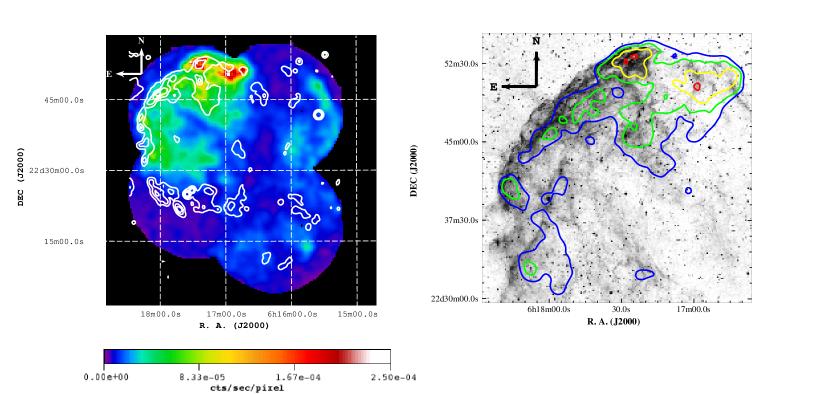
Figure 2.— Left panel: X-ray count rate image of IC443 in the 0.3–0.5 keV energy band. The image was adaptively smoothed using $\sigma_{min}$=10” and $\sigma_{max}$=40”; the bin size is 10”. We overlaid VLA NVSS contours at 1.4 GHz, corresponding to 5, 20, 45, 80 mJy beam^-1. Right panel: Optical DSS image of the northeastern shell of the remnant overlaid with contours of X-ray emission in the 0.3–0.5 keV energy band. Contour levels correspond to 1.7 (blue), 2.6 (green), 4.6 (yellow), 8.6 (red) 10^-3 cts s^-1 arcmin^-2.

2.2. Background subtraction

The EPIC MOS background components are mainly electronic noise, fluorescence emission lines (instrumental background, not vignetted), X-ray galactic emission (astrophysical background, vignetted) and soft magnetospheric protons focused by the optics (Lumb et al., 2002; Marty et al., 2003)

We removed high proton background time intervals by extracting light curves at energies $>8$ keV, where the EPIC cameras have a low quantum efficiency, with a bin time of 30 s . We rejected data intervals with more than 15 counts.

To check for a residual proton component we used a simple but useful diagnostic, developed by De Luca & Molendi (2004). We calculated for each screened data set the ratio R between the surface brightness in FOV ($\Sigma_{IN}$) and the surface brightness out FOV ($\Sigma_{OUT}$) in the energy range 8-12 keV. Following the definition given in De Luca & Molendi (2004), the maximum value of R, above which there is a significant soft proton contamination, is R_max=1.3. If 1.05$<$R$<$1.3 the residual proton level is low, if R$<$1.05 it can be considered negligible. We verified that our cleaned data sets have all a low or negligible residual proton component. After the screening process, the total exposure time was reduced by 25% (from 230 to 170 ks).

Table 1 summarizes the main information about the observation: the date, the pointing’s center coordinates, the exposure time before and after flare screening.

Instrumental background is the dominant component of the events out of FOV and it is also highly spatial variable. A typical solution is to estimate it using merged data sets acquired with the filter wheel in the CLOSED position (Lumb et al., 2002). We used the closed data sets of P. Marty, distributed by the School of Physics and Astronomy of the University of Birmingham.

Since IC443 is an extended source, that fills the entire field of view, it is not possible to estimate the local astrophysical background from the same data. Instead of a local background, we used a set of observations of blank sky regions, produced from the Galactic Plane Survey observations (GPS, P.I. Parmar), pointed toward a galactic longitude of 319^∘ and a galactic latitude between 0^∘ and 3^∘. This data set represents a better estimate of the cosmic background at low galactic latitude than the standard blank sky field at high $|b|$.
After the same screening process described in Sect. 2 and the removal of point sources, data sets were scaled by the relative exposure time and then reprojected onto the sky attitude of IC443 pointings with the script skycast.

From a comparison between the spectra extracted from the whole FOV of the CLOSED, GPS and IC443 data, we noted that in the energy range 0.3-5.0 keV the source signal is the brightest, while above 5.0 keV the instrumental noise component is the dominant one.
We decided to consider in our future analysis only events in the band 0.3–5.0 keV and to use GPS data as background correction. We verified that in this band our results are not sensitive to the background subtraction (either GPS or high galactic latitude blank fields).

3. Results

3.1. X-ray Images

We defined two energy bands, in which images has been extracted, so that in each band the contribution of a single component is the dominant one and, at the same time, the statistic data quality is good. In the chosen range 0.3–1.4 keV (soft band), the cold component flux (calculated assuming the parameters of the two components fit reported by Petre et al. 1988; Asaoka & Aschenbach 1994) is the 64% of the total; in the range 1.4–5.0 keV (hard band), the hot component flux represents the 90% of the total.
A third image, generated in the 0.3–0.5 keV band, traces the spatial distribution of the coldest X-ray emitting plasma and it is useful to trace the boundary between the SNR shock and the surrounding molecular clouds.

All the X-ray emission images presented here are background subtracted, exposure and vignetting corrected. To correct for the exposure and the vignetting, we divided the mosaiced background-subtracted count image by its mosaiced exposure map. The resultant image was adaptively smoothed with the SAS task asmooth.

Figure 1 shows the 4 pointings mosaiced image of IC443 in the 0.3–1.4 keV band. The brightest features are concentrated in the northeastern (NE) quadrant and a clear shell is not present. We mark a region near the rim of the remnant (filNE in Figure 1): the high surface brightness gradient suggests that we are looking the shock front nearly edge-on. The large effective area and the good spatial resolution of XMM-Newton allow us to have a better view of the western part of the remnant and to resolve its structure for the first time. Western X-ray emission appears about 10 times fainter and more diffuse than the eastern one. We can identify a bright filament (filNW in Fig. 1), that suggests the existence of a limb-brightened partial shell.
The arrows in Fig. 1 indicate two dark lanes, that cross the remnant: the first, from north to south, is probably due to the presence of a molecular cloud between the observer and IC443 (Petre et al., 1988); the second, from northeast to southwest, was explained by Asaoka & Aschenbach (1994) as an additional absorption effect by the SNR G189.6+3.3.

On the other hand, the morphology of the very soft emission (0.3–0.5 keV, see Fig. 2) is not centrally filled, the X-ray surface brightness peaks are near the northeastern edge of the remnant, resembling strikingly IC443 radio and optical emission. For comparison, we show in Fig. 2 (left panel) the X-ray image of the remnant in the 0.3–0.5 keV band, overlaid with contours of radio emission levels at 1.4 GHz, observed with the VLA NVSS survey (Condon et al., 1998). We also present the superposition between X-ray contours and the optical image, extracted from the DSS red survey (Lasker et al., 1990), of the northeastern quadrant of IC443, where it is encountering a H i cloud (Denoyer, 1978) (Fig. 2, right panel).
In the very soft X-ray band it is possible to resolve a partial shell structure in the NE, similar to that we see in the radio and optical images. Kawasaki et al. (2002) had already claimed the presence of a shell-like structure on the basis of ASCA GIS softness ratio map in the energy bands 0.7–1.5 and 1.5–10 keV. However our results represent a direct detection of a very soft shell, which is likely different from the structure reported by Kawasaki et al. (2002). In the light of our result on molecular cloud obscuration of the IC443 X-ray emission (see par. 4.3 below), we argue that the structure detected by Kawasaki et al. (2002) in their softness ratio map is due to the absorption of the foreground molecular cloud of Cornett et al. (1977) instead of a real shell morphology.

In the northeastern quadrant, radio, optical and very soft X-ray emission correlate well: X-ray brightest features are confined within the radio-optical shell and the position of maximum X-ray emission contour levels, just behind bright optical filaments, is in agreement with a shock front that has just encountered a density gradient of the ISM with higher density located in the outer regions. This correlation was also noted by Petre et al. (1988), which however focused only on the northern edge of the brightest soft X-ray region. Our results instead shows that this correlation involves the very soft X-ray shell and the optical-radio emission on a much greater extent.
The structures seen in the 0.3-0.5 keV map are of course affected by absorption, however we will see in sect.3.2 that the shape of the very soft shell is not correlated with the absorption map in the east of the SNR. In the light also of the good correlation between the very soft shell and the radio emission in the NE of IC443, we argue that a real shell structure exists.

In the southeastern quadrant, where the remnant is interacting with a dense molecular cloud, the spatial gap between X-ray emission and radio contours, as shown in Fig. 2, suggests that the shock front has been penetrated deeply inside the ring of molecular gas and it has been strongly decelerated, emitting mainly in the infrared band (Burton et al., 1988; Richter et al., 1995; Rho et al., 2001).

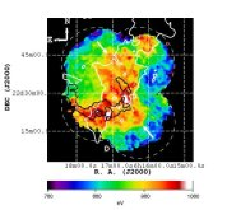
Figure 3.— Median energy map in the soft band (0.3–1.4 keV), overlaid with quiescent CO (white) and shocked H₂ (black) emission contours. The arrows indicate two high median energy regions without a counterpart in CO or H₂ maps. We masked some regions inside the observed field of view, traced by the dashed line, as they are too noisy (S/N$<$3). Image bin size is 20” and smoothing width is $\sigma$=20”. The velocity-integrated (-6 to 0 km s^-1) J=1–0 CO emission has 50” resolution. The velocity-integrated $v$=1–0 S(1) H₂ line emission at 2.122 $\mu$m has the spatial resolution of 40” (Burton et al., 1988).

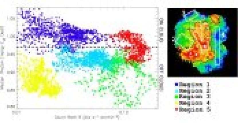
Figure 4.— Median/rate plot for the soft band (0.3–1.4 keV): on the Y-axis is reported the median photon energy, on the X- axis the corresponding count rate. The dashed line traces the median energy threshold at 0.97 keV between “on cloud” and “off cloud” regions. Points come from five regions, superimposed on the median energy map in the top right corner. The black contour in the map corresponds to the value of E₅₀=0.97 keV.

3.2. Median Energy Map

The complicated morphology of IC443 and the previous literature results suggest that the plasma has a distribution of physical conditions and so it is crucial to perform our spectral analysis selecting regions as homogeneous as possible. The median photon energy E₅₀ is a robust spectral indicator, as shown in Hong et al. (2004), that allows us to map spectral variations inside the field of view.

For a plasma in ionization equilibrium and with solar abundances (model MEKAL in XSPEC) we verified that in the soft band (0.3–1.4 keV) E₅₀ is mainly influenced by absorbing column variations, especially at large values of the absorption (N_H$\geq$0.5$\times$10²² cm^-2). The choice of the band assures that the median energy is not heavily affected by the parameters of the X-ray hot component.

Fig. 3 shows the median energy map of the emitting plasma in the 0.3–1.4 keV band. Molecular line data toward IC443 are plotted as contours over the image: quiescent CO in white (Lee J. J., private communication) and shocked H₂ in black (Burton et al., 1988).
To build the map we used a pixel size of 20”, in order to collect at least 10 photons per pixel, and then, for each pixel we calculated the median photon energy. The resulting image was smoothed using a bidimensional Gaussian distribution with $\sigma$=20”. No correction for the X-ray background was made, we simply masked faint regions, where the signal to noise ratio was less than 3.
The image presented in Fig. 3 allows us to compare spectral properties of the cold X-ray component with the emission of shocked and quiescent molecular gas with an unprecedented spatial resolution (28”, corresponding at $\sim$0.2 pc at a distance of 1.5 kpc).
Previous studies about IC443 (Petre et al., 1988; Asaoka & Aschenbach, 1994) tried to link spectral hardness ratio variations across the remnant to an absorption effect, but the low images resolution did not permit to study the correlation with the molecular cloud material on small angular scales. Moreover, previous hardness ratio maps are sensitive both to absorption effects and to the parameters of the hot component, whereas our median energy map is more strongly dependent on absorption.
The spatial variations of the spectral properties reported in our map (Fig.3) confirm the distribution of the hardness ratio in Asaoka & Aschenbach (1994), but shows more details. In particular, we find a strict correlation, also on small angular scales, between molecular emission contours and high median energy regions, as expected in the case of an increasing column density. They match very well everywhere, except two high median regions, indicated by the arrows in Fig. 3, that seems not to have a counterpart in CO and H₂ maps.

As already shown in the study of the Vela supernova remnant of Miceli et al. (2005), the relation between the median photon energy E₅₀ and the corresponding count rate R in each pixel is able to give a global view of different thermal structures and spectral variations inside the field of view, preliminary to a complete spectral analysis. As shown in Fig. 4, we selected five significant regions and made the corresponding E₅₀ vs. R plot to get further information about the physical parameters of the plasma. We applied the Maritz-Jarrett method to estimate the errors on the median energy, as described by Hong et al. (2004), and we assumed a poissonian error for the count rate values. In order to avoid excessive noise, especially in faint areas, points with $\sigma(E_{50})\geq$5% or $\sigma(R)\geq$15% were not reported in the plot.

It is worth to note that all the points belonging to region 1 (blue circles), which corresponds to a CO emission area, have the highest median values (E${}_{50}\geq$1.0 keV), while points from other regions lie below this energy threshold. In particular, we can distinguish two distinct branches at 1.0 keV (region 1) and at 0.9 keV (region 2 and a great part of region 3). These features could be interpreted as an absorption effect: on average plasma physical conditions appear to be the same in different regions, the only difference being an increase of the column density, that shift points from region 1 towards higher median and lower rate values. We may define the boundary of off-cloud and on-cloud regions with the value E₅₀=0.97 keV (dashed line in Fig. 4, left panel), whose contour is also reported in the right panel of Fig. 4. Data from the off-cloud region 4 (yellow diamonds) are those affected by the greatest uncertainties. They show similar E₅₀ values of region 3 (green squares), but seem isolated from the others, maybe suggesting physical differences, e.g. a lower interstellar absorption. The arc-like shape, identified by region 5 red points, is characteristic of temperature variations for a plasma in pressure equilibrium (Miceli et al., 2005). It seems also present in the off-cloud region 3, though less evident.

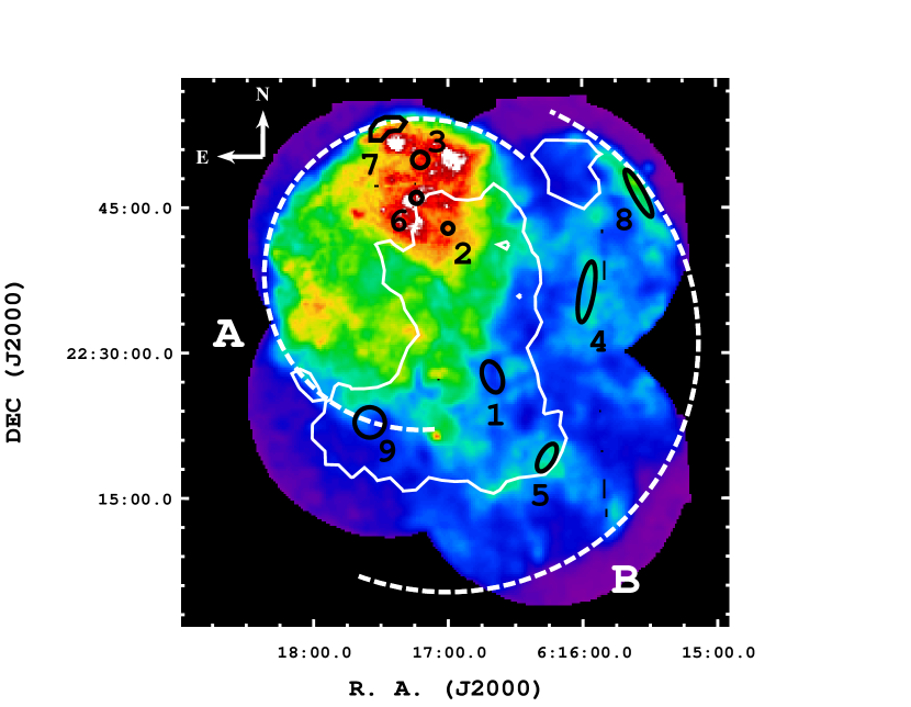
Figure 5.— X-ray count rate image of IC443 in the 0.3–1.4 keV energy band, on which we superimposed the nine regions selected for spectral analysis and the median photon energy contour (white) corresponding to E₅₀=0.97 keV. The dashed semicircles mark subshell A and subshell B structures. The color bar is the same as in Fig. 1.

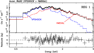
Figure 6.— XMM-Newton EPIC MOS spectra representative of IC443 thermal emission. The top figure shows the spectrum of reg 1 with the corresponding two components best fit model and, in the lower panel, the residuals distribution. The blue dashed line represents the cold spectral component, while the red dotted line represents the hot one. The bottom figure shows the spectrum of reg 8 with its corresponding single component best fit model and, in the lower panel, the residuals distribution.

Table 2Dimensions, counts and best-fit parameter values for the nine spectral regions. For each spectrum we also report the derived filling factor for each spectral component. Quantities in square brackets are held fixed at the given value. All the reported errors are at the 90% confidence level.

Parameters	Reg 1	Reg 2	Reg 3	Reg 4	Reg 5	Reg 6	Reg 7	Reg 8	Reg 9
Area (arcmin2)	5.2	1.1	2.2	7.5	2.3	1.1	5.5	5.0	7.1
Counts (103)	5.6	6.9	5.9	5.8	6.3	7.0	4.6	4.8	6.7
NH (1022 cm-2)	0.96${}_{-0.2}^{+0.17}$	0.74${}_{-0.13}^{+0.11}$	0.56${}_{-0.10}^{+0.12}$	0.43${}_{-0.03}^{+0.06}$	0.45${}_{-0.05}^{+0.05}$	0.64${}_{-0.06}^{+0.07}$	0.57${}_{-0.16}^{+0.12}$	0.58${}_{-0.07}^{+0.07}$	0.64${}_{-0.13}^{+0.16}$
Cold component
kTs (keV)	0.37${}_{-0.04}^{+0.07}$	0.58${}_{-0.04}^{+0.03}$	0.29${}_{-0.03}^{+0.02}$	0.31${}_{-0.03}^{+0.06}$	0.64${}_{-0.04}^{+0.04}$	0.358${}_{-0.012}^{+0.020}$	0.29${}_{-0.06}^{+0.07}$	0.31${}_{-0.04}^{+0.07}$	0.66${}_{-0.07}^{+0.06}$
$\tau$ (1012 cm-3 s)	48 ($\geq$2)	2.0${}_{-1.2}^{+5}$	50 ($\geq$2)	2.3 ($\geq$0.7)	CIE	50 ($\geq$3.3)	0.21${}_{-0.10}^{+0.8}$	1.0${}_{-0.7}^{+9}$	1.2${}_{-0.8}^{+3}$
$F_{s}$	4${}_{-3}^{+4}$	6$\pm 3$	11${}_{-7}^{+20}$	8$\pm 4$	2.3$\pm 0.8$	7.0${}_{-2}^{+1.8}$	16${}_{-9}^{+30}$	70${}_{-30}^{+50}$	2,1$\pm 1,8$
O/O⊙	[ 1 ]	4.3${}_{-1.6}^{+4}$	1.3${}_{-0.7}^{+3}$	0.44${}_{-0.10}^{+0.17}$	2.6${}_{-1.0}^{+2}$	0.8${}_{-0.3}^{+0.5}$	0.8${}_{-0.3}^{+0.5}$	0.52${}_{-0.16}^{+0.3}$	[ 1 ]
Ne/Ne⊙	1.9${}_{-1.0}^{+8}$	3.5${}_{-1.2}^{+2}$	1.2${}_{-0.6}^{+4}$	0.45${}_{-0.11}^{+0.16}$	2.8${}_{-0.9}^{+1.9}$	1.0${}_{-0.3}^{+0.5}$	0.9${}_{-0.2}^{+0.3}$	0.7${}_{-0.2}^{+0.4}$	2.6${}_{-0.9}^{+6}$
Mg/Mg⊙	1.0${}_{-0.5}^{+6}$	1.3${}_{-0.3}^{+0.8}$	0.7${}_{-0.4}^{+0.2}$	0.32${}_{-0.11}^{+0.16}$	1.5$\pm 0.5$	0.48${}_{-0.12}^{+0.2}$	0.6${}_{-0.2}^{+0.3}$	0.50${}_{-0.17}^{+0.3}$	1.4${}_{-0.5}^{+6}$
Si/Si⊙	[ 1 ]	[ 1 ]	[ 1 ]	[ 1 ]	0.4${}_{-0.16}^{+0.2}$	[ 1 ]	1.1${}_{-0.6}^{+1.4}$	0.5${}_{-0.3}^{+0.5}$	[ 1 ]
S/S⊙	[ 1 ]	[ 1 ]	[ 1 ]	[ 1 ]	0.13 ($\leq$0.4)	[ 1 ]	[ 1 ]	[ 1 ]	[ 1 ]
Fe/Fe⊙	0.4${}_{-0.2}^{+1.3}$	0.9${}_{-0.4}^{+0.8}$	1.3${}_{-0.6}^{+3}$	0.32${}_{-0.06}^{+0.09}$	0.15${}_{-0.06}^{+0.13}$	0.51${}_{-0.14}^{+0.3}$	0.8$\pm 0.2$	0.45${}_{-0.11}^{+0.2}$	0.5${}_{-0.2}^{+1.6}$
filling factor $f_{s}$	0.15	0.42	0.26	1.0	1.0	0.52	1.0	1.0	0.2
Hot component
kTh (keV)	1.11${}_{-0.16}^{+0.3}$	1.78${}_{-0.18}^{+0.13}$	1.01${}_{-0.06}^{+0.13}$	—	—	1.4${}_{-0.3}^{+0.8}$	—	—	1.73${}_{-0.13}^{+0.19}$
$F_{h}$	1.4${}_{-0.7}^{+0.8}$	0.43${}_{-0.16}^{+0.6}$	1.8${}_{-1.2}^{+0.8}$	—	—	0.42${}_{-0.19}^{+0.3}$	—	—	0.8${}_{-0.6}^{+0.5}$
Mg/Mg⊙	2.3${}_{-1.1}^{+4}$	$>$5	0.8${}_{-0.6}^{+0.8}$	—	—	$\geq$2	—	—	$\geq$4
Si/Si⊙	0.5$\pm 0.3$	$\geq$3	1.0$\pm 0.5$	—	—	$\geq$5	—	—	1.7${}_{-0.6}^{+5}$
S/S⊙	0.7${}_{-0.3}^{+0.7}$	$\geq$3	1.0$\pm 0.6$	—	—	$\geq$3	—	—	1.3${}_{-0.5}^{+2}$
Fe/Fe⊙	$\leq$0.06	$\leq$1.3	0.5${}_{-0.3}^{+0.4}$	—	—	$\leq$1.2	—	—	$\leq$0.07
filling factor $f_{h}$	0.85	0.58	0.74	—	—	0.74	—	—	0.8
$\chi^{2}$/dof	152/150	147/125	98/85	76/89	129/96	151/121	103/79	113/99	119/116

3.3. Spectral Analysis

The XMM-Newton data allowed us to significantly improve the spatial resolution of the spectral analysis with respect to past works about IC443 (Petre et al., 1988; Kawasaki et al., 2002).
We analyzed spectra extracted from the regions marked in Fig. 5. These regions were selected so as to represent the main features of the cold plasma, as obtained from imaging analysis. We focused on the following aspects: (a) to verify the presence of a column density gradient across the FOV and its correspondence with median photon energy variations (regions 1–5); (b) to characterize physically the partial shell structure (regions 7 and 8) and the site of interaction with the molecular ring (region 9); (c) to probe the ISM properties in the northeastern quadrant, where the surface brightness has its peaks (regions 2, 3, 6 and 7), and in the western one, never studied before (regions 4, 5 and 8).
Regions shapes and sizes were determined on the basis of statistical and homogeneity criteria so as to have minimum $\sim$5000 counts and small fluctuations of the median photon energy ($<$5%).

Before performing our analysis, we corrected for the vignetting effect assigning a weight to each event (task evigweight) and then we extracted source and background spectra from the new events list. This procedure changes the spectral shape of the instrumental background, which is not vignetted, so it is necessary to extract background spectra in the same regions as the observed source data. For fitting we used the sum of MOS1 and MOS2 spectra, the average of on-axis ARFs, weighted for the instruments exposure time, and the MOS1 canned response matrix m1_110_im_pall_v1.2.rmf. The spectra were grouped with a minimum of 25 counts per bin and the $\chi^{2}$ statistic was used. We first applied a single thermal component model, testing both for ionization non-equilibrium (VPSHOCK, Borkowski et al. 2001) and equilibrium (VMEKAL) cases, and, when needed, we added a second thermal component to achieve a good fit. We left free to vary O, Ne, Mg and Fe abundances of the cold component and Mg, Si, S and Fe abundances of the hot component. The two components fits with linked abundances give worse results than the fits with indipendent abundances.

Figure 6 shows two representative spectra, extracted from regions 1 and 8, with their corresponding best fit models and residuals. Best fit parameters of all the analyzed regions are presented in Table 2 with the corresponding errors at the 90% confidence limit (Lampton et al., 1976).
In the eastern part (regions 1,2,3,6 and 9 in Table 2) IC443 thermal emission in the 0.3–5.0 keV band can be generally described with a two temperature model: the colder (kT$\sim$0.3 keV) is characterized by solar abundances (Anders & Grevesse, 1989) and a ionization timescale $\tau\geq$10¹² cm^-3 s^-1, very close to equilibrium conditions, the hotter (kT$\geq$1.0 keV) by overabundant Mg, Si and S and ion equilibrium. On the other side, we found the spectra from western regions (number 4,5 and 8 in Table 2) to be adequately modeled by a single soft component.

The reduced $\chi^{2}$ probability is above 5% for all regions, except for region 5 and 9, where we have $\chi^{2}$_ν=1.3 (1.3%) and $\chi^{2}$_ν=1.2 (3%).

4. Discussion

4.1. Global properties of the X-ray emitting cold plasma

The soft X-ray emission of IC443 shows high values of ionization timescale and a normal chemical composition, which suggests an origin from shocked dense circumstellar or ISM material.

Previous works about IC443 had left some ambiguity on the plasma ionization state. The work of Petre et al. (1988), based on Einstein data, was not able to discriminate between equilibrium and non equilibrium ionization scenarios. Afterward, the analysis of ROSAT observations, made by Asaoka & Aschenbach (1994), described the X-ray emission with a two temperatures ($\sim$0.3 and $\sim$1.0 keV) Raymond-Smith model, but the data resolution did not allow to check for the presence of non-equilibrium conditions. On the basis of ASCA data, Kawasaki et al. (2002) suggested a high degree of non-equilibrium ($\tau$$\sim$10¹¹ cm^-3 s) to explain the soft X-ray thermal structure of IC443 in its NE quadrant.
The temperature obtained in the selected regions are generally in agreement with the results of the “pure IC443” regions of Asaoka & Aschenbach (1994). Moreover, unlike Kawasaki et al. (2002) our spectral results give a soft X-ray component near the equilibrium condition ($\tau$$\sim$10¹² cm^-3 s) for all regions except region 7, in which we have $\tau$$\sim$10¹¹ cm^-3 s. The hot component is fully equilibrated.

To infer important values of the gas parameters, such as the mean electron density and the total mass of the shocked ISM, we assumed a shell-like morphology and typical cosmic abundances ($n_{e}$$\sim$1.2 $n_{H}$) for the soft component. We took into account IC443 double shell structure, so we approximated the X-ray emitting volume $V$ as two hemispheres with radii R_A=16’ ($\sim$7 pc) for the eastern side (subshell A in Fig. 5) and R_B=26’ ($\sim$11 pc) for the western side (subshell B in Fig. 5), following the results of Braun & Strom (1986) and Chevalier (1999).

The electron density is thus given by $n_{e}^{2}\sim{\rm EM}_{s}$/ (1.2$f_{s}V$), where EM_s and $f_{s}$ are the emission measure and the soft component filling factor.
For those regions in which we resolved only a soft thermal component, the standard shell geometry was adopted: we assumed that the emitting plasma is confined in a thin shell with a thickness of $\sim$1 pc. To evaluate the filling factors of the other regions we made the assumption of pressure equilibrium between the soft and the hard component ($n_{s}T_{s}$$\sim$$n_{h}T_{h}$), deriving $f_{s}^{-1}$=1+(EM_h/EM_s)(T_h/T_s)² (see e.g. Bocchino et al. 1999). The derived filling factor values are listed in Tab. 2.

Fig. 7 shows electron densities and temperatures for each spectral region with the corresponding 90% error bars. Regions are plotted in order of distance from the PWNe.
Subshell B mean density, with a value of $\sim$1 cm^-3, appears homogeneous. In subshell A regions nearest to the rim (reg 7, 3, 6) there is an indication of a density factor two times larger than in the other regions. This is consistent with an outwardly increasing density profile near the rim, which points toward the region of the bright very soft shell and optical filaments.
These results can be explained consistently with a shock which is expanding in a homogeneous and low density environment in the west, while it has been decelerated by the encounter with a density gradient in the east, located in a thin region of $\sim$4 pc near the rim.

We made a rough estimation of the total soft X-ray emitting mass taking for each subshell the average of the density values, $<n>_{A}$ and $<n>_{B}$, and assuming that the blast wave shell is 2’ thick. We found M_X$\sim$30 M_⊙, which is a small fraction of the predicted mass of the dense molecular cloud (M$\lesssim$10⁴ M_⊙, Cornett et al. 1977) and the H i cloud (M$\sim$10²-10³ M_⊙, Denoyer 1978). This is reasonable, also in the light of our results about the presence of a density gradient through most of the IC443 rim (see sect. 4.2), since the material emitting in the X-rays is just the outskirts of large clouds.

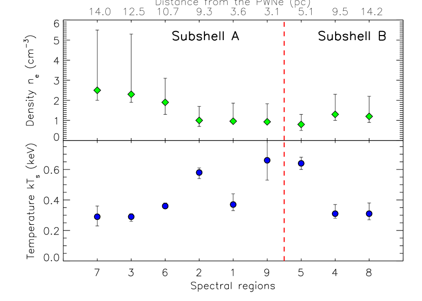
Figure 7.— Electron mean density n_e (top panel) and temperature kT_s (bottom panel) of the cold X-ray emitting plasma in the nine spectral regions indicated on the X-axis. The density values were derived from spectral analysis as the square root of the emission measure divided by 1.2 times the volume occupied by the cold plasma. Subshell A regions (on the left of the vertical dashed line) and subshell B regions (on the right of the vertical dashed line) are plotted in order of distance from the PWNe.

4.2. Interaction with the environment

We further investigated the evolutionary stage of the X-ray emitting mass in the region between the remnant and the molecular clouds, in order to pinpoint possible effects of the interaction with these large structures. In Fig. 8, we display $\chi^{2}$ contours in the ionization time $\tau$ vs. emission measure EM_s space for three regions located in sites of putative strong interaction of the remnant with the environment, namely region 7 (interaction with the neutral clouds), 8 (interaction with ISM) and 9 (interaction with the southern molecular ring). We also show the post-shock electron density $n_{e}$ and the age of the emitting plasma computed using the relation $\tau=n_{e}t$, where $t$ is the time since the passage of the shock and $n_{e}$ is assumed constant after the shock. The age calculated in this way is a very rough estimate and it is more useful for comparing different regions than for the evaluation of the true age.

We stress that for all the regions, the ionization time values are compatible with collisional ionization equilibrium (CIE) at the $3\sigma$ level. However, we note that region 7 has a best-fit ionization time which is $\sim 5$ times lower than 8 and 9 and an age value which is 10 times lower, thus opening the possibility that the plasma was more recently hit at NE. This is in agreement with a location for the SN near the current position of the pulsar wind nebula (PWNe), which is also supported by the higher values of kT_s for the regions near the PWNe (e.g. regions 1, 5, 9) than for the regions far from it (e.g. regions 6, 7, 8). According to this interpretation, therefore, the regions near the explosion are hotter and more evolved than the regions far from it, because they were shocked at higher speed long time ago. From this point of view, however, it is difficult to explain why the two fronts regions (7 in NE and 8 in NW) have also different best-fit values for ionization time and age, since they are probably located at the similar distances from the explosion site.

From the condition $\rho$v²=constant, we derived an independent estimate of the evolutionary age of region 7. The shock velocity corresponding to plasma temperatures of 0.3 keV is v_sh$\sim$450 km s^-1. The density of the X-ray emitting plasma that we have calculated is 2.5 cm^-3. For the H i cloud we took density and velocity values from the literature: $n$$\sim$10 cm^-3 and v$\sim$100 km s^-1 (Rho et al., 2001). Optical and X-ray brightness peaks are 23”(2 pc) far apart, so we assumed an exponential density distribution with a scale height of 0.15 pc. The time elapsed since the shock front has encountered the cloud is thus $\sim$2$\times$10³ yr, in agreement with the hypothesis of a recent interaction.

Alternatively, the low ionization time of region 7 can be explained by the fact that the extraction region includes plasma at very different densities (e.g. in case of strong density gradient). In this case it is possible that the VPSHOCK models used in the fit try to reproduce the coldest plasma with a low ionization scale. In fact, we have seen in Fig. 7 that the density in this region increases by a factor of 2.5 in 5 pc (from $n_{e}\sim$1 in reg 1 to $n_{e}\sim$2.5 in reg 7), and that there is an additional compression of a factor of $\sim$4 in 2 pc between the X-ray and optical filaments, so this interpretation is realistic.

A more accurate estimate of the ionization age in both regions 7 and 8 would need more data.

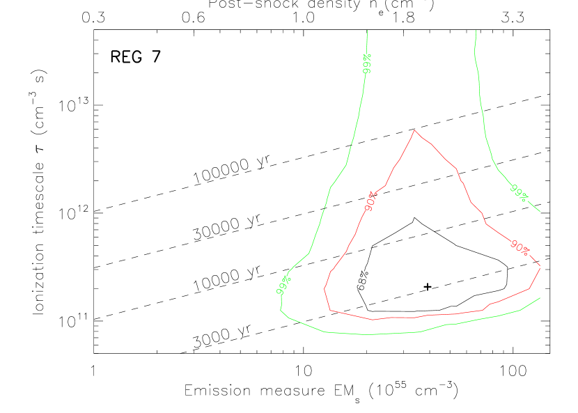
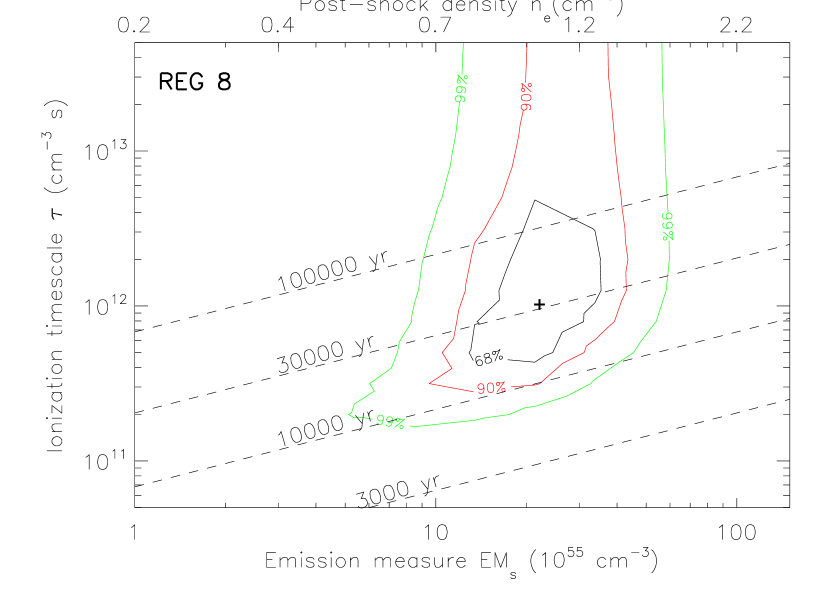
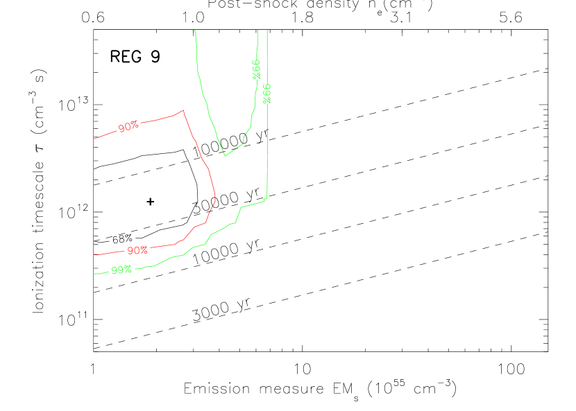
Figure 8.— Confidence level $\chi^{2}$ contours (68%, 90% and 99%) in the EM_soft-$\tau$ parameter space for three spectral regions (7, 8 and 9). On the top X-axis are reported the corresponding post-shock electron densities. We show the range of ages which are compatible with the values derived from the fit.

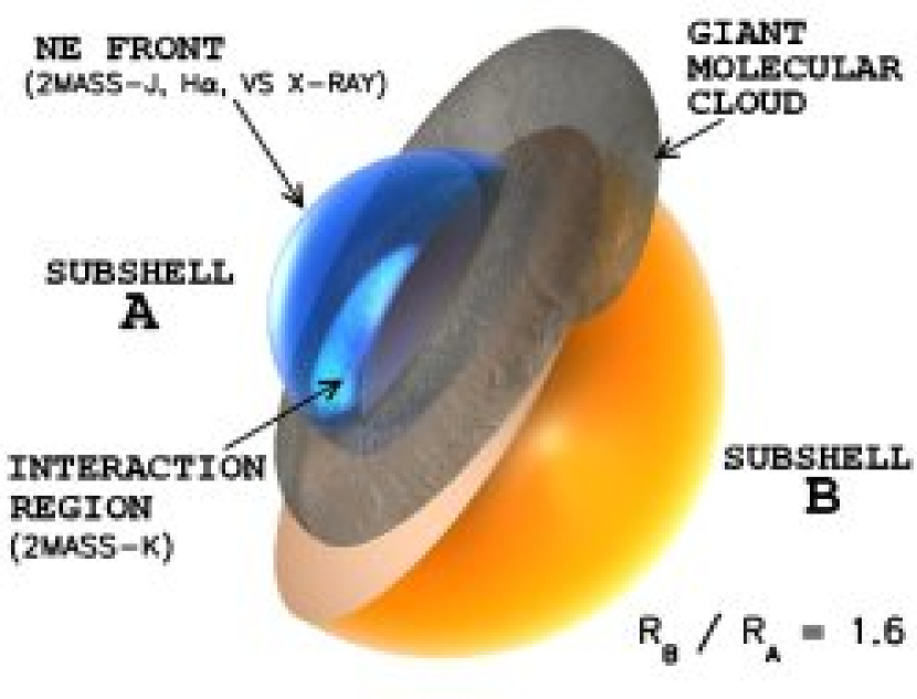
Figure 9.— Two-shells model describing IC443 morphology. The dark ring represents the giant molecular cloud of Cornett et al. (1977). The blue hemisphere, labelled as subshell A, represents the shock front in the eastern region. In the north-east, where it has been confined by the encounter with the neutral H i cloud of Denoyer (1978), the shock front is traced by optical, infrared (2MASS-J energy band) and very soft X-ray (0.3–0.5 keV energy band) emission. In the south-east the light blue strip indicates the region of interaction with the molecular cloud, which instead is bright in the 2MASS-K energy band (Rho et al., 2001). The orange hemisphere, labelled as subshell B, represents the shock front in the western region, where it is expanding in a homogeneous and less dense medium. The ratio of the shells radii is 1.6, as derived by our X-ray images.

4.3. Absorption from molecular clouds

The spatial overlap in the image plane between high median energy values and molecular emission, shown in Fig. 4, together with the median/count rate relation suggest an increase of the foreground absorption in the direction of CO and H₂ emission.

Using the median photon energy as a spectral indicator, we selected five representative regions (1, 2, 3, 4 and 5 in Fig. 5) to study temperature and column density distribution across the FOV. Our best fit results are plotted in Fig. 10 with the corresponding error bars at the 90% confidence level.
They confirm that higher N_H values correspond to higher median energies and identify an increasing trend of the column density. Moreover, the best fit absorbing column of region 1 is significantly higher than the mean Galactic absorption toward this portion of sky (N${}_{\rm H}^{\rm Gal}\sim$ 6.3$\times$10²¹ cm^-2, Dickey & Lockman 1990), indicating the presence of additional absorbing material. We estimate that it contributes an equivalent column density of $\Delta$N_H$\sim$5$\times$10²¹ cm^-2. The spatial distribution of the obscuring material and the corresponding N_H values point to the identification with the unperturbed cloud of Cornett et al. (1977). Our X-ray data strongly suggest that it is located in front of IC443, between the remnant and the observer.

The southern sinuous ridge shows the same E₅₀ values of the quiescent cloud, indicating similar hydrogen column density. In the median energy map of Fig. 3, the southern ridge and the quiescent cloud appear as a single complex. We argue that both probably belong to the same cloud structure, which has been reached by the IC443 shock in several location of the south side (corresponding to clump A to G of Dickman et al. 1992), while it is mostly unshocked elsewhere, in particular in the on-cloud regions (Fig. 3) where there is no maser or H₂ infrared emission. Dickman et al. (1992) suggested that the shocked material is in a $\sim$9$\times$7 pc ring tilted by $\sim$50^o from the line of sight and that it is expanding, presumably as a result of the interaction. We expand this picture by arguing that the Dickman ring represents only the shocked part of a large molecular cloud complex shaped as a large tilted torus, which is obscuring the background SNR X-ray emission.

In Fig. 9 we show the proposed model for the environments of IC443. This model is supported by the comparison (see Fig. 3) between our median energy image and the contour of Burton et al. (1988), which traces the boundaries of the shocked gas, and the CO contours indicating quiescent dense material. While the southern and western on-cloud regions are characterized by high median energy values (E₅₀$>$0.98 keV), which locate the molecular ring in the foreground, the northeastern regions have E₅₀$\sim$0.9 keV, indicating lower extinction and thus, suggesting that the large torus lies in the background, as expected in the case of a tilted geometry encompassing the whole SNR. This picture is in agreement with kinematic velocities measured in clumps A to H by Dickman et al. (1992), and by the more recent study of clump H and H₂ infrared emission of Rho et al. (2001). In particular, the latter authors detect weak 2MASS-K filaments in a region called “NE front”, which includes clump H and is separated from the bright optical and radio NE rim. They argue that the clump H/NE front region is part of the molecular cloud interaction, as the sinuous southern ridge, and the fact that it is an “off-cloud” region according to our Fig. 10 suggests that it represents the interaction of the SNR shock with the part of the torus lying behind the SNR.

The comparison between the 0.3–0.5 keV map (Fig. 2) and the median energy map (Fig. 3) shows that the very soft shell is not correlated with absorption in the east of the remnant, thus indicating that this shell is not entirely an effect of absorption.

The median energy map allowed us to investigate the issue of the location of the nearby SNR G189.6+3.3. This remnant was located by Asaoka & Aschenbach (1994) in front of IC443, causing a dark lane of absorption equivalent to $\Delta$N_H$\sim$2$\times$10²¹ cm^-2. This would raise the value of the median energy of $\Delta$E₅₀$\sim$80 eV. Our results does not support strong absorption from the shell of G189.6+3.3. We conclude that either its contribution to N_H should be small compared to that of the CO cloud or the SNR could be in the background.

Finally, from the spectral results presented in Table 2, we argue that the peculiar location of region 5 in the temperature vs. median energy plot (Fig. 10, lower panel) is an effect of high temperature rather than column density. This is expected, since for N_H$<$ 5$\times$10²¹ cm^-2 our median energy map is more sensitive to temperature variations than for higher N_Hvalues.

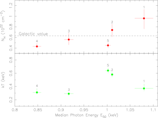
Figure 10.— Column density N_H (top panel) and electron temperature k_BT (bottom panel) vs. the median photon energy of the indicated spectral regions.The dashed line in the top panel indicate the absorption column mean value toward IC443 direction.

5. Conclusions

We presented results from XMM-Newton observations of the Galactic SNR IC443. High resolution image in the 0.3-0.5 keV energy band unveils a partial limb-brightened X-ray shell, which resembles on small angular scales the optical and radio morphology in the NE quadrant and which is different from the shell structure previously reported by Kawasaki et al. (2002). We concluded that it spatially traces the interaction of the shock with a density gradient, which is part of the neutral northeastern cloud studied by Denoyer (1978).

The spatially resolved spectral analysis of IC443 measured large column density variations across the remnant, and the median photon energy distribution shows that they are spatially coincident with molecular emission from dense molecular clouds in the FOV. Our results confirmed that X-ray emission is strongly absorbed by the molecular cloud of Cornett et al. (1977) and by the southern sinuous ridge of Burton et al. (1988). We did not find evidence of absorption from the SNR G189.6+3.3.
On the basis of our median energy map, we proposed that the southern ring and the more extended molecular cloud are part of the same structure and that it is tilted respect to the line of sight, as suggested by Dickman et al. (1992).

We performed spectral analysis in 9 bright regions with at least 5000 counts and a 5% maximum variation of the median photon energy E₅₀. The X-ray emission from our selected regions is well described with CIE or near ionization equilibrium models. Our measured X-ray temperatures and ionization timescales are compatible with a density gradient in the NE rim and suggest that the site of the SN explosion could be near the PWNe.

References

- Anders & Grevesse (1989) Anders, E. & Grevesse, N. 1989, Geochim. Cosmochim. Acta, 53, 197
- Arnaud (1996) Arnaud, K. A. 1996, in ASP Conf. Ser. 101: Astronomical Data Analysis Software and Systems V, 17–+
- Asaoka & Aschenbach (1994) Asaoka, I. & Aschenbach, B. 1994, A&A, 284, 573
- Bocchino & Bykov (2000) Bocchino, F. & Bykov, A. M. 2000, A&A, 362, L29
- Bocchino & Bykov (2001) Bocchino, F. & Bykov, A. M. 2001, A&A, 376, 248
- Bocchino & Bykov (2003) Bocchino, F. & Bykov, A. M. 2003, A&A, 400, 203
- Bocchino et al. (1999) Bocchino, F., Maggio, A., & Sciortino, S. 1999, A&A, 342, 839
- Braun & Strom (1986) Braun, R. & Strom, R. G. 1986, A&A, 164, 193
- Burton et al. (1988) Burton, M. G., Geballe, T. R., Brand, P. W. J. L., & Webster, A. S. 1988, MNRAS, 231, 617
- Chevalier (1999) Chevalier, R. A. 1999, ApJ, 511, 798
- Claussen et al. (1997) Claussen, M. J., Frail, D. A., Goss, W. M., & Gaume, R. A. 1997, ApJ, 489, 143
- Condon et al. (1998) Condon, J. J., Cotton, W. D., Greisen, E. W., et al. 1998, AJ, 115, 1693
- Cornett et al. (1977) Cornett, R. H., Chin, G., & Knapp, G. R. 1977, A&A, 54, 889
- De Luca & Molendi (2004) De Luca, A. & Molendi, S. 2004, A&A, 419, 837
- Denoyer (1978) Denoyer, L. K. 1978, MNRAS, 183, 187
- Dickey & Lockman (1990) Dickey, J. M. & Lockman, F. J. 1990, ARA&A, 28, 215
- Dickman et al. (1992) Dickman, R. L., Snell, R. L., Ziurys, L. M., & Huang, Y.-L. 1992, ApJ, 400, 203
- Esposito et al. (1996) Esposito, J. A., Sreekumar, P., Hunter, S. D., & Kanbach, G. 1996, Bulletin of the American Astronomical Society, 28, 1346
- Hoffman et al. (2003) Hoffman, I. M., Goss, W. M., Brogan, C. L., Claussen, M. J., & Richards, A. M. S. 2003, ApJ, 583, 272
- Hong et al. (2004) Hong, J., Schlegel, E. M., & Grindlay, J. E. 2004, ApJ, 614, 508
- Kawasaki et al. (2002) Kawasaki, M. T., Ozaki, M., Nagase, F., et al. 2002, ApJ, 572, 897
- Keohane et al. (1997) Keohane, J. W., Petre, R., Gotthelf, E. V., Ozaki, M., & Koyama, K. 1997, ApJ, 484, 350
- Lampton et al. (1976) Lampton, M., Margon, B., & Bowyer, S. 1976, ApJ, 208, 177
- Lasker et al. (1990) Lasker, B. M., Sturch, C. R., McLean, B. J., et al. 1990, AJ, 99, 2019
- Lumb et al. (2002) Lumb, D. H., Warwick, R. S., Page, M., & De Luca, A. 2002, A&A, 389, 93
- Marty et al. (2003) Marty, P. B., Kneib, J.-P., Sadat, R., Ebeling, H., & Smail, I. 2003, in X-Ray and Gamma-Ray Telescopes and Instruments for Astronomy. Edited by Joachim E. Truemper, Harvey D. Tananbaum. Proceedings of the SPIE, Volume 4851, pp. 208-222 (2003)., 208–222
- Miceli et al. (2005) Miceli, M., Bocchino, F., Maggio, A., & Reale, F. 2005, A&A, 442, 513
- Olbert et al. (2001) Olbert, C. M., Clearfield, C. R., Williams, N. E., Keohane, J. W., & Frail, D. A. 2001, ApJ, 554, L205
- Petre et al. (1988) Petre, R., Szymkowiak, A. E., Seward, F. D., & Willingale, R. 1988, ApJ, 335, 215
- Rho et al. (2001) Rho, J., Jarrett, T. H., Cutri, R. M., & Reach, W. T. 2001, ApJ, 547, 885
- Rho & Petre (1998) Rho, J. & Petre, R. 1998, ApJ, 503, L167
- Richter et al. (1995) Richter, M. J., Graham, J. R., & Wright, G. S. 1995, ApJ, 454, 277
- Sturner et al. (2004) Sturner, S. J., Keohane, J. W., & Reimer, O. 2004, Advances in Space Research, 33, 429
- Turner et al. (2001) Turner, M. J. L., Abbey, A., Arnaud, M., et al. 2001, A&A, 365, L27
- van Dishoeck et al. (1993) van Dishoeck, E. F., Jansen, D. J., & Phillips, T. G. 1993, A&A, 279, 541
- Wang et al. (1992) Wang, Z. R., Asaoka, I., Hayakawa, S., & Koyama, K. 1992, PASJ, 44, 303
- Welsh & Sallmen (2003) Welsh, B. Y. & Sallmen, S. 2003, A&A, 408, 545