Optical Polarimetry of the Jets of Nearby Radio Galaxies: I. The Data

Abstract

In this paper, the first in a series, we present an overview of new Hubble Space Telescope (HST) imaging polarimetry of six nearby radio galaxies (3C 15, 3C 66B, 3C 78, 3C 264, 3C 346, and 3C 371) with optical jets. These observations triple the number of extragalactic jets with subarcsecond-resolution optical polarimetry. We discuss the polarization characteristics of each jet and, as our Stokes I images also represent by far the deepest optical images yet obtained of each of these jets, we also discuss the morphology in total flux of each jet in detail. We find evidence of high optical polarization, averaging $20\%$, but reaching upwards of $\sim 50\%$ in some objects, confirming that the optical emission is synchrotron, and that the components of the magnetic fields perpendicular to the line of sight are well ordered. We find a wide range of polarization morphologies, with each jet having a somewhat different relationship between total intensity and polarized flux and the polarization position angle. We find two trends in all of these jets. First, jet “edges” are very often associated with high fractional optical polarizations, as also found in earlier radio observations of these and other radio jets. In these regions, the magnetic field vectors appear to track the jet direction, even at bends, where we see particularly high fractional polarizations. This indicates a strong link between the local magnetic field and jet dynamics. Second, optical flux maximum regions are usually well separated from maxima in fractional polarization and often are associated with polarization minima. This trend is not found in radio data and was found in our optical polarimetry of M87 with HST. However, unlike in M87, we do not find a general trend for near-90^∘ rotations in the optical polarization vectors near flux maxima. We discuss possibilities for interpreting these trends, as well as implications for jet dynamics, magnetic field structure and particle acceleration.

1 Introduction

Relativistic jets have been known for many years as a hallmark of powerful extragalactic radio sources. The compilation of Liu & Zhang (2002) listed over 660 sources with known, resolved radio jets, as of December 2000. The number of optical and X-ray jets is far smaller: about three dozen are known in each band (see the WWW pages maintained by Harris (XJET; Harris 2003) and Jester (Jester et al. 2004) respectively for lists of confirmed X-ray and optical jets). This does not signify a paucity of optical and X-ray emission, but instead, reflects the fact that few comprehensive surveys for jets have been done in those bands. Indeed, until the advent of the Hubble Space Telescope (HST) and Chandra X-ray Observatory, no survey had been done which was reasonably optimized for the detection of jets. Even now, there have been few HST surveys for jets: the largest, the 3CR snapshot surveys (optical: de Koff et al. 1996, Martel et al. 1999; UV: Allen et al. 2002; near-IR: Madrid et al. 2006), includes more than 100 objects (not all of which have radio jets), but is complete only to $\sim 21$ mag/ arcsec² due to the snapshot nature of the survey (typical integration time was $\sim 300$ seconds with WFPC2). This is far less deep than required to see, for example, the knots in the jet of PKS 0637-752 (Chartas et al. 2000, Schwartz et al. 2000). Nevertheless, the WFPC2 survey achieved an overall success rate of 13% for jet detection (Martel et al. 1999), and additional objects were discovered with NICMOS (e.g., Chiaberge et al. 2005, Floyd et al. 2006). More comprehensive and specifically targeted surveys have been done in the X-rays, by Sambruna et al. (2002, 2004) and Marshall et al. (2005), with the former of these also having a deeper (full orbits with ACS) HST component. These surveys have 60-70% success rates of finding X-ray and optical jet emission from quasars with known radio jets. Thus it is likely that a large proportion (perhaps even a majority) of jets generate significant levels of both optical and X-ray emission.

This explosion in the number of known optical and X-ray jets has been accompanied by a large increase in our knowledge about these objects. And yet, despite this, we are sorely lacking in information regarding the structures and composition of jets, as well as how these elements interact to produce the energetic emissions we see. Part of the reason we lack such basic information is that it is difficult to obtain: since AGN jets are ionized flows, we lack many of the diagnostics that can be used to decipher physical conditions in other object classes. For sources that emit synchrotron radiation, polarimetry is a powerful tool that can yield direct information on the interactions between fields and particles. The polarization vectors of synchrotron radiation indicate the magnetic field direction in the emission region, while the fractional polarization reflects the relative ordering of the magnetic field. Since the electrons that emit synchrotron radiation in the optical and radio wavebands differ in Lorentz factor (and hence energy and cooling lengths) by factors of more than 100, comparing polarimetry in the radio and optical bands gives information on the magnetic field in regions occupied by particles in very different energy regimes. Contrary to what one would expect in a homogeneous jet, polarimetry of the M87 jet shows different characteristics of polarization in the radio and optical bands (Perlman et al. 1999): in the optical, there is a strong anti-correlation between flux and polarization, and at the upstream ends of knots the optical magnetic field vectors become perpendicular to the jet. Much smaller changes are seen in the radio. Thus the optical and radio emission in the M87 jet must occur in somewhat different regions. In Perlman et al. (1999) we interpreted this as evidence that higher energy particles are concentrated closer to the center of the jet flow, with shocks that accelerate electrons and compress magnetic field lines located in the jet interior.

While HST imaging observations now exist for virtually all known optical jets, it has been much more difficult to obtain HST polarimetry for these objects. Previous to this work, HST polarimetry existed for only three optical jets: M87 (Pre-COSTAR FOC: Boksenberg et al. 1992, Thomson et al. 1995, Capetti et al. 1997, WFPC2: Perlman et al. 1999), 3C 273 (Pre-COSTAR FOC: Thomson et al. 1993) and 3C 293 (NICMOS: Floyd et al. 2005). Of these three, only in M87 were the observations of sufficient S/N ($\lower 2.15277pt\hbox{$\;\buildrel>\over{\sim}\;$}30$) to track accurately both the polarization fraction and orientation throughout virtually the entire jet. The other two objects had much lower S/N (typically $\sim 10-15$ for 3C 293 and $\lower 2.15277pt\hbox{$\;\buildrel<\over{\sim}\;$}4-20$ for 3C 273), making conclusions based on these quantities much less certain. As a result very little is known about the energetic structures of most optical jets, including the extent to which the radio and optical emitting electron populations are co-spatial and encounter a common magnetic environment, as well as the role played by the magnetic field structure in the acceleration of high-energy particles.

We are engaged in a project to obtain HST polarimetry of the nearest and brightest optical jets, in order to remedy this situation. In this paper, we present polarimetric observations of six nearby jets. These objects, namely 3C 15, 3C 66B, 3C 78, 3C 264, 3C 346 and 3C 371, constituted the six brightest optical jets as of 1999, when the project was first proposed for HST observations. This paper presents the HST observations in an atlas form, as well as a qualitative discussion of the polarization properties of individual jets and sample properties. Upcoming papers will concentrate on individual jets and physical interpretation (for example, 3C 15: Dulwich et al. 2006; 3C 66B: Perlman et al. in preparation; 3C 264: Padgett et al., in preparation), including multiwavelength data as well as the relationship of polarized emissions to the spatially resolved optical and broadband structure and spectrum of each jet (e.g., for M87, Perlman et al. 1999, 2001, Perlman & Wilson 2005).

The paper is laid out as follows. In §2 we discuss the observations and data reduction procedures. In §3, we detail the results on each object. In §4, we compare them to the few objects for which previous HST polarimetry has been done, and present the first discussion of the sample properties of jets in polarized optical light. We close our discussion in §5 with a summary. Throughout the paper we assume a cosmology with $H_{0}=70{\rm~{}km~{}s^{-1}~{}Mpc^{-1}}$ (Riess et al. 2005 and references therein), $\Omega_{m,0}=0.3$ and $\Omega_{\Lambda,0}=0.7$ (Riess et al. 2004; Bennett et al. 2003; Perlmutter et al. 1999).

2 Observations and Data Reduction

Polarimetric observations were obtained with HST. In Cycle 10 (program GO-9142), we used WFPC2 to observe 3C 78 and 3C 264, while in Cycle 12 (program GO-9847), ACS was used to observe 3C 15, 3C 66B, 3C 346 and 3C 371. Details are given in Table 1. Below, we discuss the observing setups and data reduction particulars.

Table 1: Observations

Object	Instrument	Filters	Date	Integration Time(s)
3C 15	ACS (WFC)	F606W+POL0V	9 Dec 2003	2872
3C 15	ACS (WFC)	F606W+POL60V	9 Dec 2003	2872
3C 15	ACS (WFC)	F606W+POL120V	9 Dec 2003	2872
3C 66B	ACS (WFC)	F606W+POL0V	6 Aug 2004	2968
3C 66B	ACS (WFC)	F606W+POL60V	6 Aug 2004	2968
3C 66B	ACS (WFC)	F606W+POL120V	6 Aug 2004	2968
3C 78	WFPC2 (PC)	F555W+POLQa	27 Aug 2001	13500
3C 78	WFPC2 (PC)	F555W+POLQa	7 Oct 2001	13500
3C 78	WFPC2 (PC)	F555W+POLQa	7 Nov 2001	13500
3C 264	WFPC2 (PC)	F555W+POLQa	6 Mar 2003	6500
3C 264	WFPC2 (PC)	F555W+POLQa	25 Apr 2003	6500
3C 264	WFPC2 (PC)	F555W+POLQa	1 Jun 2003	6500
3C 346	ACS (WFC)	F606W+POL0V	19 Aug 2003	502
3C 346	ACS (WFC)	F606W+POL60V	19 Aug 2003	502
3C 346	ACS (WFC)	F606W+POL120V	19 Aug 2003	502
3C 371	ACS (WFC)	F606W+POL0V	20 Sep 2003	2828
3C 371	ACS (WFC)	F606W+POL60V	20 Sep 2003	2828
3C 371	ACS (WFC)	F606W+POL120V	20 Sep 2003	2828
3C 371	ACS (WFC)	F606W+CLEARb	20 Sep 2003	428

2.1 Observing Programs

Because of the different characteristics of each instrument, it was necessary to adopt different observing strategies for the two programs. With WFPC2, we used the combination of the POLQ and F555W filters. This combination was chosen for maximum throughput of parallel-polarized radiation and minimal transmission of cross-polarized light. Given the small size of the two jets observed with WFPC2, as well as concerns about physical resolution, we chose to use the PC chip, rather than the WF chips as had been used for M87 by Perlman et al. (1999). This necessitated long integrations and reduced the unvignetted field of view to $\sim 16^{\prime\prime}\times 16^{\prime\prime}$. The POLQ filter can rotate through only $\sim 50^{\circ}$, and all of the rotated positions leave most or all of the PC filter either vignetted or not covered by the same polarizer. For that reason, it was necessary to fix the rotation of the POLQ filter at $0^{\circ}$. Obtaining images on the PC at three position angles (necessary to reconstruct the Stokes Parameters), then necessitated observations at three different epochs during which ORIENTs of $\sim\theta_{0}+0^{\circ},60^{\circ}$ and $120^{\circ}$ (where $\theta_{0}$ is the ORIENT in epoch 1, and windows of $\pm 15^{\circ}$ were allowed for ease of scheduling) respectively were used. ORIENTs were also chosen carefully to avoid the possibility of the jet lying along a diffraction spike (in some cases this meant deviating slightly from the ideal set of orientations). In order to minimize the effects of variability, we further required that observing epochs be less than 2 months from one another. Sub-pixel dithering was used, enabling us to eliminate hot pixels and maximize resolution.

The particulars of the ACS are much more favorable to polarimetry observations. Not only is its sensitivity much higher, but also it has polarization filters optimized for both the UV and optical bands, and each polarizer set has filters at $0^{\circ},60^{\circ}$ and $120^{\circ}$ that cover the same field of view. This latter fact eliminated the need for multiple observing epochs, while the higher quantum efficiency allowed much shorter integration times for objects that were considerably fainter (by 1-2.5 mag/arcsec²) than those observed with WFPC2 – indeed fewer orbits were necessary for the ACS program (15 as opposed to 18) despite including twice the number of objects. With ACS, we chose the WFC array to minimize observing time. Since approximately 3/4 of the WFC field is vignetted with the polarizers, we used the WFC1-1K sub-array, resulting in a $35^{\prime\prime}$ field of view. Despite the reduction in resolution as compared to the HRC chip, this was necessary given the faintness of the jets in our Cycle 12 program (between 19-20 mag/arcsec² compared to 18 mag/arcsec² for our Cycle 10 targets). As with the WFPC2 program, ORIENTs were chosen carefully to avoid the possibility of the jet lying along a diffraction spike. This was critical for our observations of 3C 371, a very bright BL Lac object where the central PSF was heavily saturated. As with the WFPC2 observations, sub-pixel dithering was used, allowing us to eliminate hot pixels and maximize resolution. For one object (3C 371) observations without the polarizers were also obtained (on the advice of ACS instrument scientists) to check the calibration.

2.2 Data Reduction

The HST data were recalibrated using the best available flat fields and dark count images within STSDAS using standard techniques (e.g., Holtzmann et al. 1995). Each ACS image set was combined using multidrizzle (Koekemoer et al. 2004), incorporating the best available corrections for the chip geometries (Anderson & King 2004). The WFPC2 image sets were combined using interactive methods in STSDAS, also incorporating the best available distortion corrections for WFPC2 (Anderson & King 2003). To register and rotate to the north=up, east=left orientation, we used cross-correlation techniques for all images. For the WFPC2 datasets, this was considerably more difficult because of the undersampling of the PSF and its significant changes over the PC, combined with the geometric distortions in the PC and the fact that it was necessary to allow the HST to rotate under the source to obtain all three polarizer observations. In practical terms, this meant that in the WFPC2 datasets we had to mask out the jet and nucleus in cross-correlation (thus relying on off-center globular clusters for the signal), while in the ACS datasets we were able to use the entire image. We tested the correctness of the registration by shifting slightly the position of the individual images along the x and y axes; for the WFPC2 data this procedure yielded errors of about $\pm 0.15$ pixels (i.e., $\pm 0^{\prime\prime}.068$), but for the ACS data the errors were much smaller ($\pm 0.05$ pixels, i.e., $\pm 0^{\prime\prime}.025$). Once the images were registered, galaxy subtraction was performed on each polarizer image (see below).

To increase signal to noise, the ACS image sets were also convolved with a $\sigma=1$ pixel circular Gaussian, then binned to $0^{\prime\prime}.1/$pixel (i.e., twice the native pixel scale), whereas the WFPC2 image sets were left at $0^{\prime\prime}.0455$/pixel, but convolved with the same Gaussian. The WFPC2 datasets were then combined using formulae from the WFPC2 Polarization Calibration Tool (Biretta & McMaster 1997), which yields Stokes $U$, $Q$ and $I$ that are combined in a standard way to produce emission weighted fractional polarization (defined as $P=(Q^{2}+U^{2})^{1/2}/I$) and apparent magnetic field position angle (defined as MFPA = $1/2\times\tan^{-1}(U/Q)+90^{\circ}$) images. The ACS data were combined using the prescription given in the ACS Data Handbook (Pavlovsky et al, 2005) to yield Stokes parameter, fractional polarization and MFPA images.

The well-known Rician bias in $P$ (Serkowski 1962) was accounted for in both the ACS and WFPC2 data, using a Python code adapted from the STECF IRAF package (Hook et al. 2000). This code debiases the $P$ image following Wardle & Kronberg (1974), and calculates the error in polarization PA, accounting for the non-Gaussian nature of its distribution (see Naghizadeh-Khouei & Clarke 1993). In performing this calculation, pixels with signal to noise $(S/N)<0.5$ were excluded outright, and since the debiasing is done with a “most-probable value” estimator, pixels where the most-probable value of $P$ was negative, or above the Stokes $I$ value (i.e. $P>100\%$) were blanked. Rician bias was not accounted for in earlier HST polarimetry reduction procedures. The results of Perlman et al. (1999) on M87 should not be significantly affected by Rician bias, thanks to their high S/N; however, it is likely that earlier observations of M87 and/or 3C273 were significantly affected due to their much lower S/N.

As a test of our polarimetric calibration, we used aperture photometry to measure the fractional polarization of both the galaxy light and globular clusters. All the results were consistent (within the uncertainties) with unpolarized emission, as one would expect, with a typical standard deviation of 3%. We also compared the flux of individual jet components derived from the Stokes I image of 3C 371 with those derived from the observations done without the polarization filters. Those values matched to within the uncertainties as well.

Galaxy subtraction was done using the IRAF tasks ELLIPSE, BMODEL and IMCALC in STSDAS. To successfully model each galaxy, it was necessary to mask out the jet, stars and globular clusters in each image set. In addition to this, a single $3\sigma$ rejection was done for each isophote to account for noise. This method is of necessity an iterative process, as fainter features do not become apparent until the initial iteration of galaxy subtraction is complete. Failure to mask out a globular cluster would produce a circular “ringing” centered at the distance of the cluster.

Specific image features required us to take extra care with most of these objects. In 3C 66B, 3C 78 and 3C 264, the presence of dust rings with nuclear isophote anomalies (Sparks et al. 2001, Baum et al. 1997) required masking and/or interpolation over these features, and in the case of 3C 264 it was also necessary to interpolate to properly fit out the “ring”. These rings tend to produce deep negative contours in our resulting frames, which represent an over-subtraction. The error in the isophotal fits in these regions reflect the fact that the galaxy model is incorrect, and this error has been propagated through the reduction (see below). In the case of 3C 346, the presence of a near neighbor galaxy (within $5^{\prime\prime}$) required us to mask the entire south-east portion of the image to model the host galaxy, followed by masking out the jet and unsubtracted regions to model the companion. Finally, in the case of 3C 371, the only object where saturation was a significant issue, the most successful model was produced by median combining images rotated by $0^{\circ}$, $90^{\circ}$, $180^{\circ}$, and $270^{\circ}$ about the centroid of the central point source. Due to the slightly non-circular nature of the source, this produced slightly over-subtracted regions in the north-west, and south-east quadrants, and slightly under-subtracted regions in the other two. Tiny-Tim PSF subtraction, followed by isophotal galaxy subtraction, suffered from severe residuals due to saturation and the imprecisions associated with the Tiny-Tim PSF.

2.3 Uncertainties

Gaussian error propagation was used to compute errors in the Stokes $I$, $Q$, and $U$ images. The propagated errors include Poisson errors, an additive noise term (the rms background calculated post galaxy subtraction) and rms errors in the isophotal fits. The resulting uncertainties in the Stokes $Q$ and $U$ images are approximately Gaussian in nature, with their values being approximately equal to the sum in quadrature of the individual polarizer image errors. Hence, Gaussian error propagation for $P$ is appropriate for our purposes. The $1\sigma$ confidence limits for MFPA were calculated as mentioned in §2.2.

The two objects observed with the WFPC2/PC (3C 78 and 3C 264) are subject to somewhat greater uncertainties than those observed with ACS, due to two factors. The first is the lower sensitivity of the WFPC2, combined with its lower gain (7$e-$/ADU versus 1 $e-$/ADU for the ACS), which are, however, ameliorated by the much longer observing times. The second, more significant issue is that, as noted by Perlman et al. (1999), we must account for the uncertainty in registering the images. This effect is negligible in the ACS data sets because the ACS exhibits smaller PSF variations than does the PC; moreover, the roll-angle differences were insignificant, so the registration was not in question. For the PC image sets, a $\pm 0.15$ pixel de-registration along the direction of the jet will have an effect of $\delta P\lower 2.15277pt\hbox{$\;\buildrel<\over{\sim}\;$}0.05$ and $\delta PA\lower 2.15277pt\hbox{$\;\buildrel<\over{\sim}\;$}5^{\circ}$ in most jet regions. This effect is somewhat less critical for these sources than it was for M87 due to our use of the PC, which better samples large gradients in surface brightness, as well as their particular morphologies, which have rather smooth jets (with few sudden, bright features in the jet or galaxy) and in addition are also rather short (less than $3^{\prime\prime}$), the latter ensuring that for most jet regions, any effect due to registration is not dominant although its contribution is not negligible.

The polarimetric calibration of the ACS polarizers for the WFC is not yet complete. The main problem that remains is to account for the “ripples” in the polaroid film used in the ACS polarizers. These ripples add to the geometric distortion of the images, and cause the wings of the PSF to vary across the chip and between polarizers, leading to apparently high polarizations at the edges of unpolarized point sources due to the high internal polarization of the ACS. Kozhurina-Platais & Biretta (2004) have characterized this distortion and its effect on polarimetry for HRC observations; however, a similar work has yet to be completed for the WFC, for which the instrumental polarization has not yet been fully constrained. Following the ACS Data Handbook (Pavlovski et al. 2005), we include a 10% error in the fractional polarization (i.e., this would introduce an extra 2% error term in a source that was 20% polarized) and a $3^{\circ}$ error in the MFPA of our ACS data, to account for both of these calibration problems. This is in addition to the propagated errors discussed above.

3 Results

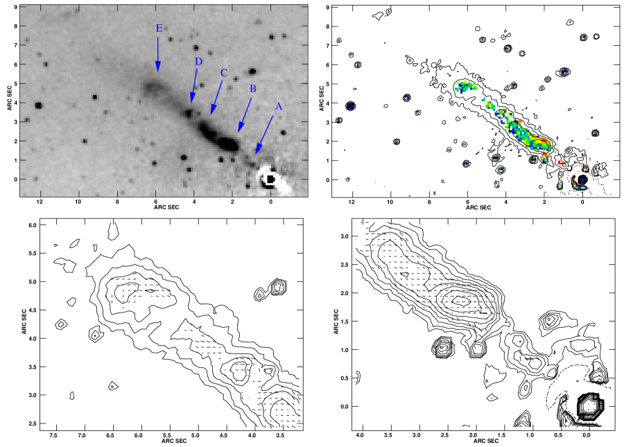
Figure 2: Optical polarimetry of the 3C 66B jet. The image scale is 440 pc/arcsec. The top left panel shows our Stokes I image with knots labelled following Hardcastle et al. (2001). At top right, we show fractional polarization (colors) overplotted with total intensity contours - red indicates $\lower 2.15277pt\hbox{$\;\buildrel>\over{\sim}\;$}30\%$ polarization. At bottom left, we show contours of total intensity superposed with polarization (apparent B field) vectors for the outer part of the jet - knots D and E -, and at bottom right we show the same for the inner part of the jet - knots A, B, and C; a vector $1^{\prime\prime}$ long represents 400% polarization; and contours are spaced by powers of 2. The presence of a nuclear dust ring (Sparks et al. 2000) can be seen in the residuals from galaxy subtraction in the top left panel. Note the stability of the direction of the magnetic field in the 3C 66B jet. See §3 for discussion.

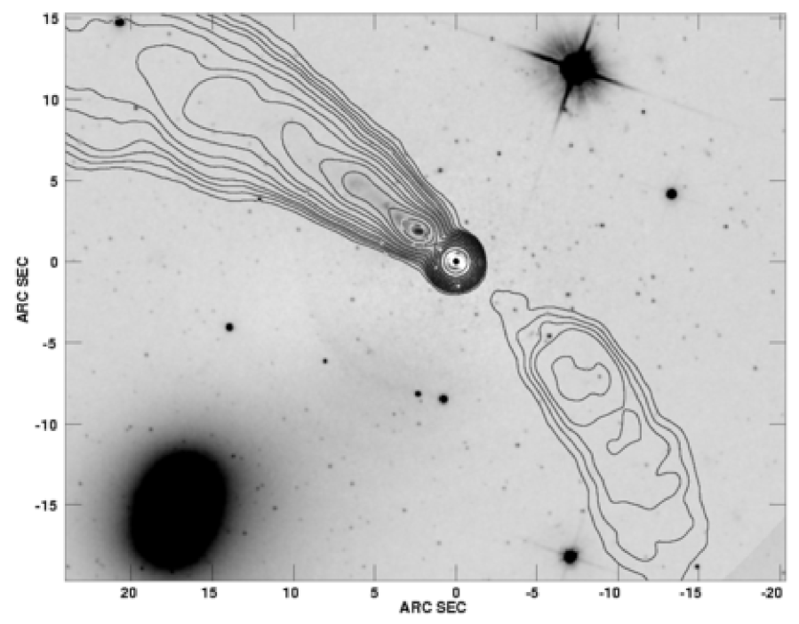
Figure 3: 3C 66B Stokes I, galaxy subtracted image overplotted with radio contours. This shows that we do not detect convincingly any counterjet emission. In particular, note the large number of point sources in the region of the counterjet, as well as over the entire field; many of these are likely globular clusters associated with the host galaxy.

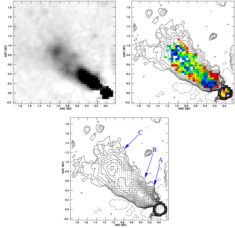
Figure 4: Optical polarimetry of the 3C 78 jet. The image scale is 600 pc/arcsec. The top left panel shows our Stokes I image. It has been scaled to bring out the faint outer parts of the jet. At top right, we show fractional polarization (colors) overlaid with contours of total flux - red indicates $\lower 2.15277pt\hbox{$\;\buildrel>\over{\sim}\;$}40\%$ polarization - , while in the bottom panel, we show contours of total intensity with polarization (apparent B field) vectors; a vector $0.1^{\prime\prime}$ long represents 100% polarization; and contours are spaced by $\sqrt{2}$. The 3C 78 jet shows a wide variation in the degree of polarization, but a relatively constant magnetic field direction, as can be seen. All three knots show reduced polarization at flux maximum. See §3 for discussion.

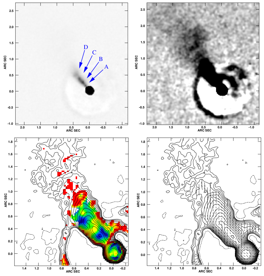
Figure 5: Optical polarimetry of the 3C 264 jet. The image scale is 440 pc/arcsec. In the upper panels, we show two views of the Stokes I image. The top left panel shows a view designed to bring out fine-scale structure within the knots, while the top right panel shows a stretch that saturates on bright regions, but helps bring out faint structure in this jet. Only in the view at top right can the jet even be seen beyond the dust ring at $1^{\prime\prime}$ from the nucleus (Sparks et al. 2000). At bottom left, we show fractional polarization (colors) overlaid with contours of total flux - red indicates $\lower 2.15277pt\hbox{$\;\buildrel>\over{\sim}\;$}45\%$, while at bottom right, we show contours of total intensity with polarization (apparent B field) vectors; a vector $0.1^{\prime\prime}$ long represents 150% polarization; and contours are spaced by $\sqrt{2}$. The 3C 264 jet shows similar characteristics to the jet of 3C 78, with wide variation in the degree of polarization but a nearly constant magnetic field direction. The low-polarization regions appear to form a “channel” down the jet centerline. See §3 for discussion.

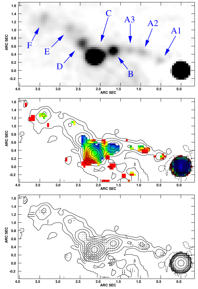
Figure 6: Optical polarimetry of the 3C 346 jet. At top, Stokes I (total intensity), at middle, fractional polarization (colors) overlaid with contours of total intensity - red indicates $\lower 2.15277pt\hbox{$\;\buildrel>\over{\sim}\;$}40\%$ polarization , and at bottom, contours of total intensity superposed with polarization (apparent B field) vectors; a vector $1^{\prime\prime}$ long represents 1000% polarization; and contours are spaced by powers of 2. The bright region to the south of the jet is a residual from galaxy subtraction, due to the presence of a nearby galaxy. In the 3C346 we do not see high polarizations in all jet components; some of the faint knots are too faint to detect in polarized light. The bright knots show significant variation in degree of polarization as well as magnetic field direction, with a strong rotation, accompanied by increased polarization at the location of the jet’s prominent bend. See §3 for discussion.

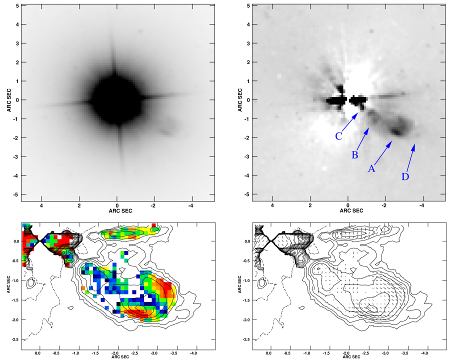
Figure 7: Optical polarimetry of the 3C 371 jet. At top left, Stokes I (total intensity) without point source or galaxy subtraction, and at top right Stokes I with our model subtracted. At bottom left, fractional polarization (colors) overlaid with contours of total flux - red indicates $\lower 2.15277pt\hbox{$\;\buildrel>\over{\sim}\;$}30\%$ polarization. At bottom right, contours of total intensity superposed with polarization (apparent B field) vectors; a vector $1^{\prime\prime}$ long represents 350% polarization; and contours are spaced by $\sqrt{2}$. The apparent negatives surrounding the nucleus are residuals from galaxy subtraction, combined with point-source mitigation techniques described in the text. Note the rich polarization structure in this jet, with large variations in both degree and direction of polarization. Perhaps most prominent is the large, low-polarization “channel” that appears to extend down the length of the brightest jet component. See §3 for discussion.

Our results are shown in Figures 1-7. Each of these shows one or more views of the Stokes I image; where necessary, we include views with both high and low contrast as well as multiple fields of view. We give two views of the polarimetry of each jet, both in fractional polarization overlaid with flux contours, and as a polarization vector image with flux contours. Each image is in a north-up, east-left configuration, and all images have been galaxy subtracted. We have clipped the polarization maps at the 3 $\sigma$ level. As can be seen, these jets display a broad variety of morphologies, both in total intensity as well as polarization. Three jets (3C 15 [Figure 1], 3C 346 [Figure 6] and 3C 371 [Figure 7]) are rather knotty, while three others (3C 66B [Figures 2, 3], 3C 78 [Figure 4], and 3C 264 [Figure 5]) are much smoother.

We give background information on these sources, as well as all other jets imaged polarimetrically with HST, in Table 2. The columns in Table 2 are, in order: (1) The source name; (2) its redshift; (3) the total power at 178 MHz (a measure of the power put out by the entire source; at this low frequency it is usually dominated by the lobes); (4) The FR type (Fanaroff & Riley 1974); (5) and (6) The length of the jet as seen in the radio and optical (in kpc); (7) The mean surface brightness (in R band); (8) References and notes; (9) Average polarization in the jet.

Table 2: Jets with HST Polarimetry

Source	$z$	$\log P_{178}$	FR	$L$(rad)	$L$(opt)	$\mu_{R,ave}$	Ref./	Avg.
		W/Hz	Type	kpc	kpc	mag/arcsec2	Notes	%P
M87	0.0044	25.6	I	89	2.0	16.3	1,2,3	35
3C 15	0.0730	26.2	I/II	66	8.4	20.4	4	20
3C 66B	0.0213	25.4	I	153	2.7	20.3	4	20
3C 78	0.0287	25.5	I	129	1.0	18.9	4	12
3C 264	0.0217	25.4	I	41	1.1	17.9	4	25
3C 273	0.1583	27.6	II	62	62	20.8	5	$\sim$10
3C 293	0.0450	25.0	I/II	210	1.5	24.1	6,7	$\sim$6
3C 346	0.1620	26.8	II	37	7.4	18.3	4	23
3C 371	0.0510	25.3	I	284	4.0	20.4	4	21

3C 15. 3C 15 (Figure 1) is a radio galaxy at a redshift $z=0.073$. At radio frequencies, it shows diffuse emission from extended radio lobes, a bright, one-sided jet as well as a weak counter-jet (Leahy et al. 1997). Its overall radio power places it at the low end of the FR II regime (i.e., $L_{178{\rm MHz}}\lower 2.15277pt\hbox{$\;\buildrel>\over{\sim}\;$}10^{25}{\rm~{}W~{}Hz^{-1}}$, Fanaroff & Riley 1974), while its edge-dimmed, diffuse morphology is more characteristic of FR I galaxies (as opposed to FR IIs where prominent hotspots are more commonly seen). Its optical jet was first discovered with HST observations (Martel et al. 1998), and X-ray observations with Chandra were discussed by Kataoka et al. (2003). At 8.4 kpc long, its optical jet is over four times longer in projected size than that of M87 (Sparks, Biretta & Macchetto 1996).

The jet emission is resolved into four knot regions on radio maps (Leahy et al. 1997), three of which can be seen in the optical (Martel et al. 1998). The HST also resolves the innermost of the radio emission regions into two fairly distinct knots. Here we follow the scheme of Martel et al. (1998) in referring to the emission regions in the 3C 15 jet, and label them A through D, respectively, outwards from the nucleus. X-ray emission is seen only from two knots (A and C; Kataoka et al. 2003, Dulwich et al. 2006). The jet’s optical polarization averages about 20%. The highest optical polarizations are seen along the outer edges (specifically away from knot maxima) of the knot A-B complex ($\approx 30\%$), as well as at the ends of knot C (35-40%). Reduced polarizations are seen in a curved region that extends throughout the A-B complex, with minima near the flux maxima of knots A and B ($\approx 0$ and $5\%$, respectively). The predominant MFPA seen in the optical in the A-B complex is parallel to the jet, but significant rotations are seen near the flux maximum of A as well as in a region inclined to the jet direction through B and at the downstream end of B. Further out, in knots C and D, the predominant MFPA we see is perpendicular to the jet. In Dulwich et al. (2006), we interpret these changes as evidence of a helical twist in the magnetic field in knots A and B, followed by a strong shock at knot C.

3C 66B. 3C 66B (Figures 2 and 3) is the nearest of our jet sources, at a redshift of $z=0.0213$ (Stull et al. 1975). Its optical counterpart is an elliptical galaxy associated with a small group in the vicinity of the cluster Abell 347. The optical galaxy features a dust disk, at a radius of $0^{\prime\prime}.5$, as was noted by Sparks et al. (2000); evidence of this feature can also be seen on our images (Figure 2). Its radio structure is a hybrid between an edge-darkened double and a head-tail morphology (Leahy, Jägers & Pooley 1986; Hardcastle et al. 1996). A two-sided inner radio jet extending over $25^{\prime\prime}$ is seen, with both jets curving towards the East at distances $>20-30^{\prime\prime}$ from the core. The optical jet emission was first detected by Butcher, van Breugel & Miley (1980), and further ground-based work (Fraix-Burnet, Nieto & Poulain 1989) revealed the presence of five distinct knots (for which we use the terminology of Hardcastle et al. 1996) of polarized optical emission, corresponding to the location of known radio knots. The first HST images of the 3C 66B jet were discussed by Macchetto et al. (1991), and the jet has also been imaged with ISO (Tansley et al. 2000) and Chandra (Hardcastle et al. 2001).

A tentative detection of the southern counter-jet was claimed in $I$ band by Fraix-Burnet (1997), based on ground-based imaging. As shown in Figure 3, while there are some objects in the region of the counter-jet corresponding to the regions claimed by Fraix-Burnet (1997), they appear more likely to be point sources (perhaps globular clusters) than extended counter-jet features. They do not exhibit any significant polarization structure at the levels that we are able to detect, and given the multitude of globular clusters in the field, this seems a more likely explanation. A more in depth analysis of the spectra of these features will be presented in an individual paper on this object, including several more bands from the HST archive.

The jet of 3C 66B rivals that of M87 (n.b., the jets of 3C 273 and 3C 403 have roughly similar angular extents, but are only bright for $\lower 2.15277pt\hbox{$\;\buildrel<\over{\sim}\;$}50\%$ of their extents) for the longest angular length optical jet feature known. It also rivals M87 for the sheer variety of structure: while the majority of the optical emission comes from a region that appears smooth at lower resolution (often referred to as knots B and C), high-resolution HST images reveal a number of rather sharp, abrupt structures on a variety of distance scales. While we see optical emission from the entire length of the jet, our HST polarimetry has high-enough signal to noise to image the polarization morphology of 3C 66B’s jet for just over $7^{\prime\prime}$.

3C 66B shows a wide variation in fractional polarization, with a minimum at the downstream end of knot B ($\sim 10\%$) and a maximum ($\sim 35\%$) at knot B’s upstream edge. Knot D displays a 90^∘ rotation in MFPA across large regions of its flux maximum, while a smaller rotation of the magnetic field is seen in the broad, flux maximum region of knot B, with the field vectors running parallel to the flux contours, at an angle of $\sim 45^{\circ}$ to the jet propagation direction. Knot E also shows a strong rotation in the MFPA, with magnetic field vectors approximately perpendicular to the jet and parallel to the local flux contours. These characteristics are classic markers of a perpendicular bow shock. Unlike several of the other jets in our sample (3C 78 and 3C 264, this paper; also M87’s knot A-B region, as in Perlman et al. 1999), in 3C 66B’s jet we do not see significant increases in fractional polarization at the edges accompanying a near-constant MFPA in the interior. Small regions of $90^{\circ}$ rotation in MFPA are seen near the polarization minima, suggesting that superposition plays a part in what we see from these regions. This combination of characteristics makes 3C 66B’s polarization morphology unique among our sample.

3C 78. The radio source 3C 78 (Figure 4) is hosted by the E/S0 galaxy NGC 1218, at a redshift of $z=0.0289$. The optical galaxy has a face-on dust disk (Sparks et al. 2000). Its radio structure (Saikia et al. 1986, Unger et al. 1984, Jones, Sramek & Terzian 1981) shows on the largest scales a two-sided source with both jets surrounded by an edge-dimmed “halo” of emission. The two jets lie at about 120^∘ from one another on kpc scales, suggesting a wide-angle tail morphology. Its 178 MHz radio power lies near the FR I/FR II boundary, as commonly seen for wide-angle tail type sources. On smaller scales, only the NE jet is seen, with bright emission extending about $2^{\prime\prime}$ from the core. The optical emission from its jet, which extends for about $1.5^{\prime\prime}$, was first discovered by Sparks et al. (1995).

The radio and optical morphology of the 3C 78 jet is remarkably smooth, with only a few bright knots. Our image shows polarized emissions averaging $\sim 12\%$ for the entire length of the optical jet. It also shows evidence of oversubtraction in the inner regions, due to difficulty in fitting out the surface brightness variations due to the dust lane. 3C 78 shows the least variation in fractional polarization of all the jets in this sample. We do, however, observe lower polarizations near the jet center, and maxima at the jet edges (reaching as high as 50%) and in interknot regions (15-25%). Only minor changes in magnetic field position angle are seen, even in knot flux maxima. The only significant changes that are seen occur in two regions: at $0.1^{\prime\prime}$ from the nucleus (just outside the area where there is significant residual from PSF subtraction) the MFPA is perpendicular to the jet direction, then switches within $0.1^{\prime\prime}$ to a parallel configuration. A more subtle feature is seen at about $0.7^{\prime\prime}$ from the nucleus (near the end of the brightest region of the jet), where the MFPA largely follows flux contours, around 30^∘ away from the jet direction.

3C 264. 3C 264 (Figure 5) is the second-nearest object discussed in this paper, at a redshift $z=0.0217$. Its host galaxy is NGC 3862, an elliptical galaxy in Abell 1367. The optical galaxy has a face-on dust ring at radii between $0.75^{\prime\prime}$ and $1^{\prime\prime}$, as noted by Sparks et al. (2000) and also seen in our data, and a relatively flat isophotal distribution inside these radii. The galaxy’s nuclear spectral energy distribution (SED) was found to be relatively similar to those of BL Lac objects, suggesting that it might house a slightly misaligned analog to those sources (Capetti et al. 2000, Rector et al. 2000). 3C 264 has a Fanaroff-Riley type I radio structure (e.g., Fanaroff & Riley 1974) with a head-tail morphology. The radio jet extends $\sim 25^{\prime\prime}$ along a direction that is initially towards the northeast, but bends towards the north at $3-6^{\prime\prime}$ from the nucleus, and then back towards the northeast at greater distances (Gavazzi, Perola & Jaffe 1981; Bridle & Vallée 1981; Baum et al. 1988; Lara et al. 1999).

The optical jet of 3C 264 was first discovered by Crane et al. (1993) in pre-COSTAR HST/FOC observations. The optically detected portion of the jet in these data is considerably shorter than the radio jet: $\sim 2^{\prime\prime}.5$ long versus $25^{\prime\prime}$, even though the Stokes I image we present here is deeper than previous optical images. Lara et al. (1997) and Baum et al. (1999) have published comparisons of the jet’s morphology in the optical and radio, as well as the first information on its optical spectral index and optical emission mechanism. The latter comparison was done on a jet-wide basis rather than for individual jet components, but importantly, Baum et al. pinned down the emission mechanism in the optical as synchrotron radiation, as seen in several other optical jets. Radio polarimetry of the 3C 264 jet has recently been discussed by Lara et al. (2004), using multi-frequency observations with the VLA and MERLIN arrays in 1997 and 1999. The jet has also recently been detected in the X-ray with Chandra (Padgett et al., in prep).

As mentioned, our Stokes I image is deeper than previous optical images of 3C 264, so we are able to describe the jet’s morphology in greater detail. The morphology is quite smooth, and even though four knots (which we label A, B, C and D in order of increasing distance from the core) are seen within the innermost arcsecond, they all represent rather small enhancements in surface brightness over the surrounding regions. Perhaps in line with its smooth appearance, the polarization morphology of this jet is very homogenous, with few changes in MFPA, and with little apparent correlation between the surface brightness and the few changes that we see. There is some trend to see lower fractional optical polarization along the jet center line and particularly at the positions of the knot maxima. By contrast, within the innermost $1^{\prime\prime}$ (the optically brightest part) the “edge” is consistently a polarization maximum. The jet undergoes a significant change in appearance and morphology when it crosses the dust lane: as previously noted by Lara et al. (1999), it fades precipitously, and then spreads out and appears to break up beyond the lane, suggesting an interaction (even though the lane appears to be seen essentially face-on, Sparks et al. 2000). Despite this, we see two enhancements in optical surface brightness in or beyond the dust lane. Because of the faintness of the jet in this region our signal to noise in $P$ is not high. However, we detect significant optical polarization beyond the dust lane ($\sim 45\%$) with MFPA aligned roughly parallel to the jet direction.

3C 346. 3C 346 (Figure 6) is the most distant object discussed in this paper, with a redshift $z=0.1610$ (e.g., Laing et al. 1983). It is a fairly compact source, and was originally classified as a Compact Steep Spectrum (CSS) object (Fanti et al. 1985). However, Spencer et al. (1991) argue that its luminous core and small, one-sided distorted jet structure are best explained by the foreshortening of a normal radio galaxy structure by a combination of a relatively small angle to the line of sight, plus beaming. In that case, its morphology and power would rank it as either a low-power FR II source or a high-power FR I. Most subsequent authors have agreed with the foreshortened FR II interpretation, and in particular Cotton et al. (1995) used the VLBI radio-core dominance and jet to counterjet ratio to argue for a viewing angle of $<32^{\circ}$ and a speed of $v=0.8c$. At low frequencies, this radio source appears double-lobed, with a kinked jet that breaks up into a number of knots at high ($>8$ GHz) frequencies (Cotton et al. 1995, van Breugel et al. 1992).

The optical host to this radio source is a 17th magnitude galaxy. It has a companion that is nearly as bright about $4^{\prime\prime}$ to the south. Optical emission from its jet was first discovered by Dey & van Breugel (1994), who found excess emission in ground-based U and R images which they attributed to the brightest two radio knots, called knots B and C by van Breugel et al. (1992). HST snapshots (de Koff et al. 1996, de Vries et al. 1997) revealed an excellent correspondence between the locations of optical and radio bright knots, with optical emission seen from all regions of the radio jet. Neither of the lobes is seen in the optical. X-ray emission from 3C 346 was first detected with Einstein (Fabbiano et al. 1984). ROSAT and ASCA observations revealed that the source’s X-ray emissions contained contributions both from a power-law, presumably nuclear jet-dominated component, plus a thermal, presumably cluster-related component. (Almudena Prieto 1996; Worrall & Hardcastle 1999, Worrall & Birkinshaw 2001). Worrall & Birkinshaw (2001) detected $\sim 3\sigma$ evidence for variability of the unresolved, power-law component. More recently, Chandra observations (Worrall & Birkinshaw 2005) show X-ray emission associated with (but offset somewhat from the flux maximum of) the radio-optical knot C.

Our optical polarization map shows a wide variation in both degree and position angle of polarization (Figure 6). Knots B and D show somewhat reduced optical polarization percentages at their optical flux maxima as compared to regions just downstream. However, knot C shows a more complex structure, with a maximum in polarization at its southeast edge, near the location of the bend, and a general gradient in polarization extending northwest to southeast. We do not have adequate signal to noise in most other knot regions. Published radio polarization maps of 3C 346 (Akujor & Garrington 1995, van Breugel et al. 1992) do not show either of these tendencies. Also, the optical polarization maps show a fairly complex morphology in MFPA. In most parts of the optical jet the magnetic field vectors track the flux contours and hence are parallel to the jet direction. However, a strong rotation of the MFPA is observed in the knot C region, agreeing with the model postulated by Worrall & Birkinshaw (2005) that attributes the bend at this location to an oblique shock, possibly associated with a wake caused by the passage of the companion galaxy. We may also observe perpendicular optical MFPA both in knot D as well as about 1” downstream, near the terminus of the main optically-bright region of the jet; however, the signal to noise is much lower in that region. .

3C 371. 3C 371 (Figure 7) is a well-known object, first associated with the BL Lac class by Miller (1975), and later included in the 1 Jy sample of BL Lacs by Stickel et al. (1991). It is among the nearest and brightest BL Lacs, with a redshift of $z=0.0510$. Its radio morphology consists of two lobes and a $25^{\prime\prime}$ long, one-sided radio jet (Wrobel & Lind 1990, Akujor et al. 1994). It has one of the highest jet to counterjet ratios known, 1700:1, implying a viewing angle $\theta<18^{\circ}$ and a bulk Lorentz factor $\Gamma\geq 3.2$ (Gomez & Marscher 2000). However, despite frequent monitoring with the VLBA, no superluminal motion has been detected, making it a bit of an oddity in the BL Lac class. Optical jet emission from 3C 371 was first detected in ground-based images by Nilsson et al. (1997), and then confirmed in HST observations by Scarpa et al. (1999). Those authors noted optical emission from three jet regions, specifically knots B ($1.7^{\prime\prime}$ from the nucleus), A ($3.1^{\prime\prime}$ from the nucleus) and D ($4.5^{\prime\prime}$ from the nucleus), and showed that in the region of overlap, the optical and radio emission tracked one another closely. X-ray emission from the jet was first discovered by Pesce et al. (2001), using Chandra observations, which detect knots A and B only.

Our Stokes I image is considerably deeper than the image published by Scarpa et al., and clearly shows emission from the region between knots B and A. From this we see that knot B appears to have a double structure, with a second maximum about $0.6^{\prime\prime}$ downstream from the main one. Emission is also seen from the inner $1.5^{\prime\prime}$ of the jet, although it is difficult to decipher its morphology due to contamination from the diffraction spikes of the nuclear point source (n.b., this issue was not discussed by Scarpa et al., although the emission is clearly shown in their images - their Fig. 3). The additional depth of our image allows us to rule out the possibility of a constant radio-to-optical spectral index $\alpha_{ro}$ (Scarpa et al. 1999); we will present more details about the spectral structure in an upcoming paper.

The polarization structure revealed by our data is complex. In the innermost region of the jet (knot C), we detect polarized emission although the signal there is somewhat affected by the diffraction spikes. In this region the polarization appears relatively constant in fraction as well as direction (approximately perpendicular to the flux contours). In knot B, we see a polarization consistent with zero at the flux maximum, with only slight rotations in the MFPA in the surrounding, moderately polarized region. The most complex structure, however, is seen in knot A and the interknot region between knots A and B. The A-B interknot region and the upstream end of knot B display perpendicular magnetic fields and moderate polarizations. Immediately downstream of this, however, near the centerline of the jet we see a virtually unpolarized channel that is about $0.4^{\prime\prime}$ wide at the upstream end of the knot and $0.2^{\prime\prime}$ wide at the downstream end. Surrounding this channel on both sides are $\sim 0.5-1^{\prime\prime}$ wide regions where the polarization increases smoothly and monotonically as one goes to the edge of the jet and the MFPA generally follows the flux contours, with a gradual rotation to a perpendicular orientation at the downstream end. Our signal to noise is not high enough to detect polarized emissions from knot D.

4 Polarization Properties of Jets

With this paper, we have increased from 3 to 9 the number of jets for which there exists optical/near-IR polarimetry with $\sim 0.1^{\prime\prime}$ resolution. Of the other three jets that have been observed polarimetrically with HST, only one (M87; see in particular Perlman et al. 1999, Capetti et al. 1997) has a signal to noise that is comparable to most of the sources described here. This is largely a byproduct of the surface brightness of the sources, as shown by Table 2, as well as the instrument configuration used. The polarimetry observations of the remaining two sources, 3C 293 and 3C 273, have significantly lower S/N. The S/N for the 3C 293 observations (Floyd et al. 2005) comes close to that attained for the faintest jet regions discussed here, thanks to the fact that NICMOS, rather than an optical instrument, was used for those observations (the knots of the 3C 293 jet have SEDs that exhibit very sharp breaks at a few microns [$R-K\approx 6$] both for intrinsic as well as extrinsic – i.e., obscuration within the host galaxy – reasons). However, in all but the brightest regions, the S/N of the 3C 273 jet observations (Thomson et al. 1993) is too low to be useful, and indeed its results are in serious conflict with much higher S/N (albeit lower resolution) ground-based polarimetry (Röser et al. 1996).

An examination of Table 2 shows that the sources with existing HST polarimetry are strongly biased towards low powers. Only three of the nine sources are nominally of the FR II class, although a fourth has been called FR II by some authors. This observational bias is largely a byproduct of having observed the optically brightest jets known in 1999, which were concentrated in relatively low-z sources. This can be seen considerably better when one looks at the total and jet radio powers at 5 GHz (data gathered from Liu & Xie 2002). We show this in Figure 8, and plot in addition to these 9 sources the seven highest optical surface brightness quasar and FR II jets (Sambruna et al. 2004, Kraft et al. 2005). Figure 8 makes apparent the fact that, even with these observations, there is still a large gap in our understanding of the magnetic field structure of jets at optical frequencies, particularly at high luminosities. Further observations (to be requested in future cycles) are needed to fill this gap.

Even with the above proviso, however, it is still useful to take stock of what we know about the polarization properties of jets in the optical. What is quite obvious from these data as well as previous observations is that jets display a great variety of optical polarization properties. Most objects seem to display at least some variation in either optical polarization percentage or magnetic field direction, although only small variations are seen in the jets of 3C 66B (Figure 2), 3C 78 (Figure 4) and 3C 264 (Figure 5). High optical polarization seems to be quite typical, averaging $\sim 20\%$ in bright regions, and reaching values as high as $50-70\%$ in a few jet regions (for example, M87, Perlman et al. 1999, 2003; some regions of the 3C 78 [Figure 4] and 3C 346 jets [Figure 6]). All but one of these very high polarization loci are well separated from their local flux maximum (the exception being knot HST-1 of the M87 jet during its recent flare, Perlman et al. 2003). However, all of them seem to be in regions where there is some other indication of a strong shock, as we discuss below for polarization maxima in general. From this, we can draw two fairly general inferences: first, that the apparent magnetic field orientation shown by these maps in optically emitting regions is well ordered, and second, that the ordering of the magnetic field is significantly affected by local, dynamical features within the jet flow. The first of these conclusions is similar to that based on radio polarization maps of jets (e.g., Bridle & Perley 1984). It is important to emphasize that what these maps show us is the ordering and direction of the magnetic field in the direction perpendicular to our line of sight. This is indicative of the overall ordering and direction of the magnetic field, although components along the line of sight are not traced by polarization data. The effect of this last point is dependent on the orientation of the jet and its various dynamical features. (Laing 1980, 1981; Hughes, Aller & Aller 1985; Cawthorne & Cobb 1990). For example, in the cases of oblique shocks (Cawthorne 2006) or anisotropic, disordered magnetic fields (Laing & Bridle 2002; Canvin & Laing 2004; Canvin et al. 2005), the combination of tangled magnetic fields with an oblique line of sight can cause the polarization vector field to be an imprecise indication of what the field directions are.

Regions of locally high polarization appear to be observed in two types of regions within optical jets. When a region of high polarization is seen close to a flux maximum and within the jet interior it is often, but not always, associated with the region upstream of that flux maximum, with much lower optical polarization being observed at the flux maximum. Several such regions are seen in the M87 jet (Perlman et al. 1999), and it is also seen in some other objects, for example knot A of the 3C 273 jet (Thomson et al. 1993), two of the knots in the 3C 15 jet (Figure 1) and knot C of the 3C 371 jet (Figure 7). As has been previously noted by Perlman et al. (1999), radio maps of most jets do not show these trends as strongly. This is consistent with shocks at these loci, where the local magnetic field is strongly compressed at the front. The shock fronts are likely to be a site of particle acceleration, as in M87 (Perlman & Wilson 2005), where enhanced X-ray emission and harder spectra are seen coincident or nearly coincident with polarization minima, suggesting that at these loci the magnetic field might be highly disordered leaving more energy available for particle acceleration. Because of the correlation with particle acceleration, the optical polarization maps will show the trend much more clearly than the radio maps, which are far less sensitive to local jet dynamics. However, a full understanding of the interaction between the magnetic fields in jets, their dynamics and the resulting multiwaveband emission will require an understanding of all scales. We will return to this subject in future papers, and we hope that these data will stimulate future theoretical work.

Locally high polarizations are also seen near the outer edges of the jet, the vectors appear to follow the local flux contours, suggesting shearing along the edge of the jet. Similar trends have been seen in radio polarization maps (e.g., Bridle & Perley 1984; Owen, Hardee & Cornwell 1989). This trend is particularly marked in apparent “working edges” in regions where bends are seen, as in, e.g., 3C 346, as well as 3C 15. In these cases, the magnetic field vectors appear to track the jet bend, indicating a strong link between the local magnetic field and the dynamical factors that are bending the jet. Regions in two other jets appear to have low polarization “channels” along the centerline of the jet, either within one very large knot complex (as in the case of the 3C 371 jet, see Figure 7) or following the ridgeline between multiple knot maxima (as in the case of the 3C 78 jet, see Figure 4). In these regions, we could have interior regions with B perpendicular to the jet, thus cancelling the polarization of the sheath (as originally suggested by Owen, Hardee & Cornwell 1989 to explain the radio polarization morphology in some regions of the M87 jet), or alternatively the magnetic field in these regions is heavily tangled, a model which makes rather less sense given the lack of strong radio flux maxima.

5 Summary

We have presented HST optical imaging polarimetry for six optical jets, thus increasing from 3 to 9 the list of objects for which data of this type exist. The objects seem to split into two classes, with three showing rather simple magnetic field structures (3C 66B, 3C 78 and 3C 264), but more complex variations seen in the remainder.

We have found a wide range of optical total flux and polarization morphologies, which correlate with one another in a wide variety of ways. We do, however, see three trends in the data. As in the radio, we find that the fractional polarization is often increased along the edges or most or all of these jets, with an MFPA that follows the jet direction. However, somewhat differently from the radio, we find that optical flux maximum regions are often (but not always) associated with local minima in fractional polarization, and that maxima in fractional polarization are usually well separated from the local flux maxima. We do not, however, find a universal or near-universal pattern. Variations in polarization are often, but not always, associated with rotations in MFPA. We see changes in MFPA in many knot regions, but not all. Thus the patterns seen in Perlman et al. (1999) are not universal to all jets, but we do see evidence that they are common to most strong, shock-like features within jets.

The picture that emerges for jets is therefore rather complex, and it is quite likely that a great many factors could contribute to the general character of a given jet’s magnetic field structure. There does appear to be a general correlation between overall “knottiness” and the complexity of polarization structure, and the most complex structures are seen in regions that are either shock-like or associated with apparent bends in the jet. Thus we can say with some certainty that the magnetic field in jets is strongly affected by local dynamics, and that this trend is seen much more prominently in optical maps. There is also a hint of a correlation between the complexity of polarized structure and jet power, suggesting some role for initial power as well as perhaps jet speed in determining the overall nature of the magnetic field structure in the jet as a whole. However, it is important to stress that at the present time this statement cannot be extended to the higher powers typical of FR II like objects due to the dearth of observations in this power range. Indeed, a full understanding of the interaction between the magnetic fields in jets, and the relevant physical parameters over the full range of jet properties, will require an understanding of the jet emission on all scales, across the electromagnetic spectrum.

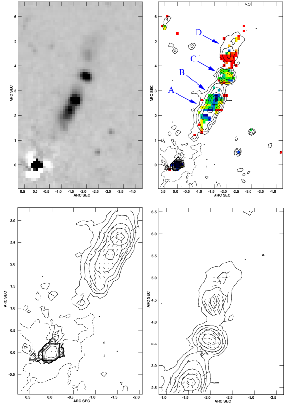
Figure 1: Optical polarimetry of the 3C 15 jet. The image scale is 1.39 kpc/arcsec. At top left, Stokes I (total intensity), and at top right, fractional polarization overlaid with contours of total intensity - red indicates $\lower 2.15277pt\hbox{$\;\buildrel>\over{\sim}\;$}45\%$ polarization. At bottom left, contours of total intensity superposed with polarization (apparent B field) vectors of the inner jet region - knots A and B - , and at bottom right, the same for the outer jet regions - knots C and D. A vector $1^{\prime\prime}$ long represents 500% polarization, and contours are spaced by powers of 2. The image has been galaxy subtracted (see §2 for details), and in all frames, north is up and east is to the left. The apparent negatives in flux surrounding the nucleus are residuals from galaxy subtraction in the innermost regions; the likely reason behind these features is nuclear dust. As can be seen, the 3C 15 jet shows rich polarization structure, with field rotations in at least three components and wide variations in the degree of polarization. See §3 for discussion.

Figure 8: The radio jet power (at 5 GHz) and total power (at 1.4 GHz) of the jets with HST polarimetry (data from Harris 2003, Jester 2003 and Liu & Zhang 2002), compared with the brightest Quasar and FR II jets (data from Sambruna et al. 2004 and Kraft et al. 2005). Note that the jets discussed in this paper are clustered mainly at relatively low power, typical of FR I sources, while in only one high-power source, 3C 273, has the jet been observed polarimetrically in the optical, and its polarization data (Thomson et al. 1993) are low S/N.

References

- (1) Akujor, C. E., Garrington, S. T., 1995, A&A Supp., 112, 235
- (2) Akujor, C. E., Luedke, E., Browne, I. W. A., Leahy, J. P., Garrington, S. T., Jackson, N., Thomasson, P., 1994, A&A Supp., 105, 247
- (3) Allen, M. G., et al., 2002, APJS, 139, 411
- (4) Almudena Prieto, M., 1996, MNRAS, 282, 421
- (5) Anderson, J., King, I., 2003, PASP, 803, 113
- (6) Anderson, J., King, I., 2004, ACS Instrument Science Report 04-15
- (7) Baum, S. A., 1997, ApJ, 483, 178
- (8) Baum, S. A., Heckman, T. M., Bridle, A., van Breugel, W. J. M., Miley, G. K., 1988, ApJS, 68, 643
- (9) Biretta, J. A., McMaster, M., 1997, WFPC2 Instrument Science Report 97-11
- (10) Boksenberg, A., et al. 1992, A & A, 261, 393
- (11) Bridle, A. H., Perley, R. A., ARAA, 22, 319
- (12) Bridle, A. H., Vallee, J. P., 1981, AJ, 86, 1165
- (13) Butcher, H. R., van Breugel, W. J. M., Miley, G. K., 1980, ApJ, 235, 749
- (14) Canvin, J. R., Laing, R. A., 2004, MNRAS, 350, 1342
- (15) Canvin, J. R., Laing, R. A., Bridle, A. H., Cotton, W. D., 2005, MNRAS, 363, 1240
- (16) Capetti, A., Macchetto, F. D., Sparks, W. B., & Biretta, J. A., 1997, A& A, 317, 637
- (17) Capetti, A., et al., 2000, ApJ, 544, 269
- (18) Cawthorne, T. V., 2006, MNRAS, 367, 851
- (19) Cawthorne, T. V., Cobb, W. K., 1990, ApJ, 350, 536
- (20) Chartas et al. 2000, ApJ, 542, 655
- (21) Chiaberge, M., et al., 2005, ApJ, 629, 100
- (22) Cotton, W. D., Feretti, L., Giovannini, G., Venturi, T., Lara, L., Marcaide, J., Wehrle, A. E., 1995, 452, 605
- (23) Crane, P., et al., 1993, ApJ, 402, 37
- (24) de Koff, S., et al., 1996, APJS, 107, 621
- (25) Dey, A., van Breugel, W. J. M., 1994, AJ, 107, 1977
- (26) de Vries, W. H., et al., 1997, ApJS, 110, 191
- (27) Dulwich, F., Worrall, D. M., Birkinshaw, M., Padgett, C. A., Perlman, E. S., Georganopoulos, M., 2006, submitted.
- (28) Fabbiano, G., Trinchieri, G., Elvis, M., Miller, L., Longair, M., 1984, ApJ, 277, 115
- (29) Fanaroff, B. L. & Riley, J. M., 1974, MNRAS, 167, 31p
- (30) Fanti, C., Fanti, R., Parma, P., Schilizzi, R. T., van Breugel, W. J. M., 1985, A&A 143, 292
- (31) Floyd, D. J. E., Perlman, E. S., Leahy, J. P., Beswick, R. J., Jackson, N. J., Sparks, W. B., Axon, D. J., O’Dea, C. P., 2005, ApJ, in press, astro-ph/0510853
- (32) Floyd, D. J. E., et al., 2006, ApJ, submitted
- (33) Fraix-Burnet, D., 1997, MNRAS, 284, 911
- (34) Fraix-Burnet, D., Nieto, J.–L., Poulain, P., 1989, A&A, 211, L1
- (35) Gavazzi, G., Perola, G. C., Jaffe, W., 1981, A&A, 103, 35
- (36) Gomez, J.–L., Marscher, A. P., 2000, ApJ, 530, 245
- (37) Gonzaga, S. et al., 2005, ACS Instrument Handbook, Version 6.0, (Baltimore: STScI)
- (38) Hardcastle, M. J., Birkinshaw, M., Worrall, D. M., 2001, MNRAS, 326, 1499
- (39) Hardcastle, M. J., Worrall, D. M., 2000, MNRAS, 314, 359
- (40) Hardcastle, M. J., Worrall, D. M., 1999, MNRAS, 309, 969
- (41) Harris, D. E., 2003, http://hea-www.harvard.edu/XJET/index.cgi
- (42) Hook, R.N., Walsh, J., Pirzkal, N., Freudling, W., 2000, ADASS IX, 216, P2-21
- (43) Hughes, P. A., Aller, H. D., Aller, M. F., 1985, ApJ, 298, 301
- (44) Jester, S., 2003, http://home.fnal.gov/ jester/optjets/
- (45) Jones, D. L., Sramek, R. A., Terzian, Y., 1982, ApJ, 261, 422
- (46) Kataoka, J., et al., 2003, A&A, 410, 833
- (47) Koekemoer, A. M., Fruchter, A. S., Hook, R., Hack, W., 2002, The 2002 HST Calibration Workshop, ed. S. Arribas, A. Koekemoer & B. Whitmore (Baltimore: STScI), 339
- (48) Kraft, R. P., Hardcastle, M. J., Worrall, D. M., Murray, S. S., 2005, ApJ, 622, 149
- (49) Kozhurina-Platais, V., Biretta, J. A., 2004, ACS Instrument Science Report 04-11
- (50) Laing, R. A., 1980, MNRAS, 193, 439
- (51) Laing, R. A., 1981, ApJ, 248, 87
- (52) Laing, R. A., Bridle, A. H., 2002, MNRAS, 336, 328
- (53) Laing, R. A., Riley, J. M., Longair, M. S., 1983, MNRAS, 204, 151
- (54) Lara, L., Feretti, L., Giovannini, G., Baum, S., Cotton, W. D., O’Dea, C. P., & Venturi, T., 1999, ApJ, 513, 197
- (55) Lara, L., Giovannini, G., Cotton, W. D., Feretti, L., Venturi, T., 2004, A&A 415, 905
- (56) Leahy, J. P., et al., 1997, MNRAS, 291, 20
- (57) Leahy, J. P., Pooley, G. G., Riley, J. M., 1986, MNRAS, 222, 753
- (58) Liu, F. K., Zhang, Y. H., 2002, A&A 381, 757
- (59) Macchetto, F., et al., 1991, ApJL, 373, L55
- (60) Madrid, J., et al., 2005, ApJS, submitted
- (61) Marshall, H. L., et al., 2005, ApJS, 156, 13
- (62) Martel, A. R., et al., 1999, ApJS, 122, 81
- (63) Martel, A. R., et al., 1988, ApJ, 496, 203
- (64) Miller, J. S., 1975, ApJL, 200, L55
- (65) Naghizadeh-Khouei, J., Clarke, D., 1993, A&A, 274, 968
- (66) Nilsson, K., Heidt, J., Pursimo, T., Silanpää, A., Takalo, L. O., Jaeger, K., 1997, ApJL, 484, L107
- (67) Owen, F. N., Hardee, P. E., & Cornwell, T. J., 1989, ApJ, 340, 698
- (68) Pavlovsky, C., et al. 2005, ACS Data Handbook, Version 4.0, (Baltimore: STScI).
- (69) Perlman, E. S.; Biretta, J. A.; Zhou, F.; Sparks, W. B.; Macchetto, F. D. 1999, AJ, 117, 2185
- (70) Perlman, E. S., Biretta, J. A., Sparks, W. B., Macchetto, F. D., Leahy & J. P. 2001, ApJ, 551, 206
- (71) Perlman, E. S., Harris, D. E., Biretta, J. A., Sparks, W. B., Macchetto, F. D. 2003, ApJ, 599, L65
- (72) Perlman, E. S., Wilson, A. S., 2005, ApJ, 627, 140
- (73) Perlmutter, S., et al., 1999, ApJ, 517, 565
- (74) Pesce, J. E., Sambruna, R. M., Tavecchio, F., Maraschi, L., Cheung, C. C., Urry, C. M., Scarpa, R., 2001, ApJL, 556, L79
- (75) Riess, A. G., et al., 2005, ApJ, 627, 579
- (76) Riess, A. G., et al., 2005, ApJ, 607, 665
- (77) Sambruna, R. M., Urry, M. C., Tavecchio, F., Maraschi, L., Scarpa, R., Chartas, G. & Muxlow, T. 2001, ApJ, 549, L161
- (78) Sambruna, R. M., Gambill, J. K., Maraschi, L., Tavecchio, F., Cerutti, R., Cheung, C. C., Urry, M. C., Chartas, G. 2004, ApJ, 608, 698
- (79) Scarpa, R., Urry, C. M., Falomo, R., Treves, A., 1999, ApJ, 526, 643
- (80) Schwartz, D. A., et al. 2000, ApJ, 540, L69
- (81) Serkowski, K., 1962, Advances in Astronomy and Astrophysics, Academic Press 1, 289
- (82) Sparks, W. B., Baum, S. A., Biretta, J. A., Macchetto, F. D., Martel, A. R., 2000, ApJ, 542, 667
- (83) Sparks, W. B., Biretta, J., & Macchetto, F., 1996, ApJ 473, 254
- (84) Sparks, W. B., et al., ApJL, 450, L55
- (85) Spencer, R. E., et al., 1991, MNRAS, 250, 225
- (86) Stickel, M., Fried, J. W., Kühr, H., Padovani, P., Urry, C. M., 1991, ApJ, 374, 431
- (87) Stull, M. A., Price, K. M., Daddario, L. R., Wernecke, S. J., Graf, W., Grebenkemper, C. J., 1975, AJ, 80, 559
- (88) Tansley, D., Birkinshaw, M., Hardcastle, M. J., Worrall, D. M., 2000, MNRAS, 317, 623
- (89) Thomson, R. C., Robinson, D. R. T., Tanvir, N. R., MacKay, C. D., & Boksenberg, A., 1995, MNRAS 275, 921
- (90) Thomson, R. C., Mackay, C. D., Wright, A. E., 1993, Nature, 365, 133
- (91) van Breugel, W. J. M., Fanti, C., Fanti, R., Stanghellini, C., Schilizzi, R. T., Spencer, R. E., 1992, A&A 256, 56
- (92) Wardle, J. F. C., Kronberg, P. P., 1974, ApJ, 194, 249
- (93) Worrall, D. M., Birkinshaw, M., 2005, MNRAS, 360, 926
- (94) Worrall, D. M., Birkinshaw, M., 2001, ApJ, 551, 178
- (95) Wrobel, J. M., Lind, K. R., 1990, ApJ, 348, 135
- (96)