Formation of Primordial Stars in a $\Lambda$CDM Universe

Abstract

Primordial stars are formed from a chemically pristine gas consisting of hydrogen and helium. They are believed to have been born at some early epoch in the history of the Universe and to have enriched the interstellar medium with synthesized heavy elements before the emergence of ordinary stellar populations. We study the formation of the first generation of stars in the standard cold dark matter model. We follow the gravitational collapse and thermal evolution of primordial gas clouds within early cosmic structures using very high-resolution, cosmological hydrodynamic simulations. Our simulation achieves a dynamic range of $\sim 10^{10}$ in length scale. With accurate treatment of atomic and molecular physics, it allows us to study the chemo-thermal evolution of primordial gas clouds to densities up to $\rho\sim 2\times 10^{-8}{\rm g}\;{\rm cm}^{-3}(n_{\rm H}\sim 10^{16}{\rm cm}^{-3})$ without assuming any a priori equation of state; a six orders of magnitudes improvement over previous three-dimensional calculations. We implement an extensive chemistry network for hydrogen, helium and deuterium. All the relevant atomic and molecular cooling and heating processes, including cooling by collision-induced continuum emission, are implemented. For calculating optically thick H₂ cooling at high densities, we use the Sobolev method (Sobolev 1960) and evaluate the molecular line opacities for a few hundred lines. We validate the accuracy of the method by performing a spherical collapse test and comparing the results with those of accurate one-dimensional calculations that treat the line radiative transfer problem in a fully self-consistent manner.

We then perform a cosmological simulation adopting the standard $\Lambda$CDM model. Dense gas clumps are formed at the centers of low mass ($\sim 10^{5-6}M_{\odot}$) dark matter halos at redshifts $z\sim 20$, and they collapse gravitationally when the cloud mass exceeds a few hundred solar masses. To examine possible gas fragmentation owing to thermal instability, we compute explicitly the growth rate of isobaric perturbations. We show that the cloud core does not fragment in either the low-density ($n_{\rm H}\sim 10^{10}{\rm cm}^{-3}$) or high-density $(\sim 10^{15}{\rm cm}^{-3}$) regimes, where gas cooling rate is increased owing to three-body molecule formation and collision-induced emission, respectively. The cloud core becomes marginally unstable against chemo-thermal instability in the low-density regime. However, since the core is already compact at that point and correspondingly the sound-crossing time as well as the free-fall time are short, or comparable to the perturbation growth timescale, it does not fragment. Run-away cooling simply leads to fast condensation of the core to form a single proto-stellar seed. We also show that the core remains stable against gravitational deformation and fragmentation throughout the evolution. We trace in Lagrangian space the gas elements that end up at the center of the cloud, and study the evolution of the specific angular momentum. We show that, during the final dynamical collapse, small angular momentum material collapses faster than the rest of the gas and selectively sinks inwards. Consequently, the central regions have little specific angular momentum, and rotation does not halt collapse. With the large physical dynamic range of our simulation, we, for the first time, obtain an accurate gas mass accretion rate within a 10$M_{\odot}$ innermost region around the protostar. The protostar is accreting the surrounding hot ($T\sim 2000$K) gas at a rate of $\dot{M}>10^{-2}-10^{-3}M_{\odot}/{\rm yr}$. From these findings we conclude that primordial stars formed in early cosmological halos are massive. We carry out proto-stellar evolution calculations using the obtained accretion rate. The resulting mass of the first star when it reaches the zero-age main sequece is $M_{\rm ZAMS}\sim 100M_{\odot}$, and less ($\gtrsim 60M_{\odot}$) for substantially reduced accretion rates.

1. Introduction

The current standard theory of cosmic structure formation posits that the present-day clumpy appearance of the Universe developed through gravitational amplification of matter density fluctuations generated in its very early history. The energy content of the Universe and the basic statistics of the initial density field have been determined with great accuracy from recent observations of the cosmic microwave background (Spergel et al. 2006), large-scale structure (Tegmark et al. 2004; Cole et al. 2005), and distant supernovae (Riess et al. 2004; Astier et al. 2006). It has become possible to make accurate predictions for the formation and nonlinear growth of large-scale structure within this framework.

The standard model based on cold dark matter (CDM) predicts that the mass variance after the epoch of matter-radiation equality has progressively larger amplitudes on smaller mass scales, indicating that objects form hierarchically, with smaller ones originating first. Although the fluctuation amplitudes on scales much smaller than galactic scales are not known directly from observations, most of the viable candidates for the dark matter predict nearly scale-invariant fluctuations down to stellar or even planetary masses. Such CDM models generically argue that the first cosmological objects are formed in low mass ($\sim 10^{6}M_{\odot}$) dark halos at high redshifts ($z\gtrsim 20$) when primordial gas condenses via molecular hydrogen cooling (Couchman & Rees 1986; Haiman, Thoul & Loeb 1996; Tegmark et al. 1997; Abel, Bryan & Norman 2002; Yoshida et al. 2003; see Bromm & Larson 2004 for a review). Hierarchical structure formation eventually leads to the emergence of a population of early generation stars/galaxies which terminate the Cosmic Dark Ages by emitting the first light (Madau 2000; Cen 2003; Miralda-Escudé 2003; Sokasian et al. 2003, 2004; Reed et al. 2005).

The first stars are also believed to be the first source of heavy element production (those heavier than lithium). Heavy elements must have been processed in massive stars and expelled into the interstellar medium by supernovae, to enable the formation of ordinary stellar populations. Early metal-enrichment of the low density intergalactic medium is also suggested by observations of the Lyman-$\alpha$ forest (Songaila 2001, 2005; Schaye et al. 2003). Interestingly, the recent discovery of extremely metal-poor stars (Christlieb et al. 2002; Frebel et al. 2005) suggests that relics from very early generation stars exist even today in our own Galaxy. Stars with such low metallicities provide valuable information on the first stars that likely polluted the interstellar medium (Iwamoto et al. 2005; Tumlinson 2006).

The study of primordial star formation has a long history. The formation of the first cosmological objects via gas condensation by molecular hydrogen cooling has been studied for many years (e.g. Saslaw & Zipoy 1967; Peebles & Dicke 1968; Matsuda, Sato, & Takeda 1969; Kashlinsky & Rees 1983). In the context of star formation, the evolution of a collapsing primordial gas cloud has also been studied extensively (Matsuda, Sato, & Takeda 1969; Yoneyama 1972; Carlberg 1981). Palla, Salpeter & Stahler (1983) used a one-zone model to follow gas collapse to very high densities. They identified a minimum Jeans mass scale of 0.1 solar mass from the thermal evolution of the cloud core, suggesting the formation of low-mass primordial stars. One-dimensional hydrodynamic simulations of spherical gas collapse were performed by a number of researchers (Villere & Bodenheimer 1987; Omukai & Nishi 1998; Ripamonti et al. 2002). Omukai & Nishi (1998) included a detailed treatment of all the relevant chemistry and radiative processes and thus were able to provide accurate results on the thermal evolution of a collapsing primordial gas cloud up to stellar densities. These authors found that, while the evolution of a spherical primordial gas cloud proceeds in a roughly self-similar manner, there are a number of differences in the thermal evolution from that of present-day, metal- and dust-enriched gas clouds.

Recently, three-dimensional hydrodynamic calculations were performed by several groups. Abel et al. (2000; 2002) and Bromm et al. (1999; 2002) studied the formation and fragmentation of primordial gas clouds in CDM models. From various analyses of the simulation results, these authors conclude that primordial stars (often called “Population III”) that form in dark matter matter halos are rather massive. Yoshida et al. (2003) examined the statistical properties of primordial star-forming clouds from a large sample of early mini-halos located in their cosmological simulations. The chemo-thermal evolution of the primordial gas clouds is rather complex, being coupled with the dynamical evolution of the assembly of dark matter halos (Yoshida et al. 2003; Gao et al. 2005), and simple analytic models based on crude assumptions almost always fail in predicting the evolution of primordial gas in CDM halos.

The three-dimensional calculations of Abel et al. (2002; hereafter, ABN02) were able to follow the gas evolution until a small ($\sim 1M_{\odot}$) fully molecular core formed. However, since they did not include the effect of the opacity of the cloud core, the radiative cooling rate is over-estimated at the cloud center. Thus their results for late stage evolution, including the important problem of fragmentation and mass accretion, are uncertain. Bromm & Loeb (2004) made similar approximations and also continued their simulation by creating a sink particle to study the late time accretion phase. None of these simulations reproduce the correct density, temperature, and velocity profiles in the vicinity the protostar, which are among the most important quantities for proto-stellar evolution. A critical technique we describe in the present paper is computation of molecular line opacities. With the implementation of optically thick line cooling, the gas evolution can be followed to much higher densities than in the previous studies. In principle, evaluating the net line cooling rate at such high densities involves costly line radiative transfer. We circumvent this by using a local Sobolev method which employs local velocity information as well as knowledge of the density and temperature. We show that the method works well in problems of collapsing gas clouds, in terms of computation of radiative cooling rates and resulting density and temperature structure. We apply this technique to cosmological simulations.

An important, outstanding issue is to determine whether or not a gas cloud fragments into multiple objects during its collapse. If it does fragment, it could yield multiple stars, suggesting the possibility of star-cluster formation including low-mass stars (Sabano & Yoshii 1977; Silk 1983). To the contrary, if the gas cloud remains stable against fragmentation throughout its evolution, it will lead to the formation of a single proto-stellar seed, surrounded by a large amount of infalling gas - a typical condition for a proposed scenario of the formation of massive stars (Larson & Starrfield 1971; see the review by Larson 2003). We show that the gas cloud formed at the center of a high-redshift halo remains stable against fragmentation, to form a single proto-stellar seed. We also find that the rate of gas accretion is very high. The mass accretion rate onto a protostar largely affects the final stellar mass (Omukai & Palla 2001; 2003). Stahler, Palla, & Salpeter (1986a,b) suggested that large accretion rates ($>10^{-3}M_{\odot}\;{\rm yr}^{-1}$) are expected for primordial protostars because of high gas temperatures in the infalling surrounding gas. For a better evaluation of the mass accretion rate, Omukai & Nishi (1998) use a self-similar solution to derive a time-dependent rate, while Tan & McKee (2004) consider effects of rotation in accretion dynamics around proto-stellar disks. We address this issue using fully self-consistent cosmological simulations. Finally, we carry out proto-stellar evolution calculations and determine the resulting stellar mass on the assumption that the true gas mass accretion rate and its time-dependence is close to the instantaneous accretion rate at the protostar formation epoch.

The rest of the paper is organized as follows. In Section 2, we describe the chemistry network used for our simulations. The relevant cooling and heating processes are described in Section 3. There, we also provide details of numerical implementation. In Section 4, we present the results of a test problem of a spherically collapsing gas. We compare our results to previous work using one-dimensional codes. We present the results of our $\Lambda$CDM cosmological simulations in Section 5. Implications of the main conclusions are discussed in Section 6.

2. Primordial gas chemistry

The reaction network for hydrogen and helium (e^-, H, H⁺, He, He⁺, He⁺⁺, H₂, H${}_{2}^{+}$, H^-) is largely based on that of Abel et al. (1997) and Galli & Palla (1998; hereafter, GP98). The rate coefficients are summarized in Table 1. In this section, we describe updates in detail.

2.1. Molecule formation

In a low density primordial gas, the main formation path for hydrogen molecules is via the H^- channel:

$${\rm H}+{\rm e}\rightarrow{\rm H}^{-}+h\nu\;\;\;\;\;\;({\rm reaction\;\;7}),$$ (1)

$${\rm H}+{\rm H}^{-}\rightarrow{\rm H}_{2}+e\;\;\;\;\;\;({\rm reaction\;\;8}),$$ (2)

where electrons are used as catalysts. H₂ formation via the H${}_{2}^{+}$ channel (reaction 9, 10) is dominant at very high redshifts $z>200$ where cosmic microwave background photons destroy H^- by photo-detachment (see also a recent calculation of Hirata & Padmanabhan 2006, which shows the importance of reactions involving HeH$+$ ions in H₂ production at such high redshifts.) There is considerable variation among published experimental data and theoretical calculations for the reaction rate $k_{8}$. However, uncertainty in this rate will have little effect on the H₂ abundance, because the reaction is always much faster than the formation of H^-. We use the fit by GP98 to the calculations of Launay et al. (1991) for $k_{8}$. The rate coefficients for mutual neutralization

$${\rm H}^{-}+{\rm H}^{+}\rightarrow{\rm H}_{2}\;\;\;\;\;\;({\rm reaction\;\;18}),$$ (3)

are also uncertain, particularly at low temperatures (Glover et al. 2006). This reaction affects the H₂ abundance significantly only when the ionization fraction is greater than $\sim 0.01$ (Palla & Zinnecker 1987). In the calculations presented below, the ionization fraction is always smaller than $10^{-3}$, and hence the uncertainty in the reaction rate is unimportant. We use the fit given in GP98. We note that a better determination of this rate is clearly needed for calculations of, for example, the evolution of cooling gas in relic Hii regions (Oh & Haiman 2002; Glover et al. 2006; Yoshida 2006; Susa & Umemura 2006).

2.2. Three-body reactions

At high densities ($n_{\rm H}>10^{8}{\rm cm}^{-3}$), hydrogen molecules are formed by the following rapid reactions

$${\rm H}+{\rm H}+{\rm H}\rightarrow{\rm H}_{2}+{\rm H}\;\;\;\;\;\;({\rm reaction\;\;22}),$$ (4)

and

$${\rm H}+{\rm H}+{\rm H}_{2}\rightarrow 2{\rm H}_{2}\;\;\;\;\;\;\;\;({\rm reaction\;\;23}).$$ (5)

We use the reaction coefficients as given in Palla, Salpeter, & Stahler (1983):

$$k_{22}=5.5\times 10^{-29}\;T^{-1}\;\;{\rm cm}^{6}s^{-1},$$ (6)

and

$$k_{23}=6.875\times 10^{-30}\;T^{-1}\;\;{\rm cm}^{6}s^{-1}.$$ (7)

Note that the net formation rate scales with the cube of density. The three-body reactions are very efficient in converting hydrogen atoms to molecules at densities $n>10^{8}{\rm cm}^{-3}$.

Krstic, Janev & Shultz (2003) recently revised reaction rates for three-body reactions involving protons,

$${\rm H}+{\rm H}+{\rm H}^{+}\rightarrow{\rm H}_{2}+{\rm H}^{+},$$ (8)

$${\rm H}+{\rm H}+{\rm H}^{+}\rightarrow{\rm H}_{2}^{+}+{\rm H},$$ (9)

and found the rates are as large as those for reactions (22), (23). Since the ionization fraction is extremely small in the primordial gas at high densities and low temperatures ($T<3000$ K), which is the range of our interest, these reactions are unimportant in the calculations presented in what follows. We note, however, that when the ionization fraction (hence proton abundance) is large in the proto-stellar gas cloud in the final adiabatic phase, or under strong ultra-violet radiation, inclusion of the reactions could be important.

2.3. Collisional dissociation of H₂

In a neutral primordial gas, H₂ molecules are destroyed mostly by collisions with H atoms and H₂ molecules:

$${\rm H}_{2}+{\rm H}\rightarrow 3{\rm H}\;\;\;\;\;\;\;\;({\rm reaction\;\;11}),$$ (10)

$${\rm H}_{2}+{\rm H}_{2}\rightarrow{\rm H}+{\rm H}+{\rm H}_{2}\;\;\;\;\;\;\;\;({\rm reaction\;\;25})$$ (11)

We use the collision cross-sections of Martin et al. (1996) for reaction 11 that include dissociation from excited levels at high densities. For dissociation by collisions with H₂ (reaction 25), we use the high density limit of Palla et al. (1983)

$$k_{25}=8.125\times 10^{-8}\;T^{-1/2}\exp\left(-\frac{52000}{T}\right)\times\left[1.0-\exp\left(-\frac{6000}{T}\right)\right].$$ (12)

Dissociation by collisions with helium atoms

$${\rm H}_{2}+{\rm He}\rightarrow{\rm H}+{\rm H}+{\rm He}$$ (13)

and its reverse reaction (three-body reaction involving helium) have much smaller reaction rates than those involving collisions with hydrogen (Dove et al. 1987), and thus we ignore these processes.

We include the charge exchange reaction between H and He (reaction 14, 15, see Glover & Brand 2003) and update the reaction rate for ${\rm H}+{\rm H}_{2}^{+}\rightarrow{\rm H}^{+}+{\rm H}_{2}$ (reaction 12) with the new fit given by Savin et al. (2004a,b). These processes become important in calculations of, for example, the evolution of relic Hii regions (Yoshida 2006), but do not affect the calculations in the present paper.

2.4. The adiabatic index

We write the equation of state for a gas consisting of atoms and molecules as

$$P=\frac{k_{\rm B}T}{\mu m_{\rm p}}\rho=(\gamma-1)\rho u,$$ (14)

where the adiabatic index is computed from

$$\gamma-1=\frac{1}{\mu}\left(\sum_{i}\frac{1}{(\gamma_{i}-1)}\right)^{-1}.$$ (15)

The summation is taken over all chemical species including helium. For the adiabatic exponent for H₂ , we use the formula in Landau & Lifshitz (1984),

$$\frac{1}{\gamma_{\rm H_{2}}-1}=\frac{1}{2}\left[5+2x^{2}\frac{e^{x}}{(e^{x}-1)^{2}}\right],$$ (16)

where the last term with $x=6100{\rm K}/T$ accounts for vibrational degrees of freedom of hydrogen molecules. At very high pressures ($P\gg 10^{4}{\rm dyne}\;{\rm cm}^{-2}$), various non-ideal gas effects become important and the equation of state needs to be modified (Saumon, Chabrier, & van Horn 1995; Ripamonti et al. 2002), but this is outside the range of gas phases we consider here.

3. Cooling and heating rates

Radiative cooling processes owing to excitation, ionization, and recombination of hydrogen and helium atoms are well established. We refer the readers to Cen (1992) , Fukugita & Kawasaki (1994), and Abel et al. (1997). We note that these cooling processes are generally unimportant in studies of the evolution of a neutral primordial gas. Below we describe more relevant molecular cooling and chemical heating processes in detail.

3.1. Cooling by H₂ and HD molecules

We use the cooling rate of Galli & Palla (1998) for H₂ line cooling in the low density limit:

$$\Lambda_{\rm H_{2}}(n\rightarrow 0)={\rm dex}[-103.0+97.59\log T-48.05(\log T)^{2}+10.80(\log T)^{3}-0.9032(\log T)^{4}].$$ (17)

At high densities, formation of H₂ molecules takes place and molecular fraction increases rapidly, making H₂ line cooling a dominant cooling process. At high densities, all energy levels are populated according to local thermodynamic equilibrium (LTE). An accurate fit for the optically thin cooling rate is given by Hollenbach & McKee (1979):

$$\Lambda_{\rm LTE}=\Lambda_{\rm rot}+\Lambda_{\rm vib},$$ (18)

where

$$\Lambda_{\rm rot}=\frac{9.5\times 10^{-22}\;T_{3}^{3.76}}{1+0.12\;T_{3}^{2.1}}\exp\left[-\left(\frac{0.13}{T_{3}}\right)^{3}\right]+3\times 10^{-24}\exp\left[-\left(\frac{0.51}{T_{3}}\right)\right],$$ (19)

and

$$\Lambda_{\rm vib}=6.7\times 10^{-19}\exp\left[-\left(\frac{5.86}{T_{3}}\right)\right]+1.6\times 10^{-18}\exp\left[-\left(\frac{11.7}{T_{3}}\right)\right],\;\;\;T_{3}=\frac{T}{1000{\rm K}}\,.$$ (20)

The low density limit and the high density limit are bridged as

$$\Lambda_{\rm H_{2}}=\frac{\Lambda_{\rm H_{2}}({\rm LTE})}{1+n_{\rm cr}/n_{\rm H}}\,,$$ (21)

where

$$\frac{n_{\rm cr}}{n_{\rm H}}=\frac{\Lambda_{\rm H_{2}}({\rm LTE})}{\Lambda_{\rm H_{2}}(n\rightarrow 0)}\,.$$ (22)

For HD cooling, we use the formulation of Flower et al. (2000) . We show the cooling rates in Fig. 3.1. There, we assume a fractional abundance of [HD/H₂] = $10^{-3}$. Cooling by HD molecules is important only at low temperatures ($T<200{\rm K}$) and low densities ($n_{\rm H}<10^{8}$); otherwise H₂ cooling dominates. We have carried out a spherical collapse simulation (see Section 4) with full deuterium chemistry for five species (D, D⁺, D^-, HD, HD⁺), using the extensive reaction network of Nakamura & Umemura (2002). We find that the fractional ratio of [HD/H₂] has a maximum of $\sim 10^{-3}$ at $n_{\rm H}\sim 10^{4}\;{\rm cm}^{-3}$, where the gas temperature is about 200 K (see Fig. 4 and also Omukai et al. 2005). Therefore, HD cooling is unimportant for the thermal evolution of initially neutral primordial gas clouds. The role of HD cooling in partially ionized gas will be studied elsewhere (Yoshida et al. 2006, in preparation).

Figure 1.— Radiative cooling rates per molecule as a function of temperature. We show the low-density limit for H₂ (solid line) and HD (dot-dashed line) assuming $n_{\rm H}=1\;{\rm cm}^{-3}$ and the relative abundance HD/H₂ = 0.001. The dashed line is the high-density limit of the H₂ cooling function.

3.2. Chemical cooling and heating

We include the heat gain associated with the formation of hydrogen molecules via three-body reactions as

$$\Gamma_{\rm H2,3b}=\epsilon_{{\rm H}_{2}}\frac{{\rm d}n_{{\rm H}_{2}}}{{\rm d}t}\,,$$ (23)

where $\epsilon_{{\rm H}_{2}}=4.48{\rm eV}$ is the molecular binding energy. We also account for heat loss owing to collisional dissociation (Section 2.3) in the same manner. The two-body formation process of H₂ molecules, either via H^- (reaction 8) or H${}_{2}^{+}$ (reaction 10), is exothermic, but deposits its energy into H₂ through rotational and vibrational excitation. These reactions can be important sources of heat at high densities where collisional de-excitation removes the excitation energy. Following Hollenbach & McKee (1979) and Shapiro & Kang (1987), we calculate the heating rates as

$$\Gamma({\rm H}^{-})=k_{8}n_{{\rm H}^{-}}n_{\rm H}[3.53(1+n_{\rm cr}/n_{\rm H})^{-1}]\;\;{\rm eV}{\rm cm}^{-3}{\rm s}^{-1},$$ (24)

$$\Gamma({\rm H}_{2}^{+})=k_{10}n_{{\rm H}_{2}^{+}}n_{\rm H}[1.83(1+n_{\rm cr}/n_{\rm H})^{-1}]\;\;{\rm eV}{\rm cm}^{-3}{\rm s}^{-1},$$ (25)

where the critical density is given by

$$n_{\rm cr}=10^{6}T^{-1/2}\left[1.6y_{\rm H}\exp[-(400/T)^{2}]+1.4\;y_{{\rm H}_{2}}\exp\left(-\frac{12000}{T+1200}\right)\right]^{-1}{\rm cm}^{-3},$$ (26)

and $y_{\rm H}$ and $y_{{\rm H}_{2}}$ are the number fractions of hydrogen atoms and hydrogen molecules, respectively.

3.3. Optically thick H₂ line cooling

When the gas density and the molecular fraction are high, the cloud becomes opaque to molecular lines and then H₂ line cooling becomes inefficient. The net cooling rate can be expressed as

$$\Lambda_{{\rm H}_{2},{\rm thick}}=\sum_{u,l}h\nu_{ul}\;\beta_{{\rm esc},ul}\;A_{ul}\;n_{u}\,,$$ (27)

where $n_{u}$ is the population density of hydrogen molecules in the upper energy level $u$, $A_{ul}$ is the Einstein coefficient for spontaneous transition, $\beta_{{\rm esc},ul}$ is the probability for an emitted line photon to escape without absorption, and $h\nu_{ul}=\Delta E_{ul}$ is the energy difference between the two levels. In the relevant temperature range $T\sim 1000-2000$K, we consider rotational levels from $J=0$ to 20, and vibrational levels $v=0,1,2$. We use the radiative transition rates $A_{ul}$ for these levels from Turner, Kirby-Docken, Dalgarno (1977). We calculate the vibrational energies $E(v,J)$ following Borysow, Frommhold & Moraldi (1989). Note that, although the net cooling rate can be directly obtained from equation (27), we use it to evaluate the reduction factor $f_{\rm red}=\Lambda_{\rm thick}/\Lambda_{\rm thin}$. For computational efficiency, we compute the cooling rate as a function of temperature using equations (18)-(20), and multiply the rate by $f_{\rm red}$ when $n_{\rm H}>10^{9}{\rm cm}^{-3}$.

In order to calculate the escape probability, we first evaluate the opacity for each molecular line as follows. The absorption coefficient for a transition from $l$-level to $u$-level is

$$\alpha_{lu}=\frac{\Delta E_{lu}}{4\pi}\;n_{l}B_{lu}\left[1-\exp\left(\frac{-\Delta E_{lu}}{kT}\right)\right]\phi(\nu)\,,$$ (28)

where $n_{l}$ is the number density of hydrogen molecules in level $l$, $B_{lu}$ is Einstein’s B-coefficient, and $\phi(\nu)$ is the line profile. We approximate the line profile by a Gaussian function

$$\phi(\nu)=\frac{1}{\sqrt{\pi}\Delta\nu_{D}}\exp\left[-\frac{(\nu-\nu_{0})^{2}}{\Delta\nu_{\rm D}^{2}}\right],$$ (29)

with the thermal Doppler width $\Delta\nu_{D}=(\nu_{0}/c)/\sqrt{kT/m_{\rm H}}$. We then compute the opacity at the line center as

$$\tau_{lu}=\alpha_{lu}L,$$ (30)

where $L$ is the characteristic length scale, which is approximately the cloud core size. Since the absorption coefficients are computed in a straightforward manner, although somewhat costly, the remaining key task is the evaluation of the length scale $L$.

It is important to recall that calculation of the photon escape probability is essentially a line transfer problem, for which, in principle, demanding radiative transfer calculations are needed to obtain accurate results. However, by noting that the important quantity we need is the effective gas cooling rate, we can formulate a reasonable and well-motivated approximation. To this end, we decided to use the escape probability method that is widely used in the study of stellar winds and planetary nebulae (Castor 1970; Goldreich & Kwan 1974). Consider a photon traveling in a gas in one direction along which a constant velocity gradient exists. The escape of photons is greatly enhanced by the presence of macroscopic velocity fields, i.e. large velocity gradients; when an emitted photon has traveled one Sobolev length to the point where the profile is Doppler-shifted by one characteristic width (line width), it can travel unimpeded and will escape from the local neighborhood.

We calculate the Sobolev length along a line-of-sight as

$$L_{r}=\frac{\;v_{\rm thermal}\;}{|dV_{r}/dr|},$$ (31)

where $v_{\rm thermal}=\sqrt{kT/m_{\rm H}}$ is the thermal velocity of H₂ molecules, and $V_{r}$ is the fluid velocity in the direction. A suitable angle-average must be computed in order to obtain the net escape probability. For a spherical cloud, the escape probability is given by

$$\beta_{\rm esc}=\frac{1-\exp(-\tau)}{\tau}\,,$$ (32)

with $\tau=\alpha L_{r}$ (Castor 1970; de Jong, Dalgarno & Chu 1975). In three-dimensional calculations, in which we do not know the exact geometry and alignment of an object, we compute the Sobolev length and the escape probability in three arbitrary orthogonal directions and take the mean as

$$\beta=\frac{\beta_{x}+\beta_{y}+\beta_{z}}{3}\,.$$ (33)

We first test the implementation in this section, and the overall accuracy of the method is examined in Section 4. Consider a homologous contracting sphere with size $R=0.01$ pc. The velocity at radius $r$ is given by

$$v(r)=rV/R\,,$$ (34)

where $V=10$ km/sec is the radial (inward) velocity at R. We set the gas temperature to be a constant at $T=1000$K and assume the gas is fully molecular with $n_{\rm H2}=5.0\times 10^{10}{\rm cm}^{-3}$. In this case, the optical depth for an emitted photon (owing to a level transition $u\rightarrow l$) is a constant

$$\tau_{lu}=\frac{\Delta E_{lu}}{4\pi}\;n_{l}B_{lu}\left[1-\exp\left(\frac{-\Delta E_{lu}}{kT}\right)\right]\frac{R}{V},$$ (35)

and the escape probability is

$$\beta_{{\rm esc},lu}=\frac{1-\exp(-\tau_{lu})}{\tau_{lu}}.$$ (36)

We run a three-dimensional simulation with the above set-up using a half million gas particles and compute the escape probability (equation [33]) at random points in the simulation region. For illustrative purpose, we consider only the rotational transition $J=6\rightarrow 4(v=0)$, which is one of the strongest lines at $T\sim 1000$K. Putting all the numerical values into equation (35), we find $\tau_{46}=3.61$ and $\beta_{46}=0.269$. From the test simulation, we obtained a mean value of $\bar{\beta}=0.2692$ within $r<0.75R$ and a maximum deviation of less than 3 %. We did not include the outer parts of the sphere ($r>0.75R$), where the density estimate is affected by the boundary. These results are quite satisfactory, and assure us that the numerical implementation is done correctly. We discuss the overall accuracy of this method in Section 4 where we perform a gas collapse simulation with density and temperature gradients. We emphasize that simple local estimates, for example, using only local densities and temperatures, do not provide correct values for the optically-thick line cooling rate, because the escape probability of line photons is greatly affected by local velocity gradients which are highly variable in both space and time.

The Sobolev method can also be extended to calculation of the self-shielding factor against photo-dissociation by Lyman-Werner photons. The feedback effects of far ultra-violet radiation is often modeled either by assuming the gas is optically thin to the photo-dissociating photons (Machacek, Bryan & Abel 2001; Ricotti et al. 2002), or by employing the formula of Draine & Bertoldi (1996) in cases with simple geometry (Omukai 2001). While accurate results can be obtained by solving radiative transfer for a number of lines, as done by, e.g., Glover & Brand (2001) in one-dimension, it will be useful to devise an approximation. The first such attempts of accounting for self-shielding have been already made, although in a much simplified manner, by Yoshida et al. (2003) and Glover et al. (2006). Our method (or its simple extension) may provide better solutions than these previous works.

3.4. Cooling by collision-induced emission

At densities greater than $n_{\rm H}\sim 10^{14}{\rm cm}^{-3}$, hydrogen molecules collide frequently and collision pairs can generate an induced electric dipole, through which either molecule make an energy transition by emitting a photon. This process is known as collision-induced emission (CIE), the opposite process to collision-induced absorption:

$${\rm H}_{2}(v,J)+{\rm H}_{2}\rightarrow{\rm H}_{2}(v^{\prime},J^{\prime})+{\rm H}_{2}+h\nu,$$ (37)

$${\rm H}_{2}(v,J)+{\rm He}\rightarrow{\rm H}_{2}(v^{\prime},J^{\prime})+{\rm He}+h\nu.$$ (38)

Figure 2.— Cooling rate per molecule owing to collision-induced emission as a function of temperature. The solid points are calculated from equation (39). We consider only the dominant ${\rm H}_{2}$-${\rm H}_{2}$ and ${\rm H}_{2}$-He collisions assuming hydrogen is all in molecules. The solid line is our fit equation (40). We assume $n_{\rm H2}=10^{15}{\rm cm}^{-3}$ in this plot.

This process yields very complex spectra, and have an essentially continuum appearance. For H₂ -H₂ collisions, only fundamental vibrational bands can be noticed as smooth bumps in the spectra (see Formmhold 1994 for full account of this process). Thus we need to calculate the total emissivity by integrating the contribution from each transition:

$$\eta_{\rm CIE}=\frac{2h\nu^{3}}{c^{2}}\;\sigma_{\rm CIE}\;n({\rm H}_{2})\exp\left(-\frac{h\nu}{kT}\right)\,.$$ (39)

We use the cross-sections of Jorgensen et al. (2000) and Borysow, Jorgensen, & Fu (2001) and Borysow (2002). In practice, for simulations of a collapsing primordial gas, CIE cooling is important in the phase where the gas is nearly fully molecular (Omukai 2001). We consider H₂ -H₂ and H₂ -He collisions, where the latter gives a minor contribution to the cooling rate. In practice, we use a simple fit for the total cooling rate as a function of temperature as

$$\Lambda_{\rm CIE} = {\rm dex}[-116.6+96.34\times\log T$$ (40)

$$- 47.153\times(\log T)^{2}+10.744\times(\log T)^{3}-0.916\times(\log T)^{4}].$$

In Fig. 3.4, we compare the fit with the accurate cooling rate obtained directly from the cross-sections. Clearly, equation (40) provides an excellent fit over the plotted temperature range.

3.5. Limitation of the simulations

We successfully implemented the relevant atomic and molecular physics to follow the gas evolution to very high densities, $n_{\rm H}\sim 10^{16}{\rm cm}^{-3}$. What we have included is sufficient for the present work, but in principle we will need to implement additional physics to probe higher densities. We here briefly describe necessary modifications in order to follow the evolution of the proto-stellar gas further, up to stellar densities. First, for densities much larger than $10^{15}{\rm cm}^{-3}$, the reaction time scale becomes significantly shorter than the dynamical time. Then, we can use equilibrium chemistry which would actually simplify our handling of chemistry evolution. The species abundances can be determined from the Saha-Boltzmann equations, for example. Second, for $n_{\rm H}>10^{16}{\rm cm}^{-3}$, the gas cloud becomes opaque even to continuum emission, and then we need to evaluate continuum opacity. We have already implemented the calculation of the continuum opacity using the table of the Planck opacity for primordial gases (Lenzuni, Chernoff, & Salpeter 1991; Mayer & Duschl 2005). Third, when dissociation of hydrogen molecules is completed at $T\sim 5000$ K, there will be no further mechanisms that enable the gas to lose its thermal energy, and then the gas temperature increases following the so-called adiabatic track. The equation of state in the high pressure regime must be modified to account for non-ideal gas effects (Saumon et al. 1995; Ripamonti et al. 2002). In future work, we pursue simulating the formation of protostars by employing much higher mass resolution and all these necessary physics.

3.6. Time integration

We incorporate the chemistry solver in the parallel $N$-body/Smoothed Particle Hydrodynamics (SPH) code GADGET-2 (Springel 2005) in the following manner. The code computes gravitational and hydrodynamic forces and updates the particles positions and velocities. All the force terms as well as other quantities are evaluated in double precision in our simulations. For gas particles, the code also updates the density and specific entropy. In particular, we employ the fully conservative formulation of SPH (Springel & Hernquist 2002), which maintains energy and entropy conservation even when smoothing lengths vary adaptively (Hernquist 1993). This refinement to the SPH method is crucial for accurately describing the evolution of gas over the large dynamic range required to follow primordial star formation in a cosmological context. At the end of one time step, we evolve the fractions of the chemical species, and add an extra heating (cooling) term which arises from chemical reactions.

We use a backward difference formula (Anninos et al. 1997)

$$n^{t+\Delta t}=\frac{C^{t+\Delta t}\Delta t+n^{t}}{1+D^{t+\Delta t}\Delta t}\,.$$ (41)

For each gas particle, we supplement the usual Courant condition with two additional constraints so that the time step does not exceed the characteristic cooling time and the characteristic chemical reaction time. We monitor the cooling time

$$\Delta t_{\rm cool}=e_{\rm tol}\frac{\;T\;}{\;\dot{T}\;}$$ (42)

and use the rate of change of the electron number density and that of neutral hydrogen to measure the characteristic chemical reaction time

$$\Delta t_{\rm chem}=e_{\rm tol}\;\min\{\frac{\;n_{\rm e}\;}{\;\dot{n}_{\rm e}\;}\;,\;\frac{\;n_{\rm HI}\;}{\;\dot{n}_{\rm HI}\;}\}.$$ (43)

Setting $e_{\rm tol}=0.1$ suffices for following the evolution of low density gas ($n<10^{7}{\rm cm}^{-3}$). At high densities, particularly at $n\sim 10^{8}-10^{11}{\rm cm}^{-3}$, rapid reactions release a significant amount of heat. After some experiments, we found that the chemistry part becomes numerically unstable with $e_{\rm tol}=0.1$ and concluded that setting $e_{\rm tol}=0.01$ allows stable time integration at $n>10^{7}{\rm cm}^{-3}$.

4. Spherical collapse test

In this section, we test our numerical techniques using a spherical collapse problem. We follow the evolution of primordial gas in a dark matter halo by setting up a gas sphere embedded in a NFW (Navarro, Frenk, White 1997) potential

$$\rho(r)=\frac{\rho_{\rm s}}{(r/r_{\rm s})(1+(r/r_{\rm s})^{2})},$$ (44)

where $r_{\rm s},\rho_{\rm s}$ are scale radius and density, respectively. The initial gas density is set to be an isothermal $\beta$ profile

$$\rho_{\rm g}(r)=\frac{\rho_{\rm g,0}}{[1+(r/r_{\rm s})^{2}]^{3\beta/2}}.$$ (45)

We are interested in the gas evolution after the gas cloud becomes self-gravitating, and so details of the initial density profile do not matter. For simplicity, we set $\beta=1$. The halo mass is set to be $5\times 10^{5}M_{\odot}$ and we assume the baryon fraction to be 0.05. We distribute 4 million particles according to equation (45) and evolve the system.

Fig. 4 shows the distribution of gas in a temperature-density phase plane when the central density is $5\times 10^{15}{\rm cm}^{-3}$. In the figure, characteristic features are marked as regions A-G. The bottom panel in Fig. 4 shows the corresponding molecular fraction distribution. All the features are explained as closely related to the thermal evolution. See the caption for a brief explanation. The overall evolution of the central gas cloud after it undergoes a run-away collapse is consistent with the spherically symmetric calculation of Omukai & Nishi (1998; hereafter, ON98). We have checked the radial profiles of density, temperature, velocity and molecular fraction. These quantities are quite similar to the late time evolution of the ON98 calculation until the central gas density reaches $\sim 10^{16}{\rm cm}^{-3}$ (up to the fourth output in Fig. 1 of ON98).

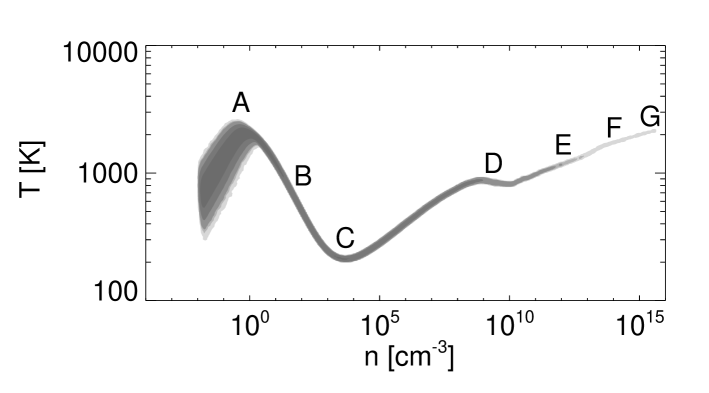
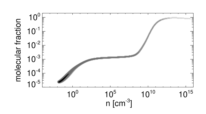
Figure 3.— (Top) Gas distribution in the temperature-density phase space in a spherical collapse problem. The indicated characteristic features are explained as follows; (A) gas temperature reaches $\gtrsim 1000$K by virialization, and hydrogen molecules are formed by two-body processes, (B) molecular hydrogen cooling brings the gas temperature down to 200 K, (C) the H₂ cooling rate saturates and becomes close to the density-independent, LTE value, (D) three-body reactions kick in and the gas becomes fully molecular, (E) the line cooling rate decreases as the density increases because of the cloud’s opacity, (F) collision-induced emission becomes a dominant cooling process, and (G) H₂ dissociation begins at $T\sim 2000$K. (Bottom) The molecular fraction $f_{\rm H2}$ of the gas. The increase in the fraction at A, D, a plateau at C$\rightarrow$D, and the temporal decrease owing to dissociation at G are clearly seen in this plot.

Previous three-dimensional simulations of primordial gas cloud formation were hampered by the complexity of calculating line opacities and the reduction of the resulting cooling rate. The maximum resolution, in terms of gas density, achieved in these simulations was thus $\sim 10^{10}{\rm cm}^{-3}$, where the assumption of optically thin cooling breaks down. With the novel technique described in Section 3.3, our simulations can follow the evolution of a primordial gas cloud to $n_{\rm H}\sim 10^{16}{\rm cm}^{-3}$, nearly six orders of magnitude greater than previous three-dimensional calculations reliably probed. To study the detailed evolution of a proto-stellar “seed” beyond $n_{\rm H}\sim 10^{16}{\rm cm}^{-3}$ , we would need to implement a few more physical processes, as explained in Section 3.5.

An important quantity we measure is the optically-thick line cooling rate, which serves as a critical check of our numerical implementation. Fig. 4 shows the normalized H₂ line cooling rate against local density. We use an output at the time when the central density is $n_{\rm c}=10^{14}{\rm cm}^{-3}$. In the figure, we compare our simulation results with those from the full radiative transfer calculations of ON98 (open diamonds). Clearly our method works very well. The steepening of the slope at $n>10^{12}{\rm cm}^{-3}$, owing to the velocity change where infalling gas settles gradually onto the center, is well-reproduced. We emphasize that the level of agreement shown in Fig. 4 can be achieved only if all of the local densities (of chemical species), temperatures, and velocities are reproduced correctly.

Figure 4.— The cooling efficiency defined by $f=\Lambda_{\rm thick}/\Lambda_{\rm thin}$. The open squares are the results from the one-dimensional calculation of Omukai & Nishi (1998). We plot the efficiency as a function of local density at the time when the central density is $n=10^{14}{\rm cm}^{-3}$.

5. Cosmological simulations

It is important to study the formation of primordial stars using a proper set-up, starting from realistic initial conditions. To this end, we have run a cosmological simulation adopting the concordance $\Lambda$CDM cosmology with matter density $\Omega_{m}=0.26$, baryon density $\Omega_{\rm b}=0.04$, cosmological constant $\Omega_{\Lambda}=0.7$, and expansion rate at the present time $H_{0}=70$km s^-1 Mpc^-1. The power spectra of the initial density fluctuations for baryons and dark matter are calculated by the Boltzmann code of Sugiyama (1995). In the examples discussed below, the power spectra were normalized to $\sigma_{8}=0.9$, consistent with the first year WMAP results, but slightly larger than the recent estimate of Spergel et al. (2006), based on their third year data-set. Everything else being equal, a smaller value of $\sigma_{8}$ will shift structure formation to slightly lower redshifts. The main purpose of our present investigation is to study the physics of gas collapse to high densities and fragmentation in dark matter halos. These processes will be unaffected by a shift in $\sigma_{8}$, although the cosmic time corresponding to the evolution we model would be different, as would the abundance of the halos and stars at a given redshift.

In order to avoid spurious clumping in the initial particle set-up, we use “glass” particle distributions (White 1996). Further details on the initial conditions are found in Yoshida, Sugiyama & Hernquist (2003). We use a simulation volume of $0.3$ Mpc on a side. Starting from a low resolution simulation, we select the most massive halo at $z=15$ in the volume and apply a hierarchical zoom-in procedure (e.g. Navarro & White 1993; Tormen et al. 1997; Gao et al. 2005) to the region surrounding the halo, so that progressively higher mass resolutions are realized. In the highest resolution part of the the initial conditions, the dark matter particle mass is 0.0944 $M_{\odot}$ and that of gas particles is 0.0145 $M_{\odot}$. In order to achieve an even higher mass resolution, we progressively refine the gas particles using the method of Kitsionas & Whitworth (2002) and Bromm & Loeb (2003) as the gas cloud collapses. We do this refinement so that a local Jeans length is always resolved by fives times the local SPH smoothing length. With this technique, we achieve a mass resolution of $m_{\rm p}=60M_{\oplus}$, where $M_{\oplus}$ denotes the Earth mass, at the last output time. For the study of cloud fragmentation at intermediate densities $n_{\rm H}=10^{9}-10^{11}{\rm cm}^{-3}$, we carry out two simulations; one with the refinement technique and the other without it, to verify that temporal perturbations caused by refinement do not affect the results presented in Section 5.2.

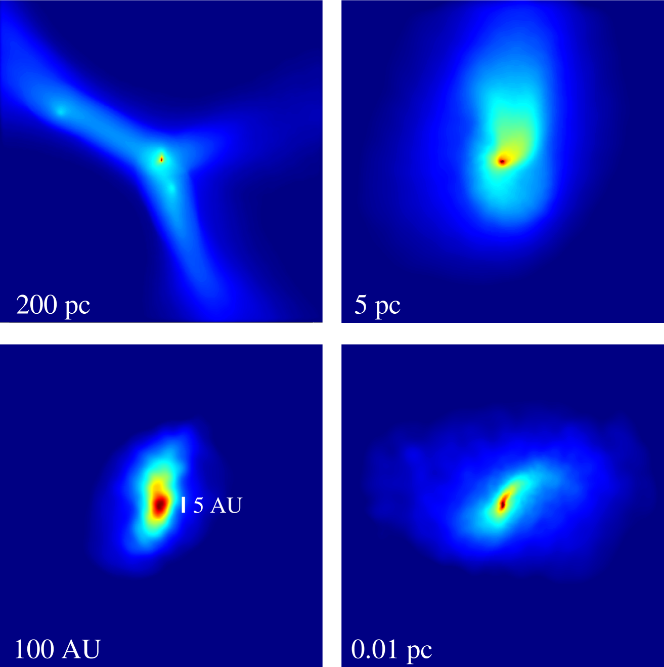
Figure 5.— Projected density distribution for our cosmological simulations at a redshift $z\approx 19$. The physical side-length is indicated in each panel.

Figure 6.— Radial profiles for density, temperature, molecular fraction, and infall velocity at a redshift $z\approx 19$. The density is plotted as a function of distance from the center, whereas the other three quantities are plotted as a function of enclosed gas mass. The density profile is close to the power-law $\propto R^{-2.2}$. The characteristic features in the temperature profile (marked A-G) can be explained as in Fig. 4 (see also text).

5.1. Thermal evolution of the proto-stellar gas cloud

In our $\Lambda$CDM simulation, the first gas cloud is formed at the center of a dark matter halo with a mass of $6\times 10^{5}M_{\odot}$. The halo is located at the intersection of filamentary structures at a high-density peak. Fig. 5 shows the projected gas density around the proto-stellar gas cloud. At the output time, the density of the cloud core has reached $\sim 3\times 10^{15}{\rm cm}^{-3}$. The four panels in Fig. 5 show progressively zoomed-in views of the central regions, with the physical dimension indicated in each panel (clockwise from 200 parsec to 100 AU). In the lower-left panel, we compare the size of the cloud core with a solid bar which indicates a length of 5 astronomical units! The central part in the top-right panel has a mass of $\sim 300M_{\odot}$ with an approximate diameter of $\sim 1{\rm pc}$; this region is self-gravitating and undergoing run-away collapse. In the bottom-right panel, the central darkest area is nearly fully molecular with a mass of about $1M_{\odot}$. Finally the darkest region in the bottom-left panel has a mass of $\sim 0.01M_{\odot}$, which is completely opaque to molecular lines and is cooling by CIE.

Fig. 5 shows the radial profiles of density, temperature, velocity, and molecular fraction at the final output time. Except for the density profile which is shown as a function of radius (note the x-axis is in astronomical units), the mass coordinate (enclosed gas mass) is used for the horizontal axis. Although the plotted profiles are for a single output time, the gas evolution can indeed be easily inferred from them, because the collapse time scales as $\propto 1/\sqrt{n}$, leaving the profiles of the outer region almost unchanged while the central parts collapse further. The density profile evolves self-similarly approximately as a power-law with $n\propto r^{-2.2}$ (dashed line in the top-left panel), being consistent with previous one-dimensional and three-dimensional simulations.

The characteristic features of the temperature profile are understood by various physical processes as we discussed already in the spherical collapse simulation. Virialization brings the gas temperature to above 1000 K, and hydrogen molecules are formed by two-body reactions (point A in the top-right panel of Fig. 5). The cloud cools by H₂ cooling (B) and the gas temperature is lowered to about 200 K (C). There, the gas density is $\sim 10^{4}{\rm cm}^{-3}$, beyond which the H₂ rotational level population approaches that of LTE. Then, the cooling rate per molecule becomes density-independent, and radiative cooling is much less efficient than in the low density limit. This is the so-called loitering regime (Bromm et al. 2002), and further collapse is induced dynamically when the cloud becomes Jeans-unstable. To see the onset of run-away collapse, we compare the enclosed gas mass with the locally estimated Bonnor-Ebert mass (Bonnor 1956; Ebert 1955):

$$M_{\rm BE} = \frac{m_{1}c_{\rm s}^{4}}{G^{3/2}P_{o}^{1/2}},$$ (46)

$$\approx 20M_{\odot}T^{3/2}n^{-1/2}\mu^{-2}\gamma^{2}\,,$$

where $m_{1}$ is the first maximum mass of the solution for the isothermal Lane-Emden equation (see, e.g. Stahler & Palla 2004), and $\mu$ and $\gamma$ denote the mean molecular weight and adiabatic index, respectively. We approximate the external pressure by its local value taken from the radial density and temperature profiles. (Note that $M_{\rm BE}$ evaluated in this manner is essentially the same as the local Jeans mass.) We find that the enclosed gas mass exceeds the Bonnor-Ebert mass at $M\sim 200M_{\odot}$. This is the characteristic mass of the collapsing gas cloud. We see in Fig. 5 that the temperature rises below this mass scale, showing clearly the onset of collapse and heating by contraction (Point C). The $200M_{\odot}$ cloud is now self-gravitating, being essentially decoupled dynamically from the host dark matter halo.

Three-body reactions convert most of hydrogen into molecules (D in the top-right panel). As the molecular fraction profile (bottom-left panel) shows, the central 1-2$M_{\odot}$ becomes fully molecular through these rapid reactions. Cooling by H₂ lines soon saturates because of gas opacity (E). When the core density reaches $\sim 10^{14}{\rm cm}^{-3}$, H₂ line cooling becomes very inefficient, but CIE cooling kicks in (region F). At higher densities, the gas temperature is maintained at $\sim$ 2000K, whereby dissociation of hydrogen molecules effectively absorbs heat input from contraction and dissipation of gravitational energy (G). Dissociation already commenced in the innermost region at the plotted output time, as is clearly seen in the molecular fraction profile at $M_{\rm enc}<0.1M_{\odot}$.

5.2. Thermal instability and fragmentation

It is an outstanding question whether or not primordial gas clouds are subject to thermal instability and fragment into multiple objects. Fragmentation could be manifested in various forms because it depends on the cloud geometry, thermal history, interaction with ambient matter, etc. Here, we focus on fragmentation of a primordial gas cloud collapsing in a CDM halo, with properties as found in our cosmological simulation. In our simulation, we find that the central gas cloud does not break up into multiple objects but remains intact as a single entity until the last output time. To study cloud fragmentation in detail and more generally, we examine the stability of the gas against thermal instability.

A well-known stability criterion is the so-called Field criterion:

$$\rho_{0}\left(\frac{\partial L}{\partial\rho}\right)_{T}-T_{0}\left(\frac{\partial L}{\partial T}\right)_{\rho}<0,$$ (47)

where $L$ is the energy loss rate per unit mass (Field 1965). Because the molecular hydrogen cooling rate is density-independent at high densities, and has a steep temperature dependence $\propto T^{\alpha}$ with $\alpha>1$ at $100<T[{\rm K}]<10000$ (see Fig. 1), the Field criterion is satisfied for primordial gas in this region for a fixed molecular fraction. Thermal instability can also be driven by a change in chemical composition, such as ionization/recombination (Defouew 1970; Goldsmith 1970) or molecule formation/dissociation (Yoneyama 1973). Sabano & Yoshii (1977) and Silk (1983) suggest that primordial gas can be chemo-thermally unstable. Chemo-thermal instability can be triggered when a rapid increase in the coolant fraction (H₂ molecules) induces efficient cooling and condensation, leading to an enhanced production of molecules via three-body reactions. There are two proposed regimes where the chemo-thermal instability can be triggered: one at $n\sim 10^{10}{\rm cm}^{-3}$ where three-body reactions make the overall gas cooling very efficient, and the other at $n\sim 10^{15}{\rm cm}^{-3}$ where collision-induced emission cooling comes into play.

Previously, ABN02 concluded that gas clouds do not fragment because of efficient turbulent mixing. Using one-zone calculations, Omukai & Yoshii (2003) conclude that the cloud core becomes unstable, but does not fragment because the cloud is already compact. Ripamonti & Abel (2004) study the thermal instability in the high density regime and argue that fragmentation is unlikely to occur. None of these previous works provide definitive answers, unfortunately. The high-resolution simulation of ABN02 employs the optically-thin approximation for H₂ cooling, and thus their results do not provide accurate estimates for relevant quantities at densities above $n>10^{10}{\rm cm}^{-3}$, whereas the other studies based on zero- or one-dimensional calculations suffer from the fact that fragmentation is intrinsically a three-dimensional problem. We are able to, for the first time, directly address this issue using a three-dimensional simulation with sufficient mass- and “physical” resolution in a fully cosmological context.

We follow Omukai & Yoshii (2003) to investigate the stability of the gas cloud core against isobaric perturbations. For perturbations in temperature, density, and molecular fraction, $\delta T,\delta\rho,\delta x\propto\exp(\omega t)$, under the constraint $\delta P=\delta T+\delta\rho+\delta x=0$, linear stability analysis yields the dispersion relation

$$A\omega^{2}+B\omega+C=0,$$ (48)

where

$$A=1+\frac{6-f}{2(2-f)},$$ (49)

$$B=\frac{\mu m_{p}}{kT}(TL_{T}-\rho L_{\rho}-L)-\frac{\mu\chi}{2kT}(TF_{T}-\rho F_{\rho}-F)-A\left(F_{f}+\frac{\mu}{2}\rho F_{\rho}+\frac{\mu F}{2}\right),$$ (50)

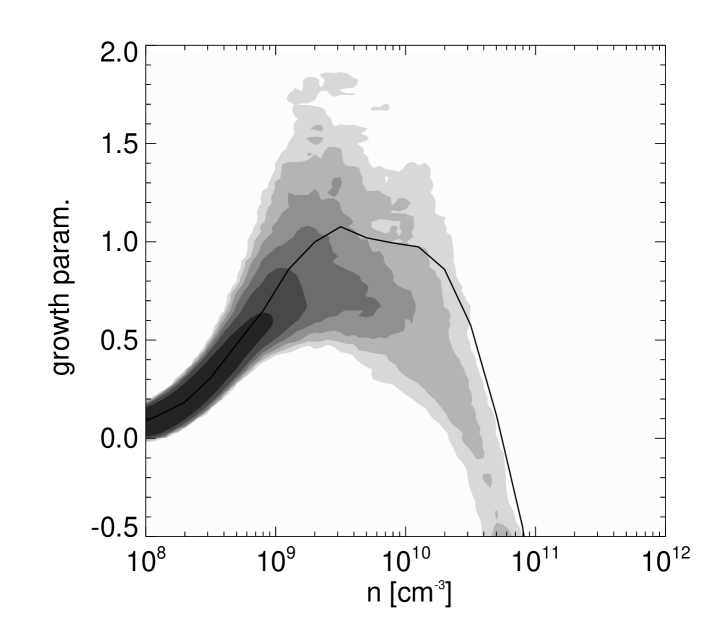
Figure 7.— The instability growth parameter $Q$ as a function of gas density. The shaded contour shows the distribution of the cloud core gas at a time when the central density is $\sim 10^{12}{\rm cm}^{-3}$. The thick solid line shows the evolution of the most dense particle in this $Q-n$ plane.

and

$$C = -\frac{\mu m_{p}}{kT}(TL_{T}-\rho L_{\rho}-L)\left(F_{f}+\frac{\mu}{2}\rho F_{\rho}+\frac{\mu F}{2}\right)$$ (51)

$$+ \frac{\mu m_{p}}{kT}\left(L_{f}+\frac{\mu}{2}\rho L_{\rho}+\frac{1}{6-f}L\right)(TF_{T}-\rho F_{\rho})$$

$$+ \frac{\mu}{2}F\left[\frac{\mu}{3-f/2}\left(\frac{1}{2}+\frac{\chi}{kT}\right)(TF_{T}-\rho F_{\rho})-\frac{\chi}{kT}\left(F_{f}+\frac{\mu}{2}\rho F_{\rho}+\frac{\mu F}{2}\right)\right]$$

$$- \frac{\mu}{(3-f/2)\;t_{\rm dyn}}(TF_{T}-\rho F_{\rho}).$$

In the above expressions, $f$ is the molecular fraction ($f=1$ for a fully molecular gas), $\mu=2/(2-f)$, $F=df/dt$ is the net formation rate of hydrogen molecules, and $L$ is the rate of energy loss per unit mass. Subscripts denote the respective partial derivatives. We have defined the local dynamical time

$$t_{\rm dyn}=\sqrt{\frac{3\pi}{32G\rho}}.$$ (52)

The dispersion equation (48) has a positive real root (a growing mode solution) if and only if $C<0$, because $A$ is positive by definition. Furthermore, for perturbations to grow in a gravitationally collapsing gas, the characteristic growth timescale $t_{\rm g}\propto 1/\omega$ must be shorter than the dynamical time $t_{\rm dyn}$. Hence, we define the growth parameter

$$Q=\frac{t_{\rm dyn}}{t_{\rm g}}=\omega t_{\rm dyn}.$$ (53)

If $Q>1$, perturbations are expected to grow faster than the gravitational contraction of the cloud (Omukai & Yoshii 2003; Ripamonti & Abel 2004).

Fig. 5.2 shows the growth parameter evaluated locally for all the gas elements at the time when the central density is $n_{\rm c}=10^{12}{\rm cm}^{-3}$. We also show the evolutionary track for the cloud core by the solid line. We see that a part of the gas cloud is in the unstable region where $Q>1$. However, $Q$ never becomes much larger than unity. It is indeed less than 1.5 for almost all the gas. Omukai & Yoshii (2003) argue that $Q$ must be significantly larger than unity for a gas parcel to break up into multiple objects. This is because the size of the cloud, $l_{\rm c}\sim c_{\rm s}t_{\rm dyn}$, must be much larger than the length of growing perturbations $l_{\rm p}\sim c_{\rm s}t_{\rm g}$. In other words, while a gas parcel can become thermally unstable, for the gas to break up into multiple objects, $Q$ must be at least larger than two so that the perturbations can grow before the region gravitationally contracts. Fig. 5.2 shows that the cloud center never enters the regime $Q>2$. Our results therefore support the conjecture of Omukai & Yoshii that the cloud becomes chemo-thermally unstable but evolves into a single object, because the cloud is already too compact.

We do the same analysis at the time when the cloud core enters the high-density regime. Evaluating equations (48)-(51), we find that the gas is always stable. To see this more clearly, we show the gas distribution in a thermodynamic phase diagram in Fig. 5.2. We indicate the region where $Q>0$ by grey contours. For estimating the value of $Q$ as a function of density and temperature, we calculate $f_{\rm H_{2}}$ assuming chemical equilibrium. We solve the cubic equation for the equilibrium molecular fraction

$$k_{22}(1-f)^{3}n^{3}+\frac{1}{2}k_{23}f(1-f)^{2}n^{3}=\frac{1}{2}k_{11}f(1-f)n^{2}+\frac{1}{4}k_{24}f^{2}n^{2},$$ (54)

where $k_{i}$ denote respective reaction rates tabulated in the Appendix. While the assumption of chemical equilibrium does not strictly hold in all the plotted range of density and temperature, it is indeed a good approximation for the relevant region where the actual gas evolutionary track lies. As clearly seen in Fig. 5.2, the gas never approaches an unstable region. It appears that, since the cooling rate is larger at higher density and/or at higher temperatures (see the temperature dependence of CIE cooling in Fig. 3.4), the gas evolutionary track circumvents the instability region. It is implausible that a gas parcel enters the instability region from the lower temperature side, because the cause of the instability is radiative cooling, which always tend to bring the gas temperature downward. We further argue that, because dissociation of hydrogen molecules occurring at $T>2000$K effectively absorbs the heat input by contraction and thermalization, the gas evolves approximately isothermally around $T\sim 2000$K until full scale dissociation is completed, and the temperature cannot increase much without the density increasing. We therefore conclude that fragmentation owing to thermal instability does not take place in this regime either.

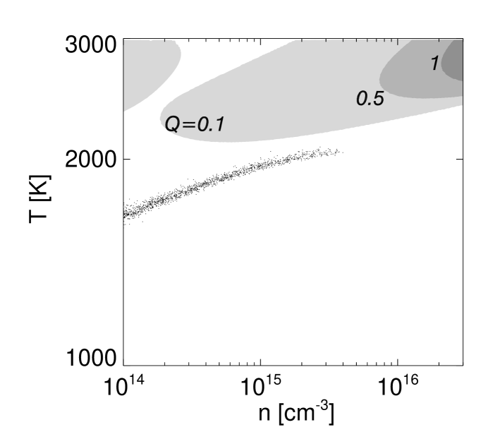
Figure 8.— Stability analysis in the high-density regime. We plot the distribution of gas in the cloud core in the temperature-density phase space. The shaded regions indicate regions with $Q=0.1,0.5,1$ from light to dark grey, respectively. The gas does not enter the instability region.

5.3. Stability against gravitational deformation

Gas fragmentation could be triggered if a cloud is significantly flattened (Tohline 1981; Miyama et al. 1984; Tsuribe & Inutsuka 1999; Bromm, Coppi, Larson 1999) or if it contracts into filamentary structures (Uehara et al. 1996; Nakamura & Umemura 2001). Although Bromm et al. (1999) present a particular case which yields a disk-structure, their simulation is set up as such, by imposing an initial spin. In cosmological simulations, primordial gas clouds with such shapes are not generally found (Abel et al. 2002; Yoshida et al. 2003). There are two important mechanisms that lead to cloud fragmentation; one is the growth of deformation during collapse and the other is rotation-induced fragmentation. While these two mechanisms are, in general, coupled to each other, we here examine each effect separately. We first show that the dense, collapsing gas cloud formed with $n_{\rm H}\sim 10^{4}{\rm cm^{-3}}$ would not fragment again at higher densities. The collapse of the dense core proceeds in a self-similar manner. This so-called Larson-Penston-type self-similar solution is known to be unstable to non-spherical deformation if $\gamma=d{\rm log}P/d{\rm log}\rho$ is less than the critical value, $\gamma_{\rm crit}=1.097$ (Hanawa & Matsumoto 2000; Lai 2000). An unstable core elongates by this instability and eventually fragments. Let us define the core’s elongation as ${\cal E}\equiv(b-a)/a$, where $a$ and $b$ are short and long axis lengths, respectively. The growth rate of the elongation $\nu=d{\rm log}{\cal E}/d{\rm log}{\rho}$ is calculated by Hanawa & Matsumoto (2000) and Lai (2000) using linear perturbation theory.

Figure 9.— Linear stability analysis for deformation growth. We plot the predicted evolution of the elongation ratio ${\cal E}$ for the core (solid line). The evolutionary track of the core stays below ${\cal E}=1$ after the first run-away collapse at $n_{\rm H}\sim 10^{4}{\rm cm}^{-3}$, suggesting that the core is stable against deformation to filamentary structure. The dashed line shows the evolution of the effective ratio of specific heats, and the dotted line is the critical value $\gamma_{\rm crit}=1.097$ from linear theory.

Using the simulation outputs, we calculate the effective ratio of specific heats $\gamma=d{\rm log}P_{\rm c}/d{\rm log}\rho_{\rm c}$ at the density maximum as a function of density. The evolution of the core elongation is then calculated as

$${\cal E}={\cal E}_{0}\;{\rm exp}\left(\int_{n_{\rm H,0}}^{n_{\rm H}}\nu(n_{\rm H}^{\prime})\;{\rm d}\ln n_{\rm H}^{\prime}\right)$$ (55)

for the initial elongation ${\cal E}_{0}$ at $n_{\rm H,0}$. In Fig. 5.3, we show the evolution as a function of the central number density. The initial state is taken at the maximum of ${\cal E}$ around $10^{4}{\rm cm^{-3}}$, where the first run-away collapse begins. Early in the evolution ($n_{\rm H}<10^{9}{\rm cm^{-3}}$), $\gamma$ exceeds $\gamma_{\rm crit}$, and the elongation decays; the core becomes rounder. With the onset of three-body H₂ formation, $\gamma$ starts decreasing and falls slightly below $\gamma_{\rm crit}$. There, the elongation grows but only slowly. As is seen in Fig. 5.3, it at most recovers the initial value ${\cal E}_{0}$. Since the effective $\gamma$ gradually increases again at $n>10^{10}{\rm cm}^{-3}$ when H₂ line cooling becomes inefficient, the deformation growth rate decreases. We thus conclude that the core must be stable initially and remains stable to this mode of fragmentation throughout the collapse, as is indeed the case in our simulation (see Fig. 5).

Next, we examine the effects of rotation. Tohline (1981) and many subsequent works (e.g. Tsuribe & Inutsuka 1999) conclude that basically two parameters, the cloud’s initial ratio of thermal to gravitational energy ($\alpha_{0}$) and the initial ratio of rotational to gravitational energy ($\beta_{0}$), determine whether or not the cloud will eventually fragment, for a given adiabatic exponent $\gamma$. Here, the parameters are defined as, respectively,

$$\alpha_{0}=\frac{5c_{\rm s}^{2}R_{0}}{2GM},\;\;\;\beta_{0}=\frac{\Omega_{0}^{2}R_{0}^{3}}{3GM}.$$ (56)

Note that the latter quantity is essentially the degree of rotation support (see Section 5.5 below). Tsuribe (2002) investigated a particular case for $\gamma=1.1$, which is close to the actual value for primordial gas, and concluded that the stability criterion is roughly given by $\alpha_{0}>0.3$ for $0<\beta_{0}<0.3$. (Note that the stability region does not differ much for a gas cloud with a constant initial density or for a gas cloud with central condensation [Tsuribe 2002].) We calculate these quantities at the time when the first run-away collapse begins, namely when the core density is $\sim 10^{4}{\rm cm}^{-3}$ and the temperature is $\sim 200$K (Point C in Fig. 5). We find $\alpha_{c}=1.0$ and $\beta_{c}=0.1$, which satisfies the stability condition. In summary, the gas cloud in our cosmological simulation is found to be stable against deformation and rotation-induced fragmentation. We have validated the numerical results using analytical stability criteria.

Figure 10.— Instantaneous gas mass accretion rate around the proto-stellar core (solid curve). We evaluate equation (57) and plot it as a function of enclosed gas mass. For reference, the dashed line shows the accretion rate obtained by Omukai & Nishi (1998) using their post-singularity, self-similar solution. The dotted line is the critical mass accretion rate given by equation (65).

5.4. Gas mass accretion rate

We have seen that the prestellar cloud does not fragment into multiple clumps. Since the entire cloud has a much larger mass than the proto-stellar “seed”, the protostar will evolve in an inside-out manner, by accreting a large quantity of surrounding gas. The rate of accretion of the infalling gas is among the most important quantities in proto-stellar evolution. Since the late time evolution of the protostar itself affects the matter accretion rate, we are not able to measure the true mass accretion rate onto the protostar directly. Nevertheless, the instantaneous accretion rate likely provides a good estimate. In Fig. 5.3, we show the instantaneous gas mass accretion rate at the last output time

$$\dot{M}=4\pi\rho\;r^{2}v_{\rm rad}(r)$$ (57)

using again the mass coordinate. We compare our result with that of ON98 which is derived from the post-singularity self-similar solution (Yahil 1983). The model accretion rate of ON98 has a shallower slope (i.e., larger accretion rate in the outer regions) than that of our simulation. This is reasonable because the ON98 model is based on the Larson-Penston type self-similar solution that predicts higher infall velocities at large distances because of the assumption of the solution itself; the velocity difference owes to the initial conditions and boundary effects, which are self-consistently calculated in our simulation.

A simple, order of magnitude estimate for the mass accretion rate is given as a function of sound speed as

$$\dot{M}\sim\frac{c_{s}^{3}}{G},$$ (58)

and thus it is large for a high temperature gas. For $T\sim 1000$ K, the above estimate yields $\sim 10^{-3}M_{\odot}{\rm yr}^{-1}$, similar to the simulation result. It is illustrative to compare this value with that in present-day star-forming regions which have $T\sim 10$ K. The temperature difference naturally explains the much larger accretion rate, by more than two orders of magnitude, for the primordial case. Intriguingly, the overall feature of the accretion rate shown in Fig. 5.3 can be explained qualitatively from the temperature profile. The gradual increase at $M_{\rm enc}=100-1000M_{\odot}$ corresponds to the gradual temperature increase shown in the top-right panel in Fig. 5. The slight shallowing at $M_{\rm enc}\sim 10M_{\odot}$ corresponds to the temperature “dip” where three-body reactions promote molecule formation. Inside the radius, $M_{\rm enc}<10M_{\odot}$, the temperature rises again, and the accretion rate increases as well. The decline at the inner-most part is simply because of the output timing. At this time, the radial velocity gradually decreases towards the center (Fig. 5); i.e. a radiative shock has not yet formed. In the outer part, $M_{\rm enc}>1000M_{\odot}$, the increasing accretion rate owes to gravitational pull by the host dark matter halo, which is not seen in cloud evolution calculations without dark matter.

The instantaneous accretion rate is larger than ABN02 found over the entire plotted mass range. While the small accretion rate at $M_{\rm enc}<10M_{\odot}$ in ABN02 can be understood as a result of over-cooling (see Fig.2 in ABN02), it is unclear why the large-scale ($M_{\rm enc}\gtrsim 100M_{\odot}$) mass accretion rates differ. It cannot be attributed to the degree of rotational support because we obtained quite similar rotation values to ABN02 (see the next section). To study this discrepancy further, we carry out two controlled simulations by embedding a primordial gas within an NFW dark matter halo similarly to the simulation presented in Section 4. For one case we set $f_{\rm b}=0.16$, consistent with our $\Lambda$CDM cosmology, whereas for the other case, we set $f_{\rm b}=0.05$, that is the value adopted in the standard cold dark matter simulation with $\Omega_{\rm m}=1$ of ABN02. For both cases we assign zero velocities initially and let the gas cloud collapse in the halo’s potential with the same mass. We measured the resulting mass accretion rates at the time when the central density reaches $n_{\rm c}=10^{15}{\rm cm}^{-3}$. We find, interestingly, that the low baryon fraction case agrees well with the result of ABN02. The overall cooling time in the low baryon fraction case is longer than in the other one and hence collapse takes place more slowly. In the high baryon fraction case, external pressure from the ambient gas at the onset of collapse may also affect the accretion rate (Hennebelle et al. 2004; Motoyama & Yoshida 2003). Given the insignificant difference of up to a factor of a few, we do not discuss the discrepancy further in the present paper. Recently, O’Shea & Norman (2006a,b) performed a series of cosmological simulations to examine various environmental effects, such as large-scale local density and halo formation epoch, on the instantaneous gas mass accretion rate. They indeed find a substantial variation in accretion rate among different halos. We mention that very different cosmological environments, such as those realized in the early large-scale structure simulation of Gao et al. (2005) could have a noticeable impact on the mass accretion rate.

5.5. Angular momentum

The gas cloud starts collapsing with a finite amount of angular momentum (AM), and thus it is expected to spin-up gradually as it contracts, unless there are some mechanisms to transfer AM. Rotational support of the gas may play an important role in the process of accretion. To first order, we expect that mass accretion continues only if rotation does not halt collapse; i.e. if the angular momentum of the gas is small. We calculate the specific angular momentum profile around the protostar at the final output time. Fig. 5.5 shows the profile as a function of enclosed gas mass. The power-law profile is typical for gravitationally collapsed objects (Bullock et al. 2001; van dens Bosch et al. 2002). The AM profile’s shape and even the amplitude are quite similar to the one found in the simulation of ABN02 over the entire plotted range. The degree of rotational support defined as

$$f_{\rm r}=\frac{L_{\rm sp}/r}{V_{\rm kep}},\;\;\;V_{\rm kep}=\sqrt{\frac{GM}{r}},$$ (59)

is shown by the dashed line. Here, $L_{\rm sp}$ is the specific AM of the gas within radius $r$, and $V_{\rm kep}$ is the Kepler velocity at that radius. It is about 40-50% for $M_{\rm enc}=0.01-1000M_{\odot}$, and rotation is not (yet) able to stop the gas inflow. We have also measured $f_{\rm r}$ at previous output times and found that $f_{\rm r}$ has been monotonically increasing at small radii. To understand the reason for the characteristic AM profile, i.e., why low angular momentum material resides in the central regions, we examine two quantities.

First, we make a conjecture that the region with little angular momentum collapses first. By measuring the probability distribution of specific AM in the cloud before the onset of collapse, we show that this is indeed the case in our simulation. At a time when the maximum density reaches $10^{4}{\rm cm}^{-3}$, we define the “core” as the region where the density is larger than half that of the center. The center is defined to be the position of the most dense particle. We then calculate the specific angular momentum with respect to random points within the core, by taking a fluid parcel of mass $0.1M_{\rm Jeans,core}=30M_{\odot}$ around the points. The resulting probability distribution is shown in Fig. 5.5. There, the arrow indicates the value for the “true” center that collapses first and becomes the densest part in the later output time. We interpret this, together with the specific AM distribution, as evidence that regions with low angular momentum collapse fast in the (weakly-)turbulent medium. There is alway a central core within which density fluctuations are erased by soundwaves (hence having a size $\sim c_{\rm s}t$), and there is also an AM distribution within it.

We further examine the evolution of AM in detail, making use of the Lagrangian nature of the SPH method. We trace the inner-most particles and calculate the evolution of the specific AM. We mark gas particles according to their mass coordinate at the final output time and divide them into four shells. We then keep track of the positions and velocities of the marked particles at earlier output times. At each output time, we shift the spatial coordinate such that the “true” central particle is always at the origin of the coordinate. (We note that the specific AM profile varies considerably if we define the center as the most dense region at each output time.) Fig. 5.5 shows the evolution of the specific angular momentum for the four mass shells. As is clearly seen in the right panel of Fig. 5.5, the specific angular momentum of each mass shell is well-conserved, while the mean radii decreased by a factor of 3-5. This causes the gradual increase of rotational support in the inner region as discussed previously.

Figure 11.— Specific angular momentum profile in the gas cloud. The dashed line shows the degree of rotational support as defined by equation (59). It is about 40-50% for the entire cloud.

In order to verify that numerical viscosity did not significantly influence our results, we have explicitly checked the torque exerted on the gas cloud. In SPH, the equation of motion for each gas particle is expressed as

$$m\frac{{\rm d}v}{{\rm d}t}=F_{\rm grav}+F_{\rm pressure}+F_{\rm visc}\,,$$ (60)

where the last term denotes the force owing to artificial viscosity (see Springel 2005 for exact expressions of each term). Then the torque $N={\rm d}L/{\rm d}t$ exerted on a gas cloud consisting of $M$ particles can be reduced to a sum of three components:

$$N = \sum_{i}^{M}r_{i}\times m\dot{v}_{i}$$ (61)

$$= \sum_{i}^{M}r_{i}\times(F_{\rm grav}+F_{\rm pressure}+F_{\rm visc})_{i}=N_{\rm grav}+N_{\rm pressure}+N_{\rm visc}\,.$$

We store the forces on each particle in output files and calculate explicitly all the terms in equation (61). We find that the dominant torques are $N_{\rm grav}$ and $N_{\rm pressure}$ throughout the evolution. Within the collapsing gas cloud ($M_{\rm enc}<200M_{\odot},r<0.1{\rm pc}$), $N_{\rm grav}$ and $N_{\rm pressure}$ are completely dominant, and $N_{\rm visc}$ is always less than 10% of $N_{\rm pressure}$ for all the mass shells. Note that a small amount of dissipation by weak shocks is expected, because there are some fluid elements that are moving at transonic velocities, as found in the adaptive mesh refinement simulations of ABN02. We have also performed the spherical collapse test of Norman, Wilson & Barton (1980). We set up a rotating spherical cloud as in Norman et al. (see also Truelove et al. 1998); $M=1M_{\odot},R=7.01\times 10^{16}{\rm cm}$ and the initial rotation $\Omega=3.04\times 10^{-13}{\rm rad}\;{\rm sec}^{-1}$. We use a half million particles to represent the sphere. For an ideal (inviscid) fluid with no means of angular momentum redistribution, the specific AM distribution is conserved, and it takes a simple analytic form

$$M(<K)=M\left[1-\left(1-\frac{K}{\Omega R^{2}}\right)^{3/2}\right],$$ (62)

where $M(<K)$ is the mass of fluid elements that have specific AM less than K. We measure the distribution at the initial time and that after about one free-fall time. The AM distribution is found to be conserved rather well, with the deviation at the smallest mass scale being less than 20%. This is a similar level of agreement as found in, for example, the calculation of Truelove et al. (1998). Although a good level of AM conservation in this test is expected for a Lagrangian hydrodynamics code, our test results reassure that the artificial viscosity does not do any harm to angular momentum transport in dynamically collapsing gas spheres such as those studied in the present paper.

Figure 12.— (Left) Probability distribution of specific angular momentum in the core region when the first collapse is being triggered. The part that becomes the central region in the end has a small angular momentum initially (indicated by the solid arrow), whereas the temporal center (most dense region) before the collapse has a larger angular momentum of $\sim 0.03$ pc km/sec. (Right) Evolution of the ‘Lagrangian’ specific angular momentum with respect to the marked center of the gas cloud for four groups of gas elements that are labeled according to their final mass coordinates.

5.6. Evolution of the protostar

It is still beyond the capability of the current simulation code and architecture to directly follow the evolution of the protostar to the point where it settles onto the zero-age main sequence (ZAMS). We tackle this demanding problem by employing the scheme for protostellar evolution of Stahler, Shu, & Taam (1980a,b) as modified by Stahler et al. (1986a,b) and Omukai & Palla (2001; 2003). We assume that the gas accretion takes place in an approximately spherically symmetric manner. We use the mass accretion rate shown in Fig. 5.3 as an input to the protostellar evolution code. While this assumption may seem over-simplified, the gas mass accretion rate from our cosmological simulation provides a reasonable estimate for true accretion rates onto a protostar, at least for the initial accretion phase, because the central gas cloud is roughly spherical and the gas in the envelope is not yet in a disk structure. Moreover, the protostellar evolution calculations include various physics and thus will give a more self-consistent solution of the evolution of a protostar for a given mass accretion rate. We thus employ this method rather than use simple time-scale arguments as done by ABN02 and Bromm & Loeb (2004).

Briefly, the evolution of a protostar is treated as a sequence of a growing hydrostatic core with an accreting envelope. The core is assumed to be in hydrostatic equilibrium, and the ordinary stellar structure equations are applied. The structure of the accreting envelope is calculated with the assumption that the flow is steady for a given mass accretion rate. Only the inner envelope that is optically thick to continuum is included. The effects of radiation pressure are considered in constructing the structure of the envelope. The details of the calculation are found in Stahler, Palla, & Salpeter (1986a,b) and Omukai & Palla (2001; 2003).

We use the time-(equivalently, protostellar mass-)dependent accretion rate $\dot{M}_{\rm fid}$ derived from our simulation (Fig. 5.3). We refer to this rate as the fiducial rate hereafter. The evolution of the protostellar radius is shown in Fig. 5.6. as a function of the protostellar mass. Considering the possibility that some fraction of infalling matter stacks in the circumstellar disk or is ejected as an outflow, we also show cases of accretion rates reduced from our fiducial value by a factor of 2/3 and 1/3.

Initially, the Kelvin-Helmholz (KH) time $t_{\rm KH}$, which is the timescale for a star to lose its thermal energy by radiation, is longer than the accretion timescale $t_{\rm acc}$ because the temperature of the protostar is low and its opacity owing to free-free absorption is large ($\kappa_{\rm ff}\propto T^{-7/2}$). The accreted material simply piles up on the stellar surface without cooling. This phase is called the adiabatic accretion phase and lasts up to $M_{\ast}\sim 10M_{\sun}$. During this phase, the radius first increases linearly (in log scale) with the protostellar mass, and then remains almost constant at $100R_{\sun}$. This behavior can be explained as follows.

The protostellar radius in the adiabatic accretion phase depends on the protostellar mass and accretion rate as (Stahler et al. 1986a,b)

$$R_{\ast}\propto\dot{M_{\ast}}^{0.4}M_{\ast}^{0.3}.$$ (63)

The increase of the radius in the earliest phase of evolution is explained by the increasing mass and accretion rate shown in Fig. 5.3. This is partly because our mass resolution is limited, and hence the output time is slightly before the formation of an accretion shock. Also, adjustment from a somewhat arbitrary initial structure to the appropriate accretion phase produces somewhat complex behavior at $M_{*}<0.3M_{\odot}$. The accretion rate decays with mass as $\dot{M_{\ast}}\propto M_{\ast}^{-0.8}$ in the range $1M_{\odot}<M_{\ast}<10M_{\odot}$ in our fiducial model. Substituting this into the above relation, we see that the mass dependence of the radius almost cancels. This explains the approximate constancy of the radius in this range.

Figure 13.— Proto-stellar evolution. The assumed accretion rates are taken from our fiducial model $\dot{M}_{\rm fid}$ (solid), $(2/3)\dot{M}_{\rm fid}$ (dashed), $(1/3)\dot{M}_{\rm fid}$ (dash-dotted). The solid points indicate the time when hydrogen burning begins.

With increasing protostellar mass, increasing temperature in the stellar interior makes the opacity lower and the radiation diffuses out more easily. When the protostellar mass reaches $\sim 10M_{\odot}$, heat deposited in the interior is transported outwards by a luminosity wave, whose arrival to the surface makes the star swell suddenly (Stahler et al. 1986a,b). After that, the protostar enters the Kelvin-Helmholtz contraction phase. By losing thermal energy to radiation, the protostar shrinks as (Omukai & Palla 2003)

$$R_{\ast}\propto\dot{M_{\ast}}M_{\ast}^{-2}.$$ (64)

The interior temperature increases until the contraction is halted by nuclear burning.

Energy generation by the p-p chain is not sufficient to stop the contraction of the already massive star. When the central temperature reaches $10^{8}$K, hydrogen burning by the CNO cycle begins with a slight amount of C synthesized by He burning. The onset of hydrogen burning by the CNO cycle is marked by a solid circle in the figure. The energy generation by hydrogen burning halts contraction around $100M_{\odot}$, and the star reaches the ZAMS. The protostar relaxes to a ZAMS star eventually within about $10^{5}$ years from the birth of the protostellar seed. In our calculation, there is no sign that accretion is halted by stellar feedback although the radiation pressure onto the accreting matter is included. Even after its arrival onto the ZAMS, the star continues to accrete. In principle, the star can grow in mass during its entire lifetime. (Note that the accretion rate at the outer boundary is given as a boundary condition. The gas accretion is sustained because of this condition. See the discussion below.) The stellar mass would become greater than a few hundred solar masses during its main sequence lifetime ($\sim 3\times 10^{6}$ yrs) if we were to allow mass accretion to continue using our estimated accretion rate. This mass scale is similar to the total gas mass of the dense core. This coincidence is not by chance: since the stellar lifetime is longer than the free-fall time of the dense core ($\sim 3\times 10^{5}$ yrs for $n_{\rm H}\sim 10^{4}{\rm cm^{-3}}$), the whole core falls onto the star.

In order for the accretion to continue, the total luminosity of the protostar $L_{\rm tot}$, given by the sum of the luminosity from the stellar interior $L_{\ast}$ and that from the accretion shock $L_{\rm acc}=GM_{\ast}\dot{M}_{\ast}/R_{\ast}$, must not exceed the Eddington limit $L_{\rm Edd}=4\pi cGM_{\ast}/\kappa_{\rm es}$, where $\kappa_{\rm es}$ is the electron scattering opacity, the dominant source of opacity in the inner envelope. The total luminosity approaches the Eddington limit as the star approaches the ZAMS, decreasing the radius and increasing the luminosity. To reach the ZAMS, the mass accretion rate must be less than

$$\dot{M}_{\rm crit}\simeq\frac{(L_{\rm Edd}-L_{\rm ZAMS})R_{\rm ZAMS}}{GM_{*}},$$ (65)

where $R_{\rm ZAMS}$ and $L_{\rm ZAMS}$ are the radius and luminosity of the ZAMS star of mass $M_{\ast}$. The dependence of the critical accretion rate on stellar mass is very weak and becomes approximately constant at $\dot{M}_{\rm crit}\simeq 4\times 10^{-3}M_{\odot}{\rm yr}^{-1}$ (Omukai & Palla 2003). This means that once the star reaches the ZAMS, the luminosity remains always below the Eddington limit and the accretion continues unimpeded. In Fig. 5.3, we show the critical rate by the dotted line. Although the accretion rate is higher than the critical value in the early evolution, the total luminosity falls below the Eddington limit owing to the larger radius and smaller interior luminosity in that phase than a ZAMS star of the same mass. For the fiducial accretion rate, the accretion rate drops below the critical value at $M_{\ast}\simeq 30M_{\odot}$, well before the star reaches the ZAMS. Consequently, the total luminosity never exceeds the Eddington limit and accretion continues.

We also explored two other cases besides our fiducial model. For these cases, we attempt to model crudely the feedback effects from the protostar and the consequences of rotation by reducing the mass accretion rate from the original value. The formed protostar could launch a protostellar outflow if a small magnetic field is present initially (Machida et al. 2006). Some fraction of infalling matter in the envelope is eventually ejected as an outflow without falling onto the central star and the accretion rate onto the protostar is reduced. To this end, we use reduced accretion rates of $(2/3)\dot{M}_{\rm fid}$ and $(1/3)\dot{M}_{\rm fid}$. The overall evolution of these cases is similar to that of the fiducial case, but characteristic mass scales are shifted to somewhat lower values. For the case with $\dot{M}=(1/3)\dot{M}_{\rm fid}$, the protostar reaches the ZAMS when its mass is $\sim 60M_{\odot}$. In the case of disk accretion, not only the accretion rate, but also the surface boundary condition of the star is altered. For smaller accretion rates ($10^{-5}-10^{-4}M_{\odot}/{\rm yr}$), Palla & Stahler (1992) studied the cases of different boundary conditions, which correspond to spherical or disk accretion cases. Intriguingly, they showed that the evolutionary behavior is quite similar in both cases qualitatively; the star reaches ZAMS somewhat earlier in the disk accretion case.

In summary, the accretion is not halted by radiative feedback for the fiducial and reduced accretion rates. Note, however, that we only considered the inner envelope, which is optically thick to continuum. In the outer envelope, the Ly$\alpha$ opacity could be important for halting accretion (Doroshkevich & Kolesnik 1976; Tan & McKee 2004). The expansion of an Hii region might be an another possibility to hinder accretion (Larson & Starrfield 1971; Tan & McKee 2004). Since the expansion of an Hii region is quenched for a large accretion rate assuming spherical symmetry (e.g., Omukai & Inutsuka 2002), non-spherical effects must be included for evaluating the exact time behavior of the expansion of the Hii region. While these uncertainties remain in determining the exact mass-scale of the first stars, the fact that they are rather massive seems to be robust.

6. Summary and Discussion

We have developed numerical techniques to implement the required chemical and radiative processes for following the thermal evolution of primordial gases to very high densities. Using a cosmological simulation with hydrodynamics and chemistry, we have studied the formation and evolution of pre-stellar gas clouds in a $\Lambda$CDM universe. Our three-dimensional simulation for the first time resolves the inner $\sim 1M_{\odot}$ fully molecular core, allowing us to obtain correct density, temperature, and velocity structure around the primordial protostar. These quantities altogether yield an accurate gas mass accretion rate around the protostar that was uncertain in previous works. We have derived three important facts from our simulations: (1) the primordial gas cloud in a cosmological minihalo does not fragment, but yields a single proto-stellar seed, (2) the cloud core has a small angular momentum so that rotation does not halt the collapse, nor is a disk formed, and (3) the rate of accretion from the cloud envelope is large. From these facts, we conclude that the first stars are massive. By performing a proto-stellar evolution calculation, we derive that the protostar grows to $\sim 100M_{\odot}$ for the particular case found in our simulation. We derive the stellar mass for the first time from a self-consistent calculation of proto-stellar evolution, coupled with a cosmological simulation.

While we simulated only a single halo in detail, the particular case shows a convincing and plausible case for the formation of massive stars in early mini-halos in the CDM model. The fate of such massive primordial stars (Population III), whether or not they are commonly born in various environments, are of considerable interest. They are likely responsible for various feedback effects in the early Universe (Haiman, Rees, & Loeb 1997; Bromm, Yoshida, & Hernquist 2003; Yoshida, Bromm, & Hernquist 2004; see Ciardi & Ferrara 2005 for a review). Stars with mass $140-260M_{\odot}$ are believed to trigger pair-instability supernovae and expel all the processed heavy elements in the explosion (Bond, Arnett, & Carr 1984; Heger & Woosley 2002). It has also been suggested that less massive stars die as hypernovae (Umeda & Nomoto 2002), producing a quite different metal yield from the pair-instability case. Interestingly, the observed abundance pattern of extremely metal poor stars appears to favor the latter scenario (Umeda & Nomoto 2003; Frebel et al. 2005). Energetic supernovae are also destructive, being effective in evacuating the halo gas (Bromm, Yoshida & Hernquist 2003; Wada & Venkatesan 2003; Kitayama & Yoshida 2005) and possibly quenching further star-formation in that region. A single supernova would suffice to pollute a large volume of the interstellar matter from which very metal-poor stars might have been formed. Metal-enrichment by the first supernovae may also lead to the formation of ordinary stellar populations including low-mass stars (e.g. Mackey et al. 2003) if metal-enrichment is relatively confined within a small region. Intriguingly, Jimenez & Haiman (2006) argue that metal-mixing could be inefficient and that primordial stars are formed in galaxies at $z<5$.

Massive stars emit a large number of ionizing photons and can ionize a large volume of the intergalactic medium around them (Kitayama et al. 2004; Whalen et al. 2004). Recently, Yoshida (2006) carried out radiation-hydrodynamic calculations of early Hii regions and concluded that radiation from a massive Population III star can completely ionize the gas within the host halo, quenching further gas condensation and star-formation for a significant period of cosmic time. Both massive and very massive ($>300M_{\odot}$) stars likely leave a black hole remnant. It is plausible that the remnants become the seeds for supermassive black holes that power luminous quasars found at $z\gtrsim 6$ (Li et al. 2006, in preparation) and subsequently at lower redshifts (e.g. Di Matteo et al. 2005; Hopkins et al. 2005, 2006). Because bottom-up hierarchical structure formation is a generic prediction of the CDM model, it is natural to think that the early population stars affect and even set the initial conditions for primeval galaxy formation. It is important to explore feedback from the first stars in more detail under a proper cosmological set-up.

The prospects for detecting the first generation of stars appear promising. Supernovae resulting from the collapse of massive stars can be observed if they trigger gamma-ray bursts (GRBs). There is growing evidence that long duration GRBs are associated with energetic supernovae (e.g. Hjorth et al. 2003). Gou et al. (2004) suggest that the afterglow of high-redshift GRBs can be detected in X-rays. There are also a broad range of observations through which we can, in principle, indirectly observe star-formation at high redshifts, through, for example, angular fluctuations in redshifted 21 cm emission from intergalactic gas as stars reionize the Universe (see, e.g. Zaldarriaga et al. 2004; Furlanetto et al. 2004; Zahn et al. 2006), or from secondary anisotropies imprinted from stellar radiation on the CMB (e.g. McQuinn et al. 2005; Zahn et al. 2005).

Finally, we remark that it is still too early to definitely conclude the exact mass or mass range of the first stars. The actual mass accretion could take place in a more complicated manner than we assume. Feedback from the protostar itself can affect the dynamics and thermal evolution of the accreting gas. Ultra-violet radiation from the protostar likely affects the gas infall rate. However, primordial gas has a much smaller opacity because of the absence of dust, and thus radiation pressure is generally not important (Omukai & Inutsuka 2002). The effect of radiation pressure can also be reduced if protostellar outflows provide optically thin cavities through which photons can escape (Krumholz, McKee & Klein 2005). Future calculations of proto-stellar evolution need to include these feedback effects onto the infalling gas. Also, accurate modeling of disk accretion may be necessary in general cases (Tan & McKee 2004). Although our simulation is currently resolution-limited (rather than physics-limited), with the maximum density being still five orders of magnitude smaller than stellar densities, we foresee that it will be possible to carry out an ab initio calculation of the formation of primordial protostars in the near future.

NY thanks Fumitaka Nakamura, George Field, Simon Glover, Gao Liang, and Brian O’Shea for insightful discussions. The simulations were performed at the Center for Parallel Astrophysical Computing at Harvard-Smithsonian Center for Astrophysics, at the Center for Computational Cosmology at Nagoya University, and at the Data-Reservoir at the University of Tokyo. We thank Mary Inaba and Kei Hiraki for providing the computing resource at U-Tokyo. The work is supported in part by the Grants-in-Aid for Young Scientists (A) 17684008 (N.Y.), and by Young Scientists (B) 18740117, Scientific Research on Priority Areas 18026008 (K.O.) by the Ministry of Education, Culture, Science and Technology of Japan. This work was supported in part by NSF grants AST 03-07433 and AST 03-07690, and NASA ATP grants NAG5-12140, NAG5-13292, and NAG5-13381.

Table 1REACTION RATE COEFFICIENTS

	Reactions	Rate Coefficients (cm3s-1)	Reference
(1)	${\rm H}+e\rightarrow{\rm H^{+}}+2e$	$k_{1}=\exp[-32.71396786+13.536556\;(\ln T_{\rm e})$
		$-5.73932875\;(\ln T_{\rm e})^{2}+1.56315498\;(\ln T_{\rm e})^{3}$
		$-0.2877056\;(\ln T_{\rm e})^{4}+0.0348255977\;(\ln T_{\rm e})^{5}$
		$-0.00263197617\;(\ln T_{\rm e})^{6}+0.000111954395\;(\ln T_{\rm e})^{7}$
		$-2.03914985\times 10^{-6}\;(\ln T_{\rm e})^{8}]$	1
(2)	${\rm H^{+}}+e\rightarrow{\rm H}+h\nu$	$k_{2}=\exp[-28.6130338-0.72411256\;\ln T_{\rm e}$
		$-0.0202604473\;(\ln T_{\rm e})^{2}-0.00238086188\;(\ln T_{\rm e})^{3}$
		$-0.000321260521\;(\ln T_{\rm e})^{4}$
		$-0.0000142150291\;(\ln T_{\rm e})^{5}$
		$+4.98910892\times 10^{-6}\;(\ln T_{\rm e})^{6}$
		$+5.75561414\times 10^{-7}\;(\ln T_{\rm e})^{7}$
		$-1.85676704\times 10^{-8}\;(\ln T_{\rm e})^{8}$
		$-3.07113524\times 10^{-9}\;(\ln T_{\rm e})^{9}]$	1
(3)	${\rm He}+e\rightarrow{\rm He^{+}}+2e$	$k_{3}=\exp[-44.09864886+23.91596563\;\ln T_{\rm e}$
		$-10.7532302\;(\ln T_{\rm e})^{2}+3.05803875\;(\ln T_{\rm e})^{3}$
		$-0.56851189\;(\ln T_{\rm e})^{4}+0.0679539123\;(\ln T_{\rm e})^{5}$
		$-0.00500905610\;(\ln T_{\rm e})^{6}+0.000206723616\;(\ln T_{\rm e})^{7}$
		$-3.64916141\times 10^{-6}\;(\ln T_{\rm e})^{8}]$	1
(4)	${\rm He^{+}}+e\rightarrow{\rm He}+h\nu$	$k_{4r}=3.925\times 10^{-13}T_{\rm e}^{-0.6353}$
		$k_{4d}=1.544\times 10^{-9}T_{\rm e}^{-1.5}\exp(-48.596/T_{\rm e})\times[0.3+\exp(8.10/T_{\rm e})]$	1
(5)	${\rm He^{+}}+e\rightarrow{\rm He^{++}}+2e$	$k_{5}=\exp[-68.71040990+43.93347633\;\ln T_{\rm e}$
		$-18.4806699\;(\ln T_{\rm e})^{2}+4.70162649\;(\ln T_{\rm e})^{3}$
		$-0.76924663\;(\ln T_{\rm e})^{4}+0.08113042\;(\ln T_{\rm e})^{5}$
		$-0.00532402063\;(\ln T_{\rm e})^{6}$
		$+0.000197570531\;(\ln T_{\rm e})^{7}$
		$-3.16558106\times 10^{-6}\;(\ln T_{\rm e})^{8})$	1
(6)	${\rm He^{++}}+e\rightarrow{\rm He^{+}}+h\nu$	$k_{6}=2\times k_{2}(T_{\rm e}/4)$	1
(7)	${\rm H}+e\rightarrow{\rm H^{-}}+h\nu$	$k_{7}=1.4\times 10^{-18}T^{0.928}\exp(-T/16200)$	2
(8)	${\rm H^{-}}+{\rm H}\rightarrow\rm H_{2}+e$	$k_{8}=4.0\times 10^{-9}T^{-0.17}$	2
(9)	${\rm H}+{\rm H^{+}}\rightarrow{\rm H_{2}^{+}}+h\nu$	$k_{9}={\rm dex}[-19.38-1.523\log T+1.118(\log T)^{2}-0.1269(\log T)^{3}]$	2,3,4
(10)	${\rm H_{2}^{+}}+{\rm H}\rightarrow{\rm H_{2}^{*}}+{\rm H^{+}}$	$k_{10}=6.0\times 10^{-10}$	5
(11)	${\rm H_{2}}+{\rm H}\rightarrow{\rm 3H}$	fit by reference 6	6
(12)	${\rm H_{2}}+{\rm H^{+}}\rightarrow{\rm H_{2}^{+}}+{\rm H}$	$k_{12}=\exp(-21237.15/T)\times[-3.3232183\times 10^{-7}$
		$+3.3735382\times 10^{-7}\;(\ln T-1.4491368\times 10^{-7}\;(\ln T)^{2}$
		$+3.4172805\times 10^{-8}\;(\ln T)^{3}-4.7813720\times 10^{-9}\;(\ln T)^{4}$
		$+3.9731542\times 10^{-10}\;(\ln T)^{5}-1.8171411\times 10^{-11}\;(\ln T)^{6}$
		$+3.5311932\times 10^{-13}\;(\ln T)^{7}]$	7

Table 2REACTION RATE COEFFICIENTS (continued)

	Reactions	Rate Coefficients (cm3s-1)	Reference
(13)	${\rm H_{2}}+e\rightarrow{\rm 2H}+e$	$k_{13}=3.73\times 10^{-9}\;T^{0.1121}\exp(-99430/T)$	9
(14)	${\rm He^{+}}+{\rm H}\rightarrow{\rm He}+{\rm H^{+}}+h\nu$	$k_{14}=1.20\times 10^{-15}(T/300)^{0.25}$	5, 10
(15)	${\rm He}+{\rm H^{+}}\rightarrow{\rm He^{+}}+{\rm H}$	$k_{15}=1.26\times 10^{-9}T^{-0.75}\exp(-127500/T)$    ($T<10^{4}$ K)
		$k_{15}=4\times 10^{-37}T^{4.74}$                               ($T>10^{4}$ K)	5, 11
(16)	${\rm H^{-}}+e\rightarrow{\rm H}+2e$	$k_{16}=\exp[-18.01849334+2.3608522\;\ln T_{\rm e}$
		$-0.28274430\;(\ln T_{\rm e})^{2}+0.0162331664\;(\ln T_{\rm e})^{3}$
		$-0.0336501203\;(\ln T_{\rm e})^{4}+0.0117832978\;(\ln T_{\rm e})^{5}$
		$-0.00165619470\;(\ln T_{\rm e})^{6}+0.000106827520\;(\ln T_{\rm e})^{7}$
		$-2.63128581\times 10^{-6}\;(\ln T_{\rm e})^{8}]$	1
(17)	${\rm H^{-}}+{\rm H}\rightarrow{\rm 2H}+e$	$k_{17}=\exp[-20.37260896+1.13944933\;\ln T_{\rm e}$
		$-0.14210135\;(\ln T_{\rm e})^{2}+0.0084644554\;(\ln T_{\rm e})^{3}$
		$-0.0014327641\;(\ln T_{\rm e})^{4}+0.00020122503\;(\ln T_{\rm e})^{5}$
		$+0.000086639632\;(\ln T_{\rm e})^{6}$
		$-0.000025850097\;(\ln T_{\rm e})^{7}$
		$+2.4555012\times 10^{-6}\;(\ln T_{\rm e})^{8}$
		$-8.0683825\times 10^{-8}\;(\ln T_{\rm e})^{9}]$	1
(18)	${\rm H^{-}}+{\rm H^{+}}\rightarrow{\rm 2H}$	$k_{18}=6.3\times 10^{-8}+5.7\times 10^{-6}T^{-0.5}-9.2\times 10^{-11}T^{0.5}+4.4\times 10^{-13}T$	2, 12
(19)	${\rm H^{-}}+{\rm H^{+}}\rightarrow{\rm H_{2}^{+}}+e$	$k_{19}=4.0\times 10^{-4}T^{-1.4}\exp(-15100.0/T)$    ($T>10^{4}$ K)
		$k_{19}=1.0\times 10^{-8}T^{-0.4}$                           ($T<10^{4}$ K)	13
(20)	${\rm H_{2}^{+}}+e\rightarrow{\rm 2H}$	$k_{20}=2.0\times 10^{-7}T^{-0.5}$	2
(21)	${\rm H_{2}^{+}}+{\rm H^{-}}\rightarrow{\rm H}+{\rm H_{2}}$	$k_{21}=5.0\times 10^{-7}(T/100)^{-0.5}$	1
(22)	${\rm 3H}\rightarrow{\rm H_{2}}+{\rm H}$	$k_{22}=5\times 10^{-29}T^{-1}$	8
(23)	${\rm 2H}+{\rm H_{2}}\rightarrow 2{\rm H_{2}}$	$k_{23}=k_{22}/8$	8
(24)	${\rm H_{2}}+{\rm H_{2}}\rightarrow{\rm 2H}+{\rm H_{2}}$	$k_{24}=8.125\times 10^{-8}T^{-1/2}\exp(-52000.0/T)$
		$\times(1.0-\exp(-6000.0/T))$	8

Note. — We denote $T_{\rm e}$ for $T$ in eV, otherwise $T$ is in K. References are (1): Abel et al. (1997); (2): Galli & Palla (1998); (3): Ramaker & Peek (1976); (4): Stancil et al. (1993); (5): Glover & Brand (2003); (6): Martin et al. (1996); (7): Savin et al. (2004a,b); (8): Palla, Stahler, & Salpeter (1983); (9): Stibbe & Tennyson (1999); (10): Zygelman et al. (1989); (11): Kimura et al. (1993); (12): Peterson et al. (1971); (13): Shapiro & Kang (1987)

References

- (1) Abel, T., Anninos, P., Norman, M. L., & Zhang, Y. 1997, New Astronomy, 2, 181
- (2) Abel, T., Bryan, G. L., & Norman, M. L. 2000, ApJ, 540, 39
- (3) Abel, T., Bryan, G. L., & Norman, M. L. 2002, Science, 295, 93 (ABN02)
- (4) Anninos, P., Zhang, Y., Abel, T., & Norman, M. L., 1997, New Astronomy, 2, 209
- (5) Astier, P., Guy, J., Regnaut, N., Pain, R., Aubourg, E., Balam, D. et al. 2006 A&A, 447, 31
- (6) Bond, J. R., Arnett, W. D., & Carr B. J., 1984, ApJ, 280, 825
- (7) Bonnor, W. B., 1956, MNRAS, 116, 351
- (8) Borysow, A., 2002, A&A, 390, 779
- (9) Borysow, A., Frommhold, L., & Moraldi, M., 1989, ApJ, 336, 495
- (10) Borysow, U. G., Jorgensen, A., & Fu, Y., 2001, JQSRT, 68, 235
- (11) Bromm, V., Coppi, P. S., & Larson, R. B. 1999, ApJ, 527, 5
- (12) Bromm, V., Coppi, P. S., & Larson, R. B. 2002, ApJ, 564, 23
- (13) Bromm, V., & Larson, R. B., 2004, ARA&A, 564, 23
- (14) Bromm, V., & Loeb, A., 2003, ApJ, 596, 34
- (15) Bromm, V., & Loeb, A., 2004, New Astronomy, 353, 364
- (16) Bromm, V., Yoshida, N. & Hernquist, L., 2003, ApJ, 596, L135
- (17) Bullock, J. S., Dekel, A., Kollat, T. S., Kravtsov, A. V., Klypin, A. A., Porciani, C, & Primack, J. R., 2001, ApJ, 555, 240
- (18) Carlberg, R. G., 1981, MNRAS, 197, 1021
- (19) Castor, J. I., 1970, MNRAS, 149, 111
- (20) Cen, R., 1992, ApJS, 78, 341
- (21) Cen, R., 2003, ApJ, 591, 12
- (22) Christlieb, N. et al. 2002, Nature, 419, 904
- (23) Ciardi, B., & Ferrara, A., 2005, Space Science Reviews, 116, 625
- (24) Cole, S., Percival, W. L., Peacock, J. A., Norberg, P., Baugh, C., et al. 2005, MNRAS, 362, 505
- (25) Couchman, H.M.P. & Rees, M.J., 1986, MNRAS, 221, 53
- (26) Defouw, R. J., 1970, ApJ, 161, 55
- (27) de Jong, T., Dalgarno, A., Chu, S.-I., 1975, ApJ, 199, 69
- (28) Di Matteo, T., Springel, V., & Hernquist, L., 2005, Nature, 433, 604
- (29) Doroshkevich, A. G., & Kolesnik, I. G., 1976, Soviet Astronomy, 20, 4
- (30) Dove, J. E., Rusk, A. C. M., Cribb, P. H., & Martin, P. G., ApJS, 1987, 318, 379
- (31) Draine, B. T., & Bertoldi, F., 1996, ApJ, 468, 269
- (32) Ebert, R., 1955, Z. Astrophysik, 37, 217
- (33) Field, G. B., 1965, ApJ, 142, 531
- (34) Flower, D. R., Le Bourlot, J., Pineau des Forets, G., & Roueff, E., MNRAS, 2000, 314, 753
- (35) Frebel, A., Wako, A., Christlieb, N., Ando, H., Asplund, M., Barklem, P.-S., et al., 2005, Nature, 434, 871
- (36) Frommhold, L., 1994, Collision-Induced Absorption in Gases, Cambridge University Press
- (37) Fukugita, M. & Kawasaki, M., 1994, MNRAS, 269, 563
- (38) Furlanetto, S.R., Zaldarriaga, M., & Hernquist, L., 2004a, ApJ, 613, 1
- (39) Furlanetto, S.R., Zaldarriaga, M., & Hernquist, L., 2004b, ApJ, 613, 16
- (40) Galli, D. & Palla, F. 1998, A&A, 335, 403 (GP98)
- (41) Gao, L., White, S. D. M., Jenkins, A., Frenk, C. S., & Springel, V., 2005, MNRAS, 363, 379
- (42) Goldreich, P. & Kwan, J. 1974, ApJ, 189, 441
- (43) Glover, S. C. O., & Brand, P. W. J. L., 2001, MNRAS, 321, 285
- (44) Glover, S. C. O., & Brand, P. W. J. L., 2003, MNRAS, 340, 210
- (45) Glover, S. C. O., Savin, D. W., & Jappsen, A.-K., 2006, ApJ, 640, 553
- (46) Goldsmith, D. W., 1970, ApJ, 161, 41
- (47) Gou, L. J., Meszaros, P., Abel, T., Zhang, P., 2004, ApJ, 604, 508
- (48) Haiman, Z., Thoul, A., & Loeb, A., 1996, ApJ, 464, 523
- (49) Haiman, Z., Rees, M. J., & Loeb, A., 1997, ApJ, 484, 985
- (50) Hanawa, T. & Matsumoto. T, 2000, PASJ, 52, 241
- (51) Heger, A. & Woosley, S.E., 2002, ApJ, 567, 532
- (52) Hennebelle, P., Whitworth, A. P., Gladwin, P. P., & Andre, Ph., 2004, MNRAS, 348, 687
- (53) Hernquist, L., 1993, ApJ, 404, 717
- (54) Hirata, C. M. & Padmanabhan, N., 2006, preprint astro-ph/0606437
- (55) Hjorth, J. et al. 2003, Nature, 423, 847
- (56) Hollenbach, D. & McKee, C. F., 1979, ApJS, 41, 555
- (57) Hopkins, P.F., Hernquist, L., Cox, T.J., Robertson, B.E., Di Matteo, T., Martini, P., & Springel, V., 2005, ApJ, 630, 705
- (58) Hopkins, P.F., Hernquist, L., Cox, T.J., Robertson, B.E., Di Matteo, T., & Springel, V., 2006, ApJS, 163, 1
- (59) Iwamoto, N., Umeda, H., Tominaga, N., Nomoto, K., & Maeda, K., 2005, Science, 309, 451
- (60) Jimenes, R. & Haiman, R., Nature, 440, 501
- (61) Jorgensen, U.G., Hammer, D., Borysow, A., & Falkesgaard, J., 2000, A&A, 361, 283
- (62) Kashlinsky, A. & Rees, M. J., 1983, MNRAS, 205, 955
- (63) Kimura, M., Lane, N. F., Dalgarno, A., & Dixson, R. G., 1993, ApJ, 405, 801
- (64) Kitayama, T. & Yoshida, N., 2005, ApJ, 630, 675
- (65) Kitayama, T., Yoshida, N., Susa, H. & Umemura, M., 2004, ApJ, 613, 631
- (66) Kitsionas, S. & Whitworth, A.P., 2002, MNRAS, 330, 129
- (67) Krstic, P. S., Janev, R. K., & Schultz, D. R., 2003, J. Phys. B, L249
- (68) Krumholz, M. R., McKee, C. R., Klein, R. I., 2005, ApJL, 618, 33
- (69) Lai, D., 2000, ApJ, 540, 946
- (70) Landau, L. D. & Lifshitz, E. M., 1984, Statistical Physics, Butterworth-Heinemann
- (71) Larson, R. B., 2003, Report on Progress of Physics, 66, 1651
- (72) Larson, R. B. & Starrfield, S., 1971, A&A, 13, 190
- (73) Launay, J.M, Le Dourneuf, M., & Zeippen, C.J., 1991, A&A, 252, 842
- (74) Lenzuni, P., Chernoff, D. F., & Salpeter, E. E., 1991, ApJS, 76, 759
- (75) Lipovka, A., Nunez-Lopez, & Avila-Reese, V., 2005, MNRAS, 361, 850
- (76) Mackey, J., Bromm, V., & Hernquist, L., 2003, ApJ, 586, 1
- (77) Machacek, M. E., Bryan, G. L., & Abel, T., 2001, ApJ, 548, 509
- (78) Machida, M. N., Omukai, K., Matsumoto, T., & Inutsuka, S. 2006, ApJL submitted (astro-ph/0605146)
- (79) Madau, P., 2000 Phil. Trans. Roy. Astron. Soc., 358, 2021
- (80) Martin, P.G., Schwarz, D.H., & Mandy, M.E., 1996, ApJ, 461, 265
- (81) Matsuda, T., Sato, H & Takeda, H. 1969, Prog. Theor. Phys., 41, 840
- (82) Mayer, M. & Duschl, W.J., 2005, MNRAS, 358, 614
- (83) McQuinn, M., Furlanetto, S.R., Hernquist, L., Zahn, O., & Zaldarriaga, M., 2005, ApJ, 630, 643
- (84) Miralda-Escudé, J., 2003, ApJ, 597, 66
- (85) Miyama, S. M., Hayashi, C., Narita, S. 1984, ApJ, 279, 621
- (86) Motoyama, K. & Yoshida, T., 2003, MNRAS, 344, 461
- (87) Nakamura, F., & Umemura, M., 2002, ApJ, 569, 549
- (88) Navarro, F., & White, S. D. M., 1993, MNRAS, 265, 271
- (89) Navarro, F., Frenk, C. S., & White, S. D. M., 1997, ApJ, 569, 549
- (90) Norman, M. L., Wilson, J. R., & Barton, R. T., 1980, ApJ, 239, 968
- (91) Oh, S.-P. & Haiman, Z, 2002, ApJ, 569, 558
- (92) Omukai, K., 2001, ApJ, 546, 635
- (93) Omukai, K. & Inutsuka, S., 2002, MNRAS, 332, 59
- (94) Omukai, K. & Nishi, R., 1998, ApJ, 508, 141 (ON98)
- (95) Omukai, K. & Palla, F., 2001, ApJ, 561, L55
- (96) Omukai, K. & Palla, F., 2003, ApJ, 589, 677
- (97) Omukai, K. & Yoshii, Y., 2003, ApJ, 599, 746
- (98) Omukai, K., Tsuribe, T., Schneider, R., & Ferrara, A., 2005, ApJ, 626, 627
- (99) O’Shea, B. W. & Norman, M. L., 2006a, ApJ in press, preprint astro-ph/0602319
- (100) O’Shea, B. W. & Norman, M. L., 2006b, preprint astro-ph/0607013
- (101) Palla, F. & Stahler, S. W., 1992, ApJ,392,667
- (102) Palla, F. & Zinnecker, H., 1987, in Starbursts and galaxy evolution, Giff-sur-Yvette, France, Editions Frontieres
- (103) Palla, F., Salpeter, E. E., & Stahler, S. W., 1983, ApJ, 271, 632
- (104) Peebles, P.J.E. & Dicke, R.H., 1968, ApJ, 154, 891
- (105) Peterson, J. A., Aberth, W. H., Moseley, J .T., Sheridan, J. R., 1971, Phys. Rev. A, 3, 1651
- (106) Ramaker, D. E. & Peek, J. M., 1976, Phys. Rev. A, 13, 58
- (107) Ricotti, M., Gnedin, N. Y., & Shull, J. M., 2002, ApJ, 575, 33
- (108) Reed, D. S., Bower, R., Frenk, C. S., Liang, G., Jenkins, A., Theuns, T., & White, S. D. M., 2005, MNRAS, 363, 393
- (109) Riess, A. G., Strolger, L.-G., Tonry, J., Casertano, S., Ferguson, H. C., Mobasher, B. et al. 2004, ApJ, 607, 665
- (110) Ripamonti, E. & Abel, T., 2004, MNRAS, 348, 1019
- (111) Ripamonti, E, Haardt, F., Ferrara, A., Colpi, M. 2002, MNRAS, 334, 401
- (112) Sabano, Y. & Yoshii, Y., 1977, PASJ, 29, 207
- (113) Saslaw, W. C. & Zipoy, D., 1967, Nature, 216, 976
- (114) Saumon, D., Chabrier, G., & van Horn, H. M., 1995, ApJS, 99, 713
- (115) Savin, D. W., Krstic, P. S., Haiman, Z., & Stancil, P. C., 2004a, ApJ, 607, L147
- (116) Savin, D. W., Krstic, P. S., Haiman, Z., & Stancil, P. C., 2004b, ApJ, 606, L167
- (117) Schaye, J., Aguirre, A., Kim, T.-S., Theuns, T., Rauch, M., & Sargent, W.L.W. 2003, ApJ, 596, 768
- (118) Shapiro, P. R. & Kang, H., 1987, ApJ, 318, 32
- (119) Silk, J., 1983, MNRAS, 205, 705
- (120) Sobolev, V. V. 1960, Moving Envelop of Stars, (Harvard University Press, Cambridge)
- (121) Sokasian, A., Abel, T., Hernquist, L. & Springel, V. 2003, MNRAS, 344, 607
- (122) Sokasian, A., Yoshida, N., Abel, T., Hernquist, L. & Springel, V. 2004, MNRAS, 350, 47
- (123) Songaila, A., 2001, ApJ, 561, L153
- (124) Songaila, A., 2005, AJ, 130, 1996
- (125) Spergel, D. et al., 2006, preprint astro-ph/0603449
- (126) Springel, V. & Hernquist, L., 2002, MNRAS, 333, 649
- (127) Springel, V., 2005, MNRAS, 364, 1105
- (128) Stahler, S.W., Shu, F.H., & Taam, R.E., 1980a, ApJ, 241, 637
- (129) Stahler, S.W., Shu, F.H., & Taam, R.E., 1980b, ApJ, 242, 226
- (130) Stahler, S.W., Palla, F., & Salpeter, E.E., 1986a, ApJ, 302, 590
- (131) Stahler, S.W., Palla, F., & Salpeter, E.E., 1986b, ApJ, 308, 697
- (132) Stahler, S. W., & Palla, F., 2004, The Formation of Stars, Wiley-VCH, Weinheim
- (133) Stancil, P. C., Babb, J.F. & Dalgarno, A., 1993, ApJ, 414, 672
- (134) Stibbe, D.T. & Tennyson, J., 1999, ApJ, 513, 147
- (135) Sugiyama, N., 1995, ApJS, 100, 281
- (136) Susa, H. & Umemura, M., 2006, preprint astro-ph/0604423
- (137) Tan, J. C. & McKee, C. F., 2004, ApJ, 603, 383
- (138) Tegmark, M., Silk, J., Rees, M., Blanchard, A., Abel, T., & Palla, F. 1997, ApJ, 474, 1
- (139) Tegmark, M., Blanton, M. R., Strauss, M. A., Hoyle, F., Schlegel, D. et al. 2004, ApJ, 606, 702
- (140) Tohline, J. E., 1981, ApJ, 248, 717
- (141) Tormen, G., Bouchet, F.R, & White, S.D.M., 1997, MNRAS, 286, 865
- (142) Truelove, J. K., Klein, R. I., McKee, C. F., Holliman, J. H., Howell, L. H., Greenough, J. A., Woods, D. T., 1998, ApJ, 495, 821
- (143) Tsuribe, T., 2002, Prog. Theor. Phys, 147, 155
- (144) Tsuribe, T. & Inutsuka, S., 1999, ApJ, 523, 155
- (145) Tumlinson, J., 2006, ApJ, 641, 1
- (146) Turner, J., Kirby-Docken, K., Dalgarno, A., 1977, ApJS, 35, 281
- (147) Uehara, H., Susa, H., Nishi, R., Yamada, M., & Nakamura, T., 1996, ApJ, 473, L95
- (148) Umeda, H. & Nomoto, K., 2002, ApJ, 565, 385
- (149) Umeda, H. & Nomoto, K., 2003, Nature, 422, 871
- (150) van den Bosch, F., Abel, T., Croft, R., White, S. D. M, & Hernquist, L. 2002, ApJ, 576, 21
- (151) Villere, K. R. & Bodenheimer, P. H., 1987, in Astrochemistry (IAUS 120), Knudsen
- (152) Wada, K. & Venkatesan, A., 2003, ApJ, 591, 38
- (153) Whalen, D., Abel. T., & Norman, M. L., 2004, ApJ, 610, 14
- (154) White, S. D. M., 1996, in Cosmology and Large Scale Structure, Schaeffer, R., Silk, J., Zinn-Justin, J., eds., Les Houches Lectures
- (155) Yahil, A., 1983, ApJ, 265, 1047
- (156) Yoneyama, T., 1972, PASJ, 24, 87
- (157) Yoneyama, T., 1973, PASJ, 25, 349
- (158) Yoshida, N., 2006, New Astronomy Reviews, 50, 19
- (159) Yoshida, N., Abel, T., Hernquist, L. & Sugiyama, N. 2003, ApJ, 592, 645
- (160) Yoshida, N., Bromm, V., & Hernquist, L., 2004, ApJ, 605, 579
- (161) Yoshida, N., Sugiyama, N., & Hernquist, L., 2003, MNRAS, 344, 481
- (162) Zahn, O., Zaldarriaga, M., Hernquist, L., & McQuinn, M., 2005, ApJ, 630, 657
- (163) Zahn, O., Lidz, A., McQuinn, M., Dutta, S., Hernquist, L., Zaldarriaga, M., & Furlanetto, S.R., 2006, ApJ, in press [astro-ph/0604177]
- (164) Zaldarriaga, M., Furlanetto, S.R., & Hernquist, L., 2004, ApJ, 608, 622
- (165) Zygelman, B., Dalgarno, A., Kimura, M., & Lane, N. F., 1989, Phys Rev A, 40, 2340