High-Performance Small-Scale Simulation of Star Clusters Evolution on Cray XD1

Abstract

In this paper, we describe the performance of an $N$-body simulation of star cluster with 64k stars on a Cray XD1 system with 400 dual-core Opteron processors. A number of astrophysical $N$-body simulations were reported in SCxy conferences. All previous entries for Gordon-Bell prizes used at least 700k particles. The reason for this preference of large numbers of particles is the parallel efficiency. It is very difficult to achieve high performance on large parallel machines, if the number of particles is small. However, for many scientifically important problems the calculation cost scales as $O(N^{3.3})$, and it is very important to use large machines for relatively small number of particles. We achieved 2.03 Tflops, or 57.7% of the theoretical peak performance, using a direct $O(N^{2})$ calculation with the individual timestep algorithm, on 64k particles. The best efficiency previously reported on similar calculation with 64K or smaller number of particles is 12% (9 Gflops) on Cray T3E-600 with 128 processors. Our implementation is based on highly scalable two-dimensional parallelization scheme, and low-latency communication network of Cray XD1 turned out to be essential to achieve this level of performance.

1 Introduction

Many astronomical objects, such as the Solar system, star clusters, galaxies, and clusters of galaxies and the large scale structure of the universe, are expressed as the system of many “particles” interacting through the Newtonian gravity. The numerical simulation of such systems, usually called “Gravitational $N$-body simulations”, proved itself to be one of the most useful tools in computational astrophysics. It has been used to study systems of all scales, from the formation of the Moon [11] to the entire visible universe [22].

Many of these simulations are computationally demanding, because of three reasons. The first reason is that the calculation cost per timestep, at least with naive implementation, scales as $O(N^{2})$, where $N$ is the number of particles in the system.

The second reason is that in many cases the evolution timescale of the system is many orders of magnitude longer than the orbital timescale of typical particles in the system. An example is the long term simulation of the Solar system. We need to follow the orbits of planets and other objects for $4.5\times 10^{9}$ years, and we need around 100 timesteps per year or more to achieve reasonable accuracy. In the case of the simulation of the formation of planets, we need to follow the evolution of planetesimals for several million orbits. This requirement of large number of orbits limits the number of particles we can handle to around 1,000 or less [12], even on special-purpose computers such as GRAPE-4 [23] or GRAPE-6 [19]. The same is true for the simulation of star clusters. Here, the evolution timescale depends linearly on the number of particles, and the number of timesteps per orbits increases as $O(N^{1/3})$, since the distance which one particle can move in a single timestep must be a small fraction of the distance to its nearest neighbor. In total, the calculation cost increases as $O(N^{3.3})$.

The third reason is that different particles can have very different orbital timescales. Since the gravitational force is an attracting force, two particles can become arbitrary close to each other. Thus, the timestep need to be adaptive. Moreover, it is not enough to just change the timestep. If we use the variable, but single, timestep to integrate all particles, when we increase $N$ the average step-size for star cluster simulation shrinks as $1/N$ or somewhat faster. Thus, the calculation cost becomes $O(N^{4})$ instead of $O(N^{3.3})$.

We can solve the third problem by allowing individual particles to have their own time and timestep [2, 3]. However, with this scheme the number of particles we can integrate in parallel becomes much smaller than $N$, and it becomes more difficult to use large scale parallel computers even when $N$ is not very small.

Dorband et al. [5] reported the performance of parallel implementation of this individual timestep (or block timestep) algorithm, combined with simple $O(N^{2})$ direct force calculation, on a Cray T3E. They have fine-tuned the communication scheme so that there will be maximal overlap between the communication and calculation. Even so, if the initial distribution of particles is highly anisotropic, they found that performance did not increase for more than 64 processors, for $N=64{\rm k}$. More recent works on PC clusters [7] generally gave much worse scaling, because the communication performance of PC clusters, when normalized by the calculation speed, is orders of magnitude worse than that of Cray T3E.

The use of special-purpose GRAPE processors does improve the performance of single-node calculation quite significantly and made it possible to perform long simulations with relatively small number of particles such as 64K or less. However, in this case the overall performance was limited by the speed of the single host computer, since the parallelization over multiple GRAPE nodes involves much bigger relative overhead compared to that of PC clusters, and it turned out to be difficult to achieve any gain unless the number of particles is quite large [6].

In this paper, we report the result of the first calculation which used nearly 1,000 processors for the simulation of star clusters with just 64K stars and achieved more than 50% of the theoretical peak speed of the machine. Average speed measured on a 400 CPU Cray XD1 (2.2GHz Dual-Core Opteron) was 2.03 Tflops, while the nominal theoretical peak speed is 3.52 Tflops. Previous works, even when the parallel efficiency was good, achieved less than 15% of the theoretical peak speed of the machine. Thus, our implementation is remarkable in two ways: it is highly scalable for small number of particles, and it can achieve quite high absolute performance.

In the rest of this paper, we describe how we achieved the good scalability and high absolute peak performance at the same time. In section 2 we outline the individual (block) timestep algorithm. In section 3 we describe the two-dimensional parallelization scheme we used. It was originally proposed by Makino[18]. We describe the modifications we made to achieve high performance. In section 4 we briefly describe the highly optimized force calculation loop. The details are given in Nitadori et al.[21]. In section 5 we describe the result of a long calculation of a two-component star cluster with 64K particles. Section 6 sums up.

2 Block timestep algorithm

The basic idea of the individual timestep algorithm is to assign each particle its own time and timestep. Thus, particle $i$ has its current time $t_{i}$ and timestep $\Delta t_{i}$. The calculation proceeds in the following way:

1. Select a particle with minimum $t_{i}+\Delta t_{i}$

2. Integrate that particle to its new time, $t_{i,new}=t_{i}+\Delta t_{i}$ and determine its new timestep.

3. Go back to step 1.

In order to integrate particle $i$, it is necessary to calculate the gravitational forces from all other particles at $t=t_{i}+\Delta t_{i}$. For all particles other than particle $i$, it is guaranteed that $t_{j}\leq t\leq t_{j}+\Delta t_{j}$. To calculate the force on particle $i$ at time $t$, we perform “prediction” of positions of other particles at time $t$. In order to be able to do this prediction, we use linear multistep method with variable stepsize as the integration scheme.

A practical problem with this individual timestep algorithm is that only one particle is integrated at each time. Thus, there is little room for parallelization. McMillan [20] introduced the so-called blockstep algorithm, in which timesteps are quantized to integer powers of two, in such a way that particles with the same timestep also has the same time and can be integrated in parallel. This means that the timestep should be chosen so that the current time is an exact integer multiple of the timestep. This simple criterion gives us the maximum possible parallelism [15].

Until early 1990s, the 4th-order variable-stepsize Adams-Bashforth-Moulton linear multistep scheme adopted to second-order differential equation had been used as the integration scheme. Currently, 4th-order Hermite scheme [14, 16] is used. It has several advantages over the original ABM scheme.

3 Two-dimensional parallel algorithm with optimal load balance

3.1 One-dimensional parallelization

Existing parallel implementation of the block timestep algorithm [5, 6, 7] are all based on what we call one-dimensional parallelization, which divide the calculation of gravitational interaction along one loop index. The basic force calculation loop, for the block timestep algorithm, would look like:

for(ii=0; ii<nblock; ii++){
    i = list_of_particles_in_current_block[ii];
    clear the force on particle i;
    for(j=0; j<n; j++){
         if(j!=i){
              calculate and accumulate the force from j to i;
         }
     }
}

Here, list_of_particles_in_current_block is the list of particles to be integrated at the current block timestep. Existing parallel implementations are one-dimensional, in the sense that the parallelization is done either to the inner loop or the outer loop, but not both.

One might think the one-dimensional parallelization is sufficient, if the number of particles, $N$, is significantly larger than the number of processors, $p$. However, that is not the case for the blockstep algorithm, since the number of particles in the current block, $N_{b}$, is much smaller than $N$. In a 64k-particle run which will be described in section 5, on average $N_{b}$ is around 400. Thus, the parallelization over the outer loop (what is sometimes called $i$-parallelization) is inadequate for more than a few hundred processors. Parallelization of the inner loop ($j$-parallelization) has its own problem. It requires summation over all processors, which can be very slow on distributed memory machine with relatively slow network.

Moreover, both $i$- and $j$-parallelization on a distributed-memory machine requires $O(N_{b})$ communication per blockstep per node, independent of the number of nodes. The calculation per node is $O(NN_{b}/p)$. Thus, maximum number of nodes with which we can achieve reasonable parallel efficiency is $O(N)$. If the communication is relatively slow, the coefficient in front of $N$ can be very small, and that is the reason why the scalability was rather bad in previous works.

3.2 Basic two-dimensional scheme

We can improve the scalability by applying $i$- and $j$-parallelization at the same time. In the following, we summarize the description by Makino [18]. The ”regular-bases” Hyper-systolic algorithm[13] is essentially the same. One can argue that the basic idea of these schemes is to use up to $O(N^{2})$ processors for $N$-body problem. Hillis and Barnes[9] described such algorithm.

Consider the case in which $p$ processors are organized as an $r\times r$ two-dimensional array ($r^{2}=p$). $N$ particles are divided into $r$ subsets, and processor $q_{ij}$ has the $i$-th and $j$-th subsets. The calculation proceeds as follows:

1. Each of processor $q_{ij}$ calculates the forces from subset $j$ to subset $i$.

2. Take summation over the processors in the same row. The result is stored in processors at diagonal location, $q_{ii}$. They now have the total forces on their subset $i$.

3. Processors $q_{ii}$ broadcast the summed forces to the column direction.

4. All processors update the particles in their subset $i$, and diagonal processors broadcast the updated particles to the row direction, so that each processor receives updated $j$-th subsets.

In practice, with the individual timestep algorithm we calculate the forces only on the particles in the current block (which we call active particles), and all communications in the above procedure applies only to these active particles. Thus, in this algorithm, each processor send/receive $O(N_{b}/r)$ data, instead of $O(N_{b})$ data as in the case of one-dimensional scheme.

3.3 Improved 2D algorithm

The basic two-dimensional parallelization, applied to the block timestep, has two problems. One is that the load-balancing can be very bad if the number of active particles is small. At each timestep, processor $q_{ij}$ calculates the force from $j$-th subset to active particles in $i$-th subset. Thus, fluctuations in the number of active particles directly affect the load balance. This effect can be serious if number of nodes in one dimension $r$ is large, since the node with maximum number of particles in the block would determine the calculation time. Another is that we can use only a square array of processors.

Here, we present an improved parallelization scheme, which solves both of the above two problems. The basic idea is still the same: to apply both the $i$- and $j$-parallelization. However, the communication pattern and the data decomposition are completely different from those in the basic scheme described in the previous section.

Consider the case in which $p$ processors are organized as an $a\times b$ two-dimensional array. Communications occurs either row-wise or column-wise. In the actual implementation with MPI, for these two patterns, we construct MPI communicators, to keep the program simple and to take advantage of the MPI library functions for aggregate communications.

$N$ particles are divided into $b$ subsets, and all processors $q_{xj}$ have the $j$-th subsets. The calculation proceeds as follows

1. Each processor construct the list of active particles from its subset. Here, the lists of processors $q_{xj}$ are identical for all values of $x$.

2. Each processor horizontally broadcasts the length of its active list and the minimum timestep in its subset. We use MPI_Allgather for this purpose. If other processor has a smaller timestep, the active list is ”inactivated” (none of particles in its subsets are integrated).

3. Each processor divides its active list to $a$ subsets, and processor $q_{ij}$ selects $i$-th subset as its active list.

4. Each processor horizontally broadcasts its active list, so that all processors in the one row will share their lists of active particles. We use MPI_Allgatherv for this purpose.

5. Processor $q_{ij}$ calculates the force from its subset $j$ to the particles in the combined list of active particles.

6. We take the summation of partial forces over the processors of each row, and store the results to the processors of the original location. We use MPI_Reduce_Scatter for this purpose. At this stage, each processor has the total force on its active particles.

7. Each processor broadcast the forces on its active particles to all other processors in the same column. We use MPI_Allgatherv for this purpose. Now All processors $q_{xj}$ has the forces on the active particles of subset $j$.

8. Each processor integrates the orbits of its active particles. Here, all processors $q_{xj}$ do redundant operations.

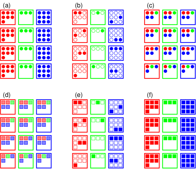
Figure 1: Improved 2D algorithm for processor array of $a=4,b=3$. Circles denote positions, half-toned and filled square denote partial and full forces, respectively. (a) 7, 3 and 9 active particles are found in columns 1, 2 and 3. (b) Each processor in one column decides which particles to handle. (c) Horizontal broadcast of the positions. (d) Force calculation (e) Summation of the partial forces. Completed forces are send back to the original locations. (f) Vertical broadcast of the forces.

Figure 1 illustrates how our new 2D algorithm works. In this example, even if the number of active particles varies widely, the amount of work on each processor is quite well balanced.

4 Optimized force calculation loop

4.1 Functions and the number of operations

In gravitational $N$-body simulations, if parallel efficiency is reasonable, by definition almost all computing time is spent to calculate the gravitational force from one particle to another. With the Hermite integration scheme, what we need to calculate is the acceleration, its time derivative, and the potential, given by

$$\mathbf{a}_{i} = \sum_{j}{m_{j}{\bf r}_{ij}\over(r_{ij}^{2}+\varepsilon^{2})^{3/2}}$$ (1)

$${\bf j}_{i} = {{\bf{\dot{a}}}_{i}}\ =\ \sum_{j}m_{j}\left[{{\bf v}_{ij}\over(r_{ij}^{2}+\varepsilon^{2})^{3/2}}-{3({\bf v}_{ij}\cdot{\bf r}_{ij}){\bf r}_{ij}\over(r_{ij}^{2}+\varepsilon^{2})^{5/2}}\right]$$ (2)

$$\phi_{i} = -\sum_{j}{m_{j}\over(r_{ij}^{2}+\varepsilon^{2})^{1/2}}$$ (3)

where $\mathbf{a}_{i}$ and $\phi_{i}$ are the gravitational acceleration and the potential of particle $i$, the jerk ${\bf j}_{i}$ is the time derivative of the acceleration used for the Hermite integration [16], and ${\bf r}_{i}$, ${\bf v}_{i}$, and $m_{i}$ are the position, velocity and mass of particle $i$, ${\bf r}_{ij}={\bf r}_{j}-{\bf r}_{i}$ and ${\bf v}_{ij}={\bf v}_{j}-{\bf v}_{i}$.

The calculation of $\mathbf{a}$ and $\phi$ requires nine multiplications, 10 addition/subtraction operations, one division and one square root calculation. Warren et al. [24] used 38 as the total number of floating point operations for this pairwise force calculation, and that number has been used by number of researchers. So we follow that convention.

In addition, it requires 11 multiplications and 11 addition/subtraction operations to calculate ${\bf j}$. Thus, the total number of floating-point operations per inner force loop for the Hermite scheme is 60[21].

4.2 Performance tuning

The full details of the optimization we applied is described in [21]. The basic idea is to take full advantage of new functionalities of SSE and SSE2 instructions, without sacrificing the accuracy. The SSE2 instruction set offers the register-based instructions which is easier to optimize than the stack-based x87 instruction set. It also gives SIMD operations for two double-precision words. The SSE instruction set gives SIMD operation on four single-precision words. In addition, it gives fast approximation for inverse square root, which is extremely useful for gravitational force calculation. Our optimized force calculation function uses double-precision SSE2 instructions for the first subtraction of positions and final accumulation of the calculated force, but use SSE single-precision instructions for other operations. Also, fast approximate inverse square root and one Newton-Raphson iteration is used to calculate the inverse square root.

On AMD K8 (Athlon 64 or Opteron) processors, our force loop calculates four gravitational interactions in 120 CPU cycles. In other words, it effectively performs 240 floating-point operations in 120 cycles. The peak performance we can achieve for the force calculation on a single core with 2.2 GHz clock speed is thus 4.4 Gflops. This number happens to be exactly the same as the theoretical peak performance of K8 processors for double-precision operations.

We used an Cray XD1 with 400 2.2GHz dual-core Opteron processors. Therefore, the peak speed we can achieve for the force calculation on single chip is 8.8 Gflops and that for the entire machine is 3.52 Tflops.

5 Simulation of star cluster evolution

In this section, we report the performance of a simulation of the thermal evolution of a star cluster using the parallel individual timestep code we developed.

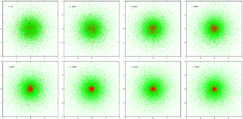
Figure 2: The evolution of the star cluster. The light particles are plotted in green and the heavy particles are plotted in red.

Figure 3: The core density (top) and the core radius (bottom) for $N$-body unit time.

5.1 Model

The problem we study here is the evolution of a two-component star cluster. There have been some works on this kind of system using orbit-averaged Fokker-Plank models[10], but very few works using $N$-body simulation.

We constructed an initial model in the dynamical equilibrium. It is a Plummer model in the Heggie unit [8]. We assign 10% of the total mass to ”heavy” particles, which are 5 times more massive than ”light” particles. Thus, initial model contains 64111 light particles and 1425 massive particles. We used a softened gravitational potential with softening parameter $\varepsilon=4/N$.

5.2 Result

Fig. 2 illustrates the evolution of the mass segregation. The heavy particles lose energy and sink toward the center of the system. Fig. 3 shows the time evolution of the size and mass density of the core calculated using the method described in [4]. We can see that the core shrinks and the evolution becomes faster as the core becomes smaller. We are currently making detailed comparison between $N$-body result and FP calculation result.

5.3 Performance

The total calculation time was 26.4 hours and the total number of timesteps was $4.93\times 10^{10}$, the total number of floating-point operations was $1.94\times 10^{17}$ and the average performance was 2.03 Tflops.

Table 1 gives the breakdown of the calculation time for the period of $1046<t\leq 1047$ (simulation time). Average time per blockstep is around 700 $\mu$s. As we described in the previous section, four complex MPI operations are performed in single blockstep. The fact that the communication took fairly small time is due to the very good performance of MPI library and communication hardware of Cray XD1.

Even with this high-performance MPI library of Cray XD1, without our 2D algorithm, the communication time would increase by at least a factor of 20, and performance would drop to less than 500 Gflops.

Performance	2.37 Gflops
Wall-clock time	54.7 s
Total number of timesteps	$3.26\times 10^{7}$
Total number of block timesteps	$8.07\times 10^{4}$
Avg. calculation time per blockstep	490 $\mu$s
Avg. communication time per blockstep	179 $\mu$s
Avg. $N_{b}$	404

Table 1: Breakdown of the calculation time.

5.4 Scalability

Fig. 4 shows the performance of our parallel $N$-body code on a Cray XD1 with up to 800 (400 dual-core) processors, for $N$=16K and 64K. Multiple symbols for the same values of $N$ and $p$ are results for different processor geometries. In the case of $N$=64k, parallel efficiency is better than 80% for up to 512 processors. Even for 16k particles, efficiency is better than 70% for up to 256 processors, and we achieved the performance of almost one Tflops for 16k particles with 512 processors.

To put our performance result into perspective, we summarize some of the previous works. Dorband et al.[5] obtained around 6 Gflops for $N=16{\rm k}$ on a 128-processor Cray T3E-600. This is around 8% of the theoretical peak of the machine. The best number so far reported on GRAPE-6[19] for $N=16{\rm k}$ is around 130 Gflops, which is 13% of the theoretical peak. We achieved 60% of the theoretical peak of a 256-processor machine for the same number of particles.

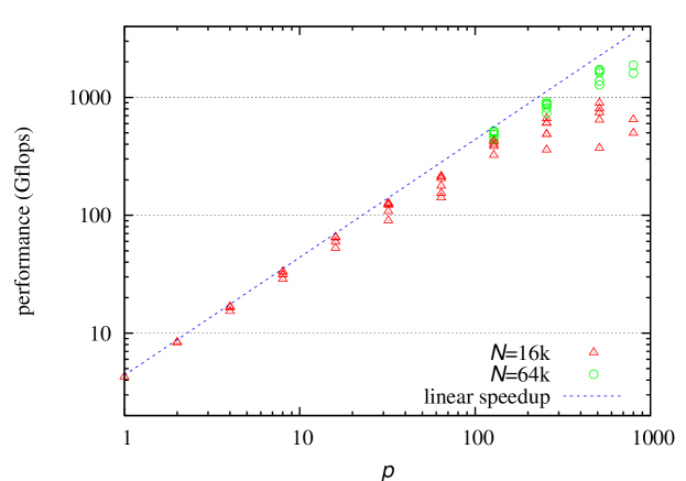
Figure 4: Performance in Gflops as the function of number of processors for $N$=16k (triangle) and $N$=64k (circle). The dotted line indicates the ideal linear speedup.

6 Summary

We developed a new highly scalable parallel algorithm for direct $N$-body simulation with individual (block) timestep integration method. We implemented this new algorithm on a Cray XD1 and achieved quite good performance scaling for up to 800 processors (the largest existing configuration of Cray XD1), for small number of particles such as 16k or 64k. Parallel efficiency better than 80% is obtained for 512 processors, and sustained speed of 2.03 Tflops is achieved for a long calculation on 800 processors.

For the first time, we demonstrated that a modern MPP with $\sim 1000$ processors can be used for astrophysical $N$-body simulations with less than $10^{5}$ particles. This capability to achieve high efficiency for small $N$ is quite important, since the total calculation cost scales as $O(N^{3.3})$ and $N=10^{5}$ is the practical limit of the number of particles we can handle with the effective speed of several Tflops.

We thank Atsushi Kawai and Toshiyuki Fukushige of K&F Computing Research for their stimulating discussions. We are grateful to Hideki Matsumoto of SONY and staffs of Cray Japan for valuable technical supports on the use of the XD1 system. K.N. thanks Shigeo Mitsunari at u10 Networks for discussions on speeding-up of the calculations with assembly-language programming.

References

- [1]
- [2] Aarseth, S. J. 1963, Monthly Notices Roy. Astron. Soc., 126, 223
- [3] Aarseth, S. J. 1985, in Multiple Time Scales, ed. Brackbill and Cohen (Academic Press, New York), p. 377
- [4] Casertano, S., & Hut, P. 1985, ApJ, 298, 80
- [5] Dorband, E. N., Hemsendorf, M. & Merritt, D. 2003, J. Comp. Phys., 185, 484
- [6] Fukushige, T, Makino, J. & Kawai, A. 2005, PASJ, 57, 1009
- [7] Gualandris, A., Portigies Zwart, S. & Tirado-Romos, A. 2004, submitted to IEEE Transactions on Parallel and Distributed Systems (astro-ph/0412206)
- [8] Heggie, D. C. & Mathieu, R. D. 1986, in The Use of Supercomputer in Stellar Dynamics, ed. P. Hut & S. McMillan (New York: Springer), 233
- [9] Hillis, W.D., Barnes, J., Nature, 1987, 326, 27
- [10] Inagaki, S., Wiyanto, P., 1984, PASJ, 36,391
- [11] Kokubo, E., Makino, J., & Ida, S. 1999, AAS/Division for Planetary Sciences Meeting Abstracts, 31,
- [12] Kokubo, E., & Ida, S. 2002, ApJ, 581, 666
- [13] Lippert, T., Ritzenhöfer, G., Glässner, U, Hoeber, H., Seyfried, A. & Schilling, K. 1998 International Journal of Modern Physics C, 7, 485
- [14] Makino, J. 1991a, ApJ, 369, 200
- [15] Makino, J. 1991b, PASJ, 43, 859
- [16] Makino, J. & Aarseth, S. J. 1992, PASJ, 44, 141
- [17] Makino, J. & Fukushige, T. 2001, In The SC2001 Proceedings, CD–ROM. Los Alamitos, IEEE Comp. Soc.
- [18] Makino, J. 2002, New Astronomy, 7, 373
- [19] Makino, J., Fukushige, T., Koga, M., & Namura, K. 2003, PASJ, 55, 1163
- [20] McMillan, S. L. W. 1986, in The Use of Supercomputer in Stellar Dynamics, ed. P. Hut & S. McMillan (New York: Springer), 156
- [21] Nitadori, K., Makino, J. & Hut, P. 2006, New Astronomy, submitted (astro-ph/0511062)
- [22] Springel, V., et al. 2005b, Nat, 435, 629
- [23] Taiji, M. 1998, Highlights of Astronomy, 11, 600
- [24] M. S. Warren, J. K. Salmon, D. J. Becker, M. P. Goda, T. Sterling, and G. S. Winckelmans, in Proceedings of Supercomputing ’97, IEEE Computer Society Press, Los Alamitos, 1997.
- [25]