Using Galaxy Two-point Correlation Functions to Determine the Redshift Distributions of Galaxies Binned by Photometric Redshift

Abstract

We investigate how well the redshift distributions of galaxies sorted into photometric redshift bins can be determined from the galaxy angular two-point correlation functions. We find that the uncertainty in the reconstructed redshift distributions depends critically on the number of parameters used in each redshift bin and the range of angular scales used, but not on the number of photometric redshift bins. Using six parameters for each photometric redshift bin, and restricting ourselves to angular scales over which the galaxy number counts are normally distributed, we find that errors in the reconstructed redshift distributions are large; i.e., they would be the dominant source of uncertainty in cosmological parameters estimated from otherwise ideal weak lensing or baryon acoustic oscillation data. However, either by reducing the number of free parameters in each redshift bin, or by (unjustifiably) applying our Gaussian analysis into the non-Gaussian regime, we find that the correlation functions can be used to reconstruct the redshift distributions with moderate precision; e.g., with mean redshifts determined to $\sim 0.01$. We also find that dividing the galaxies into two spectral types, and thereby doubling the number of redshift distribution parameters, can result in a reduction in the errors in the combined redshift distributions.

To be submitted to ApJ

1 Introduction

There are many different techniques for determining the distance–redshift relation and/or growth–redshift relation motivated by the desire to understand the dark energy. Those that rely on the distances to a relatively small number of objects, such as the Type Ia supernova method (e.g. Riess et al., 1998), can use spectroscopic redshift determinations and thus avoid redshift error as a significant source of uncertainty. However, when the distance (and/or growth) constraints are derived from measurement of very large numbers of objects spectroscopy can be a practical impossibility. In such cases one must rely on “photometric redshifts”; i.e., redshifts estimated from photometry in multiple broad bands (e.g. Loh & Spillar, 1986; Connolly et al., 1995; Sawicki et al., 1997).

The relatively low cost per object of imaging surveys compared to spectroscopic surveys is a great advantage and provides significant motivation for pursuing the technique of estimating photometric redshifts. Imaging surveys can potentially constrain dark energy via a variety of techniques including cluster counting (e.g. Haiman et al., 2001), cosmic shear (e.g. Hu, 2002; Huterer, 2002) and baryon acoustic oscillations (BAO) (e.g. Seo & Eisenstein, 2003; Blake & Glazebrook, 2003; Padmanabhan et al., 2006). It may even be possible for imaging surveys to use Type Ia supernovae, without spectroscopic follow-up, to constrain cosmology (Barris & Tonry, 2004).

But abandoning spectroscopy has its disadavantages too. In general, there is some tolerance of redshift error, but less tolerance for uncertainty about the probability distribution of those errors. The impact of redshift uncertainties on dark energy constraints has been studied for supernovae (Huterer et al., 2004), cluster number counts (Huterer et al., 2004), weak lensing (Bernstein & Jain, 2004; Huterer et al., 2006; Ishak, 2005; Ma et al., 2006) and baryon oscillations (Zhan & Knox, 2005; Zhan, 2006).

All of the studies cited in the above paragraph model the error distribution as Gaussian. However, photometric redshift error distributions, due to spectral-type/redshift degeneracies, often have bimodal distributions, with one smaller peak separated from a larger peak by $\Delta z$ of order unity (e.g. Benítez, 2000; Fernández-Soto et al., 2001, 2002). Thus a fraction of galaxies have photometric redshifts that are ‘catastrophically’ wrong. Here we study how well the coarse properties of the true redshift distribution of galaxies in a given photometric redshift bin can be reconstructed from galaxy two-point correlation functions.

The idea is that catastrophic photometric redshift (“photo-z”) errors introduce additional correlations between galaxies in different redshift bins. In general, such errors will alter both the amplitude and shape of the binned angular correlation functions. Measurements of the correlation functions over a range of angular scales would thus provide valuable information to unravel the effects of large photo-z errors.

We emphasize that we are not attempting a forecast of the photo-z errors achievable given all possible information. In particular, we neglect information from spectroscopic calibration of the photo-z error distribution. Spectroscopy, possibly combined with a “super” photometric (12 or more bands) photo-z training set will play a critical role. In this sense our forecasts here are highly conservative. Further, the catastrophic errors are likely to be avoided by use of luminosity function and surface brightness priors. For recent results on spectroscopic calibration of photo-z measurements for weak lensing, see Ilbert et al. (2006).

The outline of this paper is as follows. In § 2 we describe our model for the photo-z errors, the Fisher matrix we use to constrain the parameters of this model, and our model for the galaxy angular power spectra. We present our results in § 3, including the details of our fiducial model and its impact on the resulting Fisher matrix constraints. We discuss some implications of our results in § 4 and draw conclusions on the feasibility of constraining photo-z errors with galaxy angular correlation functions.

2 Method

In this section, we first introduce our model for the catastrophic photo-z errors, and then describe the Fisher matrix formalism (Jungman et al., 1996; Tegmark et al., 1997) that we use to forecast how well the parameters of this error model can be constrained from observations of the galaxy angular correlation function, binned in redshift. We restrict ourselves to forecasting here and leave for later work the development of a practical algorithm for constraining the photo-z errors in a galaxy survey.

2.1 Model for catastrophic photo-z errors

To focus on the gross mislabeling of galaxy redshifts introduced by catastrophic photo-z errors, we bin the galaxy distribution in redshift and model the errors as a linear mixing of the values of the galaxy number density in each bin. In terms of this model, our goal is then to constrain the number of galaxies from each true-z bin that contribute to the observed number in a given photo-z bin.

We assign the same numerical values for redshift intervals to photo-z bins and true-z bins. The parameters of our error model are then defined as :

$\bar{N}^{a}_{i\alpha}\equiv$ mean number of galaxies per steradian of spectral-type $a$ in photo-z bin $i$ that come from true-z bin $\alpha$.

By considering only the mean number of galaxies mixing between photo-z bins, we are ignoring possible angular fluctuations in the mixing. We expect this to be a good approximation on scales large enough for the fractions of different galaxy types to be uniform, and in the limit of homogeneous noise. The separate index for galaxy sub-populations is to allow for the possibility of different photo-z errors for different galaxy spectral types. However, for most of our results we ignore any information about galaxy types and consider just the parameters $\bar{N}_{i\alpha}\equiv\sum_{a}\bar{N}^{a}_{i\alpha}$ of the entire sample of galaxies.

Using these parameters, we construct the redshift distribution of galaxies in photo-z bin $i$,

$$\frac{dN_{i}^{a}}{dz\,d\Omega}(z,\boldsymbol{\theta})=\sum_{\alpha}\bar{N}^{a}_{i\alpha}\left(\frac{1}{\bar{N}^{a}_{\alpha}}\,\frac{dN^{a}}{dz\,d\Omega}(z,\boldsymbol{\theta})\,\psi_{\alpha}(z)\right)$$ (1)

where $dN^{a}/dzd\Omega$ is the number of galaxies of spectral-type $a$ in redshift interval $dz$ and angular interval $d\Omega$, $\psi_{\alpha}(z)$ is a top-hat window function defining the true-z bin $\alpha$, and

$$\bar{N}^{a}_{\alpha}=\frac{1}{\Omega}\int d\Omega\,\int_{0}^{\infty}dz\,\frac{dN^{a}}{dz\,d\Omega}(z,\boldsymbol{\theta})\,\psi_{\alpha}(z)$$ (2)

is the mean number of galaxies (per steradian) in true-z bin $\alpha$.

Because we are binning in redshift, our model cannot tell us anything about the shape of the redshift distribution within each bin (given by the term in parentheses in eq. 1). We therefore assume that this is known. However, the normalization of the redshift distribution in each bin is determined by the parameters $N^{a}_{i\alpha}$.

If we integrate eq. 1 over redshift, we get an expression for the total number of galaxies (per steradian) in each photo-z bin,

$$N^{a}_{i}(\boldsymbol{\theta})=\sum_{\alpha}\frac{\bar{N}^{a}_{i\alpha}}{\bar{N}_{\alpha}^{a}}\,N^{a}_{\alpha}(\boldsymbol{\theta})$$ (3)

We take the set of $N^{a}_{i}(\boldsymbol{\theta})$ as our data set that we use to constrain the mean parameters $\bar{N}^{a}_{i\alpha}$.

2.2 Fisher matrix

Rephrased in more abstract terms, our problem is to figure out how well a set of parameters $\{a_{p}\}$ can be constrained from a data set $\{N^{a}_{i}\}$, through the influence of $a_{p}$ on the statistical properties of the data.

On large scales, the values of $N^{a}_{i}$ are Gaussian distributed and their statistical properties are completely described by the mean, $\bar{N}^{a}_{i}$, and covariance, $w^{ab}_{ij}(\theta,a_{p})$. However, on small scales, where nonlinear clustering becomes important, the galaxy number density becomes significantly non-Gaussian and higher-order correlations are required to completely describe the statistics of the density field. To avoid the complexities of non-Gaussianity, we limit ourselves to a range in $\theta$ where the data is Gaussian to a good approximation (see section 3.1 for details). Note, however, that there is more information in the data in smaller scales than we are considering here, which could improve the parameter constraints beyond those shown below.

For Gaussian data, the Fisher matrix is given by (Tegmark et al., 1997),

$$F_{pp^{\prime}}=\frac{\partial\mathbf{\bar{N}}^{T}}{\partial a_{p}}\mathbf{w}^{-1}\frac{\partial\mathbf{\bar{N}}}{\partial a_{p^{\prime}}}+\frac{1}{2}\,\text{tr}\left(\frac{\partial\mathbf{w}}{\partial a_{p}}\mathbf{w}^{-1}\frac{\partial\mathbf{w}}{\partial a_{p^{\prime}}}\mathbf{w}^{-1}\right)$$ (4)

where $\mathbf{\bar{N}}$ is the mean of the data and $\mathbf{w}$ is the covariance matrix of the data, defined by,

$$\mathbf{N}=\mathbf{\bar{N}}+\delta\mathbf{N},$$ (5)

with $\mathbf{N}\equiv\{N_{i}^{a}\}$, and

$$\mathbf{w}=\left<\delta\mathbf{N}\,\delta\mathbf{N}^{T}\right>$$ (6)

so that $\mathbf{w}=\left\{w^{ab}_{ij}(\theta,a_{p})\right\}$. In the quadratic approximation to the likelihood, the inverse Fisher matrix is then equal to the covariance of the parameters $a_{p}$.

In this paper, we consider two parameter sets for $\{a_{p}\}$. First, we calculate the Fisher matrix for the parameters $\{\bar{N}^{a}_{i\alpha}\}$. We then add the linear galaxy bias with respect to the dark matter in each redshift bin ($\{b^{a}_{\alpha}\}$) and the amplitude of the power spectrum at $z=0$ (which is degenerate with the galaxy bias at $z=0$) as additional parameters.

The expression for the Fisher matrix in eq. 4 simplifies considerably when we Fourier transform over the variable $\theta$. In this case, the covariance matrix becomes block-diagonal (with one block for each value of the conjugate variable $\ell$) due to isotropy. The second term in eq. 4 then becomes,

$$F^{(2)}_{pp^{\prime}}=\frac{1}{2}\,f_{\text{sky}}\,\sum_{\begin{subarray}{c}\ell\\ (ai)(ai)^{\prime}\\ (bj)(bj^{\prime})\end{subarray}}(2\ell+1)\\ \times\left[\frac{\partial\,C_{(ai)(ai)^{\prime}}}{\partial a_{p}}\left(\mathbf{C}^{-1}\right)_{(ai)^{\prime}(bj)^{\prime}}\frac{\partial\,C_{(bj)^{\prime}(bj)}}{\partial a_{p^{\prime}}}\left(\mathbf{C}^{-1}\right)_{(bj)(ai)}\right],$$ (7)

where $f_{\text{sky}}\,$ is the fractional angular area of the sky covered by the survey, $C_{(ai)(bj)}(\ell)$ is the Fourier transform of $w^{ab}_{ij}(\theta)$ and we have written out the matrix multiplications explicitly.

When we Fourier transform the first term in eq. 4, only the monopole ($\ell=0$) contributes to the mean so that,

$$F^{(1)}_{pp^{\prime}}=\sum_{(ai),(bj)}\frac{\partial\bar{N}^{a}_{i}}{\partial a_{p}}\left(\mathbf{C}^{-1}(\ell=0)\right)_{(ai)(bj)}\frac{\partial\bar{N}^{b}_{j}}{\partial a_{p^{\prime}}}$$ (8)

This term tells us what information the mean of the data contributes to the parameter constraints. Because $\mathbf{\bar{N}}$ does not depend on the galaxy bias, eq. 8 is nonzero only for the parameters $\{\bar{N}^{a}_{i\alpha}\}$.

While formally the cosmological monopole of the power spectrum cannot be determined (because of unknown contributions from super-horizon-sized modes), for a survey that covers only a fraction of the sky, this term will be aliased and will contain contributions from the power spectrum at small (but nonzero) $\ell$. We therefore define an “effective” monopole variance,

$$C_{(ai)(bj)}(\ell=0)\equiv\delta^{K}_{(ai)(bj)}\left(\sigma^{0}_{(ai)}\right)^{2}$$ (9)

From the predicted amplitude of the angular power spectrum at small $\ell$ we set $\sigma^{0}_{(ai)}=10^{-3}\times\bar{N}_{i}^{a}$. We consider this a conservative upper bound.

To avoid confusion in the strict interpretation of this term, we point out that it is identical in form to adding extra Fisher information from an independent measurement of $\mathbf{\bar{N}}$.

Note that, in our notation, Ma et al. (2006) and Zhan (2006) have omitted the term in eq. 8 and instead fixed $\bar{N}_{\alpha}\left(=\sum_{i}\bar{N}_{i\alpha}\right)$. By letting $\bar{N}_{\alpha}$ vary freely, we are assuming no prior knowledge of the true redshift distribution. And by including the term in eq. 8, we are taking into account the fact that the mean number of galaxies in each photo-z bin can be determined from the data. Huterer et al. (2006) and Zhan & Knox (2005) use a method more similar to ours in this respect; i.e., they fix the total number of galaxies in each photometric redshift bin and allow $\bar{N}_{\alpha}$ to vary. Huterer et al. (2006) find there is very little difference between the two approaches for the case of weak lensing. This may not be the case though for galaxy power spectra.

2.3 Galaxy angular power spectrum with photo-z errors

Using eq. 3, the observed angular power spectrum is related to the “true” angular power spectrum (i.e. without photo-z errors) by,

$$C_{(ai)(bj)}(\ell)=\sum_{\alpha\alpha^{\prime}}\,\bar{N}^{a}_{i\alpha}\bar{N}^{b}_{j\alpha^{\prime}}\,P^{ab}_{\alpha\alpha^{\prime}}(\ell),$$ (10)

where bars denote quantities averaged over a redshift bin and $P_{\alpha\alpha^{\prime}}^{ab}(\ell)$ is the power spectrum of the normalized density fluctuations $\delta N^{a}_{\alpha}/\bar{N}^{a}_{\alpha}$ (while $C_{(ai)(bj)}(\ell)$ is the power spectrum of $\delta\bar{N}^{a}_{i}$). We also add shot noise to the model for the observed power spectrum,

$$C^{\text{noise}}_{(ai)(bj)}=\delta^{K}_{(ai)(bj)}\frac{\bar{N}^{a}_{i}\,}{A_{\text{survey}}},$$

where $A_{\text{survey}}$ is the angular area of the survey in square arcminutes and $\delta^{K}$ is the Kronecker delta function. We plot fiducial power spectra given by eq. 10 in fig. 1 along with the variation of the power spectra when one of the parameters $\bar{N}^{a}_{i\alpha}$ is changed by 1-$\sigma$.

We use the halo model to obtain analytic expressions for the linear galaxy bias and nonlinear 3-D galaxy power spectrum as described in the appendix. We then use the Limber approximation (Limber, 1953) to project this into the binned angular galaxy power spectrum,

$$P_{\alpha\beta}^{ab}(\ell)=\delta^{K}_{\alpha\beta}\frac{2\pi^{2}}{\ell^{3}}\int_{0}^{\infty}dz\frac{d\chi}{dz}\left(\Delta^{2}\right)^{ab}_{\alpha\beta}\left(\frac{\ell}{\chi},z\right)\chi\,W_{\alpha}^{a}(\chi)\,W_{\beta}^{b}(\chi)$$ (11)

where $\chi(z)$ is the comoving angular diameter distance as a function of redshift, $\Delta^{2}(k)$ is the 3-D variance of galaxy number density fluctuations per logarithmic interval in $k$, and

$$W_{\alpha}^{a}(\chi)\propto\frac{d\bar{N}^{a}}{d\chi}\psi_{\alpha}(\chi)$$

is the probability distribution for finding a galaxy of type $a$ in $z$-bin $\alpha$ at a comoving distance $\chi$ in the survey, in the absence of photo-z errors, with $\psi_{\alpha}(\chi)$ a top-hat window function for the $z$-bin $\alpha$, as defined in eq. 2, and normalization $\int W_{\alpha}^{a}(\chi)\,d\chi=1$. To simplify the computation, we ignore the redshift evolution of $\Delta^{2}(k,z)$ in eq. 11; evaluating it instead at the mean redshift of the bin.

Note the delta-function in eq. 11 so that our model neglects any intrinsic cross-correlation between redshift bins. For $\ell=50$ (near the peak of the angular power spectrum) and redshift bins with width of 0.5, we have checked that the cross-correlations between bins are less than 1% of the auto-correlations. However, with our fiducial model, the catastrophic photo-z errors induce correlations at the level of $\sim 5$% of the auto-correlation (see fig. 1, left panel). We therefore expect that neglecting intrinsic cross-correlations should not alter our Fisher matrix errors by more than $\sim 1\%$, which is completely unimportant for the conclusions we draw here.

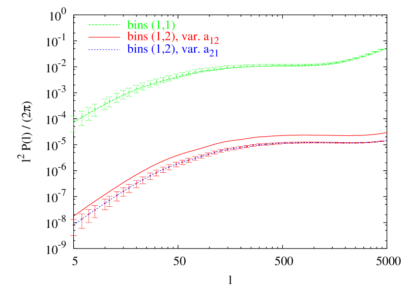
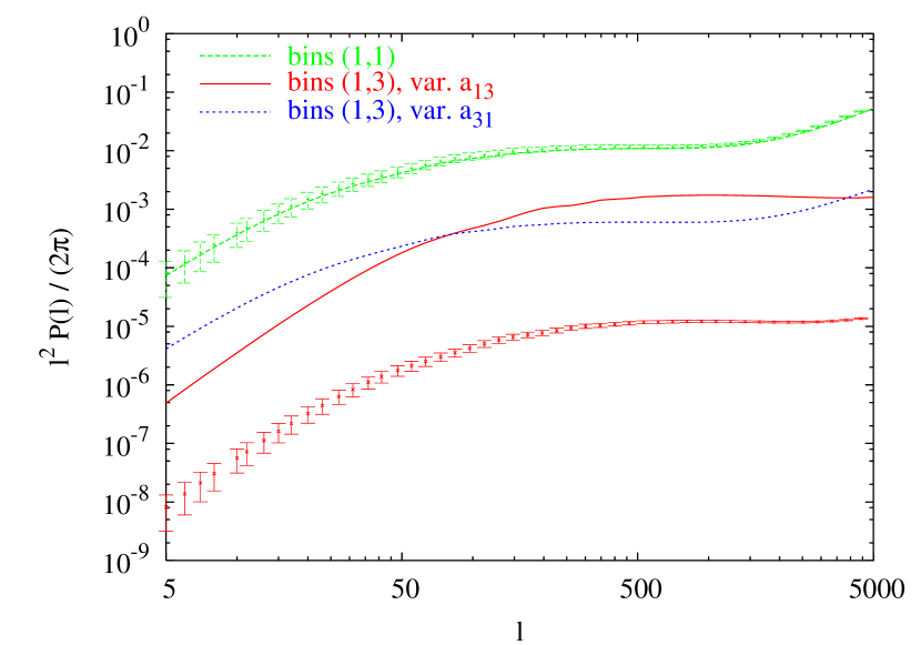
Figure 1: Angular galaxy auto and cross power spectra for photo-z bin 1 in our fiducial model. The points with error bars are the fiducial power spectra, while the lines are 1-$\sigma$ variations of the parameters $a_{12}\equiv\bar{N}_{12}$ or $a_{21}\equiv\bar{N}_{21}$ (left) and $a_{13}\equiv\bar{N}_{13}$ or $a_{31}\equiv\bar{N}_{31}$ (right). For clarity, we have shown only the cross power spectrum that varies the most when the parameters are varied, with the auto power spectra (fiducial points and variation) for reference. The 1-$\sigma$ variations of the parameters are from the Fisher matrix (see fig. 4 below).

An important effect that we have neglected here is magnification of galaxies by weak lensing from intervening large-scale structure (Turner, 1980; Turner et al., 1984). Lensing can induce correlations between different photo-z bins beyond those that would be found in an unlensed model. The amplitude of the weak-lensing induced correlations depends on the luminosity function of the galaxies in the survey, but could be of similar magnitude to the photo-z error induced correlations (Villumsen, 1995). We expect this effect can be calculated with sufficient accuracy that residual uncertainties will not lead to significant confusion with photo-z error induced correlations.

2.4 Galaxy bias parameterization

If we restrict ourselves to linear theory, then the galaxy power spectrum factors into a product of the dark matter power spectrum times a constant (scale-independent but redshift dependent) bias:

$$P^{\text{gal,lin}}_{(a\alpha)(b\beta)}(\ell)=b_{\alpha}^{a}\,b_{\beta}^{b}\,P^{\text{DM,lin}}_{(a\alpha)(b\beta)}(\ell).$$ (12)

At small scales, the bias $b_{\alpha}^{a}$ becomes scale-dependent and this factorization no longer holds. Therefore, when we include the parameters $\{b_{\alpha}^{a}\}$ in our Fisher matrix analysis, we are approximating the galaxy power spectrum with the linear power spectrum. Below, we evaluate the effects of this assumption.

2.5 Galaxy sub-populations

We consider two ways of utilizing the multiband photometric data in a galaxy survey. On the one hand, we imagine assigning photo-z’s to each galaxy and binning them according to their photo-z’s while ignoring any other features of the galaxies. We can then use the number counts in each bin along with our model for the power spectrum to constrain the true redshift distribution of all the galaxies in each bin. On the other hand, we can sort the galaxies according to their spectral (or morphological) type and repeat the analysis (jointly) for each sub-population. From this larger data set, we can then infer constraints on the parameters $\bar{N}_{i\alpha}\equiv\sum_{a}\bar{N}^{a}_{i\alpha}$ for the full galaxy sample by adding the variances of the $\bar{N}^{a}_{i\alpha}$ (including cross-terms). We expect the $\bar{N}^{a}_{i\alpha}$ to be different for each sub-population not only because of different redshift distributions for each galaxy type, but also because of different photo-z error distributions.

While the shot noise increases by dividing the galaxy sample into sub-populations, it may be possible to improve the constraints on the parameters of the total galaxy sample for several reasons. First, we gain knowledge of the mean number density of each sub-group, which contributes to the term in eq. 8. Second, we gain extra information from the cross-correlation between the sub-groups, which is even more helpful if the redshift distribution of one of the types can be well-constrained on its own. In fact, the exposure times and bands for the survey could even be optimized for the best constrained galaxy sub-population. In the limit of exact redshifts of a sub-sample of galaxies, Newman (2006) has shown that cross-correlating with the photo-z sample can place significant constraints on the photo-z errors. Third, a given galaxy sub-group may be more biased than the total galaxy sample and could therefore have equivalent or greater S/N than the total sample even though the noise increases for the sub-samples.

2.6 Mean redshift in each photo-z bin

As discussed in the introduction, we would like to know if the constraints on the photo-z error parameters shown in fig. 4 will be sufficient to enable interesting constraints on dark energy parameters from weak lensing and baryon acoustic oscillation surveys. To properly address this question, we should forecast joint constraints on a suite of cosmological and photo-z parameters with both galaxy and shear data. However, this analysis has already been done for the case of Gaussian photo-z errors (Zhan, 2006) and we choose not to repeat that effort here. Instead, we make contact with previous work by reducing the constraints on the $\bar{N}^{a}_{i\alpha}$ to constraints on the mean redshift in each photo-z bin, defined as,

$$\bar{z}^{a}_{i}\equiv\frac{\int dz\,z\,d\bar{N}^{a}_{i}/dz}{\int dz\,d\bar{N}^{a}_{i}/dz}.$$ (13)

The errors on $\bar{z}_{i}^{a}$ are extracted from the inverse Fisher matrix,

$$\left(F^{-1}_{\bar{z}}\right)_{(ai)(bj)}=\sum_{(ck\beta),(ck\beta)^{\prime}}\frac{\partial\bar{z}^{a}_{i}}{\partial\bar{N}^{c}_{k\beta}}\,\frac{\partial\bar{z}^{b}_{j}}{\partial\bar{N}^{c^{\prime}}_{k^{\prime}\beta^{\prime}}}\,\left(F^{-1}_{\bar{N}}\right)_{(ck\beta)(ck\beta)^{\prime}}$$ (14)

where $F_{\bar{N}}$ is the Fisher matrix in eq. 4.

It has been shown in Huterer et al. (2006); Ma et al. (2006); Zhan & Knox (2005); Zhan (2006) that useful dark energy constraints require the error on the mean redshift in each photo-z bin to be constrained to $\sim 0.003$ near $z\simeq 1$, and increasing rapidly towards higher redshift. We therefore use 0.003 as a benchmark for assessing our results.

3 Results

In this section, we first describe a simple fiducial model for the galaxy survey and photo-z errors, and then show the forecasted constraints from the Fisher matrix in eq. 7. We then study how our results depend on the fiducial model in order to draw conclusions independent of the many assumptions in our model.

3.1 Fiducial model

We choose our fiducial model to mimic the LSST. Throughout, we consider a survey covering 20,000 sq. deg. and bin the galaxies in photo-z over the range 0 to 3. Our fiducial cosmological parameters are $\Omega_{m}=0.24$, $\Omega_{b}h^{2}=0.022$, $\Omega_{\Lambda}=0.76$, $h=0.72$, and $\sigma_{8}=0.74$.

To ensure that our assumption of Gaussianity in eq. 4 is reasonable, we limit the $\ell$ range in eq. 10 by adding large noise to each element of $P_{(ai)(bj)}(\ell)$ with $\ell>\ell_{\text{max}}(z)$, where $\ell_{\text{max}}(z)\equiv\chi(z)\,k_{\text{max}}(z)$ and $\Delta^{2}_{\text{DM}}(k_{\text{max}},z)=0.4$. We also set a lower bound on $\ell$ to justify our use of the Limber approximation for the angular power spectrum in eq. 11. The Limber approximation relies on the observation that, when projecting the 3-D power spectrum into 2 dimensions, the dominant contribution is from those Fourier modes that do not oscillate significantly along the line of sight. We can quantify this statement by considering only modes with line-of-sight component of the wavevector $k_{3}<2\pi/\Delta\chi(z)$, where $\Delta\chi(z)$ is the comoving width of the $z$-bin under consideration. The Limber approximation also requires $\ell\gg k_{3}\chi(z)$. Putting these together, we set $\ell_{\text{min}}(z)\equiv 4\pi\chi(z)/\Delta\chi$ (with an arbitrary factor of 2 inserted just to be conservative).

Table 1: Multipole range for the galaxy power spectrum as a function of redshift

$z$ range	$\ell_{\text{min}}(z)$	$\ell_{\text{max}}(z)$
0.0 – 0.5	7	114
0.5 – 1.0	23	458
1.0 – 1.5	45	1018
1.5 – 2.0	71	1875
2.0 – 2.5	103	3195
2.5 – 3.0	140	5186

In table 1, we show the values of $\ell_{\text{max}}$, as a function of redshift in our fiducial model for 6 $z$-bins over the range $0\leq z\leq 3$. We evaluate both $\ell_{\text{min}}$ and $\ell_{\text{max}}$ at the centers of the photo-z bins.

We use the redshift distribution from Song & Knox (2003) (which is based on Subaru observations with limiting magnitude in $R$ of 26),

$$\frac{d\bar{N}}{dz\,d\Omega}(z)=\bar{N}_{\text{tot}}\,\exp\left[-\left(\frac{z}{1.2}\right)^{1.2}\right]\times\begin{cases}z^{1.3}&z<1\\ z^{1.1}&z>1\end{cases}$$ (15)

with the normalization, $\bar{N}_{\text{tot}}$ set by $\int dz\,d\bar{N}/dz\,d\Omega=65$ per sq. arcmin.

When considering galaxy sub-populations, we consider two spectral types that we label “red” and “blue,” roughly depending on the absence or presence of active star formation. In the absence of a well-motivated model, we generated several redshift distributions for the red and blue sub-populations in an ad-hoc fashion, and compared the results between them. We require only that the redshift distributions sum to give eq. 15 and that the blue distribution dominate at large redshifts ($z\gtrsim 1$).

For the red and blue galaxy sub-populations, we set

$$\frac{d\bar{N}^{\text{red}}}{dz\,d\Omega}=R\,\bar{N}_{\text{tot}}\,z^{1.4}\,\exp\left[-r_{1}z^{r_{2}}\right]$$ (16)

and

$$\frac{d\bar{N}^{\text{blue}}}{dz\,d\Omega}=\frac{d\bar{N}}{dz\,d\Omega}-\frac{d\bar{N}^{\text{red}}}{dz\,d\Omega}$$

with $R=0.8$, $r_{1}=1.3$, $r_{2}=1.4$. These fiducial redshift distributions are shown in fig. 2.

Figure 2: Fiducial redshift distributions for the “red” and “blue” galaxy sub-populations (eq. 16) and the total galaxy sample (“total,” eq. 15).

Our fiducial model for $\bar{N}^{a}_{i\alpha}$ is based on the estimated photo-z’s for a simulated random sample of 100,000 galaxies over redshifts from 0 to 4 with colors assigned by filtering spectra from a sample of 10 redshift-evolved spectral energy distributions (SEDs). The simulation assumed photometric data was available in 6 filters ($ugrizy$), modelled after the LSST, with the data limited in the $i$-band at $i<25$ and an S/N of 10-15 at the depth of the survey. The depth of the simulation is what one would achieve after about 400 visits per filter. This is just a fiducial approach as the errors can be optimized by weighting the exposure times in each band separately. The photo-z of each galaxy was estimated by matching the galaxy colors with a SED template library. No priors on the luminosity function or surface brightness were used, which can significantly improve the photo-z estimates in some cases. In this regard, our fiducial model is therefore a worst-case scenario.

To model the errors for the galaxy sub-populations, we divided the templates for the simulated galaxy SEDs into 2 groups based on the presence or absence of strong emission lines.

The fiducial parameters, $\bar{N}^{a}_{i\alpha}$, are constructed by first creating the matrix, $E^{a}_{i\alpha}\equiv\bar{N}^{a}_{i\alpha}/\bar{N}^{a}_{\alpha}$, by binning the photo-z vs. $z$ plane and normalizing so that $\sum_{i}E^{a}_{i\alpha}=1$ (for each $a$ and $\alpha$). This normalization conserves the total number of galaxies in the survey. We then use the fiducial redshift distribution in eq. 15 to create $\bar{N}^{a}_{\alpha}$ according to eq. 2 and multiply with $E^{a}_{i\alpha}$ to get the parameters $\bar{N}^{a}_{i\alpha}$. An example of our fiducial model for the $\bar{N}^{a}_{i\alpha}$ is plotted in fig. 3.

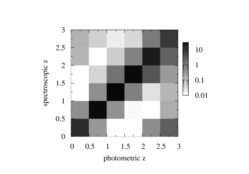
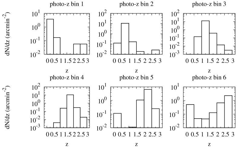
Figure 3: The fiducial redshift distribution with catastrophic photo-z errors: $\bar{N}^{a}_{i\alpha}$ (for the “LSST” model – see text). The two plots show the same parameters in different perspectives. On the left, is the number density, $\bar{N}^{a}_{i\alpha}$, as a function of redshift (indexed by $i$ = photometric $z$ and $\alpha$ = spectroscopic $z$). On the right, each window shows a different photo-z bin index, $i$, while each bar in a given window shows a different spectroscopic index, $\alpha$, for the given $i$. For example, the bar between $z=0.5$ and $z=1$ in the window for “photo-z bin 1” is the number density of galaxies with spectroscopic redshifts in the range $0.5<z<1$ that have been given photometric redshifts in the range $0<z<0.5$.

3.2 Parameter constraints

Our main results are in fig. 4, which shows the Fisher constraints on the parameters $\bar{N}_{i\alpha}$ assuming a 10% prior on the galaxy bias and 100% prior on the $\bar{N}^{a}_{i\alpha}$. The model for the open squares includes the “red” and “blue” galaxy sub-populations, while the model for the filled squares ignores this information.

Figure 4: Forecasted constraints for the parameters $\bar{N}_{i\alpha}$ divided by the fiducial $\bar{N}_{i}$ in each photo-z bin, i.e. the error on the fraction of outliers within each photo-z bin. The filled squares are the fractional constraints when no galaxy sub-populations are considered, while the open squares are the constraints when the galaxy sample is divided into “red” and “blue” spectral types. For the open squares, the parameters for the “red” and “blue” sub-populations ($\bar{N}^{a}_{i\alpha}$) were constrained first, and then these constraints were combined to produce the constraints on $\bar{N}_{i\alpha}$ shown here (by summing over the index $a$ in the inverse Fisher matrix components). A 10% prior on the galaxy bias and a 100% prior on the $\bar{N}^{a}_{i\alpha}$ were imposed. The fiducial model assumed “LSST” photo-z errors (see text) and sky coverage of 20,000 sq. deg.

In the column 2 of table 2, we show the constraints on the mean redshift in each photo-z bin (eq. 14) implied by the constraints on the $\bar{N}^{a}_{i\alpha}$ without galaxy sub-populations (filled squares in fig. 4). These are two orders of magnitude larger than the “benchmark” value (described in section 2.6) needed for constraining dark energy parameters. In the following subsections, we discuss three ways that the constraints on $\bar{z}_{i}$ could possibly be improved.

Table 2: Constraints on the mean redshift of each photo-z bin

$z$ range	$\sigma_{\text{LSST}}$	$\sigma_{\text{sub}}$	$\sigma_{\text{Gauss}}$	$\sigma_{\ell_{\text{max}}=4000}$
0.0 – 0.5	0.29	0.059	0.0050	0.0030
0.5 – 1.0	0.068	0.041	0.010	0.0050
1.0 – 1.5	0.12	0.036	0.0087	0.0096
1.5 – 2.0	0.16	0.049	0.0091	0.016
2.0 – 2.5	0.23	0.085	0.0079	0.022
2.5 – 3.0	0.28	0.61	0.0047	0.025

3.2.1 Adding galaxy sub-populations

For a wide range of fiducial models, we find that dividing our galaxy sample into “red” and “blue” sub-populations improves the forecasted constraints on the redshift distribution in each photo-z bin, as shown by the open squares in fig. 4 and column 3 of table 2. We also show forecasted constraints on the redshift distributions of the sub-populations in fig. 5. Comparing the errors on the mean redshift in each photo-z bin in table 2, we see that there is a significant improvement over the constraints obtained without using information about galaxy sub-populations, but is still much larger than the “benchmark” for dark energy surveys given in section 2.6

Because our fiducial models for the biases and redshift distributions of the sub-populations (in the absence of photo-z errors) are rather ad-hoc, we have varied the parameters in eqs. 16 and A2 over a range of physically reasonable values and find no change to the qualitative nature of our results. This is discussed more in section 3.3.2.

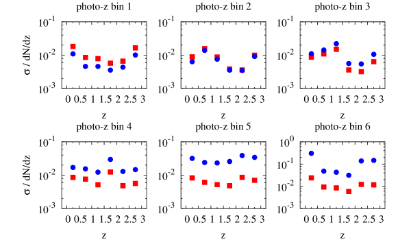
Figure 5: Forecasted fractional constraints on $\bar{N}^{a}_{i\alpha}$ for the “red” (squares) and “blue” (circles) galaxy sub-populations. These constraints take into account the cross-correlation between the red and blue samples. We used a 10% prior on the linear galaxy bias and a 100% prior on the $\bar{N}^{a}_{i\alpha}$.

3.2.2 Sensitivity to parameterization

We show in the left panel of fig. 6 and column 3 of table 2 the forecasted parameter constraints with a fiducial photo-z error model that only allows mixing between adjacent photo-z bins and with the number of photo-z error parameters reduced to only those that can take nonzero values in the fiducial model. The fiducial errors assume a 5% contribution from each of the adjacent bins to a given photo-z bin. This crudely mimics a Gaussian model for the photo-z errors. We have also tightened the prior on the galaxy bias from 10% to 1%. While the constraints on the $\bar{N}^{a}_{i\alpha}$ in the left panel of fig. 6 are moderately improved from the default model in fig. 4, the constraints on $\bar{z}_{i}$ in table 2 improve by nearly two orders of magnitude. This shows that reducing the number of free parameters in each photo-z bin indeed has a large impact on the ability to constrain the redshift distribution in each bin.

3.2.3 Sensitivity to range of angular scales

The forecasted constraints are very sensitive to the maximum $\ell$ used in the galaxy power spectrum (but are rather insensitive to the minimum $\ell$ cutoff). In particular, for the lowest photo-z bin, the maximum cutoff at $\ell=114$ (from table 1) removes some of the baryon features in the power spectrum that can help in diagnosing photo-z errors (Zhan, 2006).

To demonstrate this sensitivity, we show the forecasted constraints when $\ell_{\text{max}}(z)=4000$ for all $z$ in the right panel of fig. 6 and column 5 of table 2. The constraints on the mean redshift in each photo-z bin are two orders of magnitude smaller than those with $\ell_{\text{max}}$ from table 1 (labelled $\sigma_{\text{LSST}}$ in table 2).

Recall that the maximum $\ell$ cutoff is imposed to validate our assumption of Gaussian data (in e.g. eq. 4). Therefore, the constraints presented in this section should be interpreted only up to non-Gaussian corrections, which could be quite large. Our results are an indication that there is much to be gained by developing the appropriate tools for analyzing the non-Gaussian case.

Figure 6: Demonstration of two factors that significantly affect the errors on the mean redshift in each photo-z bin (see table 2). For the filled squares on the left, we have chosen a fiducial photo-z error model that only introduces mixing between adjacent bins and have fixed the parameters that are known to be zero in this model. This roughly mimics a Gaussian photo-z error distribution. For the filled squares on the right, we have replaced the $z$-dependent $\ell$ cutoff from table 1 with a maximum $\ell=4000$ for all the photo-z bins. For reference, the open squares in both plots show the constraints with the default fiducial model without galaxy sub-populations. The left panel assumes a 1% prior on the linear galaxy bias, while right panel assumes a 10% prior.

3.3 Fiducial model dependence

To test the robustness of our conclusions, we recomputed the Fisher matrix in eq. 7 while varying the number of redshift bins, the galaxy bias and halo occupation distribution in the nonlinear power spectrum, and the fiducial model for the photo-z errors.

3.3.1 Redshift distribution

For comparison, we use a second fiducial model for $E^{a}_{i\alpha}$ with 10% of the galaxies in each photo-z bin uniformly distributed over the remaining photo-z bins. This model, though not physically motivated, gives us a reference for determining the sensitivity of the Fisher constraints to the fiducial error model.

We show ratios of the Fisher matrix errors obtained with these two fiducial photo-z error models in fig. 7. For most of the parameters, the different fiducial models lead to differences in the forecasted errors of a factor of $\lesssim 5$. The LSST fiducial model for the photo-z errors is actually well-motivated by our photo-z estimation simulation so any uncertainties in the fiducial model will be much smaller than the changes introduced by this artificial “uniform” error model. We therefore conclude that uncertainties in the fiducial photo-z errors will affect our forecasted constraints by factors of $\lesssim$ a few.

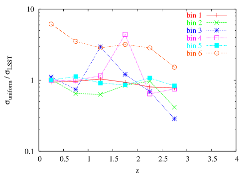
Figure 7: Ratios of forecasted errors for the parameters $\bar{N}_{i\alpha}$ using 2 different fiducial models for the photo-z errors. We first scale the forecasted errors by the fiducial $\bar{N}_{i}$ in each photo-z bin (to obtain fractional errors) and then divide the errors obtained using a uniform distribution of 10% scatter from each photo-z bin by the forecasted errors obtained using a photo-z error model based on the LSST (see text). Each line shows a different photo-z bin (corresponding to the index $i$ in the parameters).

3.3.2 Galaxy bias and nonlinear power spectrum

The results we have shown so far model the galaxy power spectrum using only the linear theory prediction. To make sure that this approximation will not affect the qualitative nature of our results, we compare in fig. 8 the forecasted errors for the photo-z error distribution obtained using the linear theory power spectrum to those obtained with the nonlinear model (see the appendix). We see that our use of the linear power spectrum is a good approximation, which is to be expected given our truncation in $\ell$ described at the beginning of section 3.1.

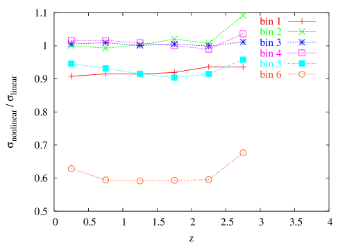
Figure 8: Ratios of forecasted constraints for the parameters $\bar{N}_{i\alpha}$ using the nonlinear power spectrum divided by the constraints using the linear theory power spectrum. The fiducial redshift distribution and photo-z errors are the same in each case. Each line shows a different photo-z bin (corresponding to the index $i$ in the parameters).

The fiducial linear galaxy bias and nonlinear galaxy power spectrum depend on a model for the way that galaxies populate dark matter halos. The details of our fiducial model are explained in the appendix, section A.1, but this model has only been very loosely constrained by observations (Cooray, 2006; Abazajian et al., 2005). Therefore to build confidence in our use of a necessarily ad hoc fiducial model, we compared the parameter constraints from the Fisher matrix when we vary the ad hoc parameters. We find that when the “satellite” galaxy normalization and slope (defined in eq. A2) are varied by 50% and 25% respectively, the changes in the photo-z error parameter constraints are less than 10% and 0.01% for all the redshift bins. This amount of variation will not affect our conclusions.

3.3.3 Number of photo-z bins

We have compared the fractional constraints on the photo-z error parameters when the number of photo-z bins is varied from 2 to 10 and do not find a significant variation. As the number of photo-z bins is increased, there is more information about the photo-z errors from the additional cross-correlations between photo-z bins, but the number of parameters to constrain also increases. So, the fractional constraints we show here for six bins should be representative of the constraints that would be obtained for any moderate number of bins. Note, however, that having the same fractional constraints for a larger number of parameters means we have more information about the photo-z error distribution with photo-z bins. Of course, for a sufficiently large number of photo-z bins, the shot noise will begin to dominate.

4 Discussion and Conclusions

We have shown that the ability to constrain general (i.e. non-Gaussian) photo-z error distributions with galaxy two-point correlation functions depends on the parameterization of the photo-z errors, the range of angular scales probed by the correlation function, and prior knowledge of the galaxy bias.

Binning the galaxy sample in photo-z, we have presented constraints on the binned redshift distribution and mean redshift in each photo-z bin. Parameterizing the redshift distribution by binned values is insensitive to small scatter from photo-z errors, but otherwise assumes no a priori knowledge of the photo-z error distribution. We find that reducing the number of parameters in each photo-z bin can be very helpful, which could be achieved with improved knowledge of the photo-z errors from, e.g., spectroscopically calibrated samples or luminosity function priors.

We have limited our use of the galaxy correlation function to angular scales where the galaxy number density is Gaussian distributed. At low redshifts, this severely limits the amount of data available to constrain the photo-z error parameters. We hypothesize that including information from correlations on non-Gaussian scales could significantly improve the constraints and demonstrate that the constraints on the mean redshift in each photo-z bin do improve by two orders of magnitude with a naive extrapolation of our Gaussian calculation to non-Gaussian scales.

If it is possible to separate the galaxies by spectral type, the constraints on the photo-z errors may improve further by including information from the cross-correlation of the galaxy sub-samples. We have demonstrated this in figs. 4 and 5 by separating our fiducial galaxy sample into “red” and “blue” spectral types. We expect this procedure to be particularly helpful if there exists a well-populated spectral class of galaxies whose photo-z’s can be estimated unusually well.

Our forecasts are limited to parameters of the photo-z error distribution and linear galaxy bias so we cannot make any rigorous conclusions about what kind of dark energy constraints can be achieved in weak lensing and baryon acoustic oscillation surveys with the level of photo-z errors forecasted here. However, we make qualitative comparisons with dark energy forecasts in the literature (Huterer et al., 2006; Ma et al., 2006; Zhan & Knox, 2005; Zhan, 2006) using our constraints on the mean redshift in each photo-z bin given in table 2. In the Gaussian regime, the constraints we forecast of $\sim 0.01$ are factors of a few larger than those desired for upcoming dark energy surveys. However, adding non-Gaussian scales in the correlation function may provide the required constraints. The galaxy correlation properties are quite likely to provide at least a powerful consistency test for the redshift distributions as determined via spectroscopic and/or “super” (12 or more band) calibration subsamples.

A Halo model

The halo model (for a review see Cooray & Sheth, 2002) provides an analytic approximation to the nonlinear three-dimensional galaxy power spectrum using the assumptions that all the dark matter is contained in gravitationally bound “halos” of varying mass and that the number of galaxies populating a given dark matter halo is determined solely by the halo mass and redshift. The model for the number of galaxies in a dark matter halo is often referred to as the “halo occupation distribution” (HOD).

A.1 Fiducial HOD models

Following Hu & Jain (2004), we divide the mean number of galaxies in a dark matter halo of mass $m$ into contributions from a galaxy at the halo’s center ($\bar{N}_{c}$) and satellite galaxies ($\bar{N}_{s}$). The mean number of central galaxies is essentially a unit step function parameterized by a minimum threshold mass, $m_{\text{th}}(z)$, for a halo to host a galaxy. To allow for scatter in the relation between galaxy luminosity and halo mass, the simple step function is modified to,

$$\bar{N}_{c}^{a}(m,z)=\frac{1}{2}\,f^{a}(m,z)\,\operatorname{Erfc}\left(\frac{\log(m_{\text{th}}(z)/m)}{\sqrt{2}\,\sigma}\right),$$ (A1)

where $f^{a}(m,z)$ is the fraction of central galaxies of spectral type $a$. We use eq. 7 in Cooray (2006) as our fiducial model for $f^{a}(m,z)$ and set $\sigma=0.1$.

The mean number of satellite galaxies is modelled as a power law,

$$\bar{N}_{s}(m,z)=\left(\frac{m}{A\,m_{\text{th}}(z)}\right)^{b},$$ (A2)

with the two free parameters $A\sim 30$, $b\sim 1$ (Hu & Jain, 2004).

The threshold mass, $m_{\text{th}}$, is determined by requiring the HOD model to reproduce the fiducial redshift distribution as follows:

$$\frac{d\bar{N}}{dz\,d\Omega}(z) =\chi^{2}(z)\frac{d\chi}{dz}\,\int dm\,n(m,z)\left(\bar{N}_{c}(m,z)+\bar{N}_{s}(m,z)\right)$$

$$\equiv\chi^{2}(z)\frac{d\chi}{dz}\,\bar{n}_{g}(z),$$ (A3)

where $\chi(z)$ is the comoving distance as a function of redshift and $n(m,z)$ is the halo mass function (we use the Sheth-Tormen model for $n(m,z)$ (Sheth & Tormen, 1999)).

A.2 Galaxy power spectrum

The power spectrum of galaxies in the halo model is the sum of two terms:

$$P_{g}(k,z_{1},z_{2})=P_{1h}(k,z_{1},z_{2})+P_{2h}(k,z_{1},z_{2}),$$

where,

$$P_{1h}(k,z_{1},z_{2})\equiv\frac{\delta_{z_{1},z_{2}}}{\bar{n}_{g}^{2}(z_{1})}\int dm\,n(m,z)\\ \times\left(\bar{N}_{s}^{2}(m,z_{1})\,u_{g}^{2}(k|z_{1},m)+2\bar{N}_{c}(m,z_{1})\bar{N}_{s}(m,z_{1})u_{g}(k|z_{1},m)\right)$$

is the contribution to the power from a single halo, and

$$P_{2h}(k,z_{1},z_{2})\equiv P^{\text{lin}}(k,z_{1},z_{2})\,I_{2}(k,z_{1})\,I_{2}(k,z_{2})$$ (A4)

with,

$$I_{2}(k,z)\equiv\frac{1}{\bar{n}_{g}(z)}\int dm\,n(m,z)\,b_{h}(m,z)\\ \times\left(\bar{N}_{c}(m,z)+\bar{N}_{s}(m,z)u_{g}(k|z,m)\right)$$

is the contribution from 2 different halos. Here, $u_{g}(k|z,m)$ is the Fourier transform of the galaxy number density profile (assumed to follow the NFW profile (Navarro et al., 1996)), $b_{h}(m,z)$ is the halo bias (specified in the Sheth-Tormen model along with the mass function) and $\bar{n}_{g}(z)$ is the mean comoving number density of galaxies defined in eq. A.1.

A.3 Linear power spectrum

The linear power spectrum in eq. A4 is the variance per logarithmic interval in $k$, in linear perturbation theory

$$P^{\text{lin}}(k,z_{1},z_{2})\equiv\delta_{H}^{2}(0)\,g(z_{1})\,g(z_{2})\left(\frac{ck}{H_{0}}\right)^{n+3}T^{2}(k)$$

where $\delta_{H}(0)$ is the amplitude at $z=0$, $g(z)$ is the linear growth function, $T(k)$ is the transfer function, and $H_{0}$ is the Hubble constant. We take a fiducial value of $n=1$.

A.4 Linear galaxy bias

The galaxy bias in the halo model is given by,

$$b^{a}\left(z_{\alpha}\right)=\int dm\,n(m,z_{\alpha})\,b_{h}(m,z_{\alpha})\,\frac{\left(\bar{N}^{a}_{c}+\bar{N}^{a}_{s}\right)(m,z_{\alpha})}{\bar{n}_{g}^{a}(z_{\alpha})},$$ (A5)

where the superscript ($a$) labeling different galaxy sub-populations denotes different values of the parameters $A$ and $b$ in eq. A2 and $m_{\text{th}}$.

References

- Abazajian et al. (2005) Abazajian, K., Zheng, Z., Zehavi, I., Weinberg, D. H., Frieman, J. A., Berlind, A. A., Blanton, M. R., Bahcall, N. A., Brinkmann, J., Schneider, D. P., & Tegmark, M. 2005, ApJ, 625, 613
- Barris & Tonry (2004) Barris, B. J. & Tonry, J. L. 2004, ApJ, 613, L21
- Benítez (2000) Benítez, N. 2000, ApJ, 536, 571
- Bernstein & Jain (2004) Bernstein, G. & Jain, B. 2004, ApJ, 600, 17
- Blake & Glazebrook (2003) Blake, C. & Glazebrook, K. 2003, ApJ, 594, 665
- Connolly et al. (1995) Connolly, A. J., Csabai, I., Szalay, A. S., Koo, D. C., Kron, R. G., & Munn, J. A. 1995, AJ, 110, 2655
- Cooray (2006) Cooray, A. 2006, MNRAS, 365, 842
- Cooray & Sheth (2002) Cooray, A. & Sheth, R. 2002, Phys. Rep., 372, 1
- Fernández-Soto et al. (2002) Fernández-Soto, A., Lanzetta, K. M., Chen, H.-W., Levine, B., & Yahata, N. 2002, MNRAS, 330, 889
- Fernández-Soto et al. (2001) Fernández-Soto, A., Lanzetta, K. M., Chen, H.-W., Pascarelle, S. M., & Yahata, N. 2001, ApJS, 135, 41
- Haiman et al. (2001) Haiman, Z., Mohr, J. J., & Holder, G. P. 2001, ApJ, 553, 545
- Hu (2002) Hu, W. 2002, Phys. Rev. D, 66, 83515
- Hu & Jain (2004) Hu, W. & Jain, B. 2004, Phys. Rev. D, 70, 043009
- Huterer (2002) Huterer, D. 2002, Phys. Rev. D, 65, 63001
- Huterer et al. (2004) Huterer, D., Kim, A., Krauss, L. M., & Broderick, T. 2004, ApJ, 615, 595
- Huterer et al. (2006) Huterer, D., Takada, M., Bernstein, G., & Jain, B. 2006, MNRAS, 366, 101
- Ilbert et al. (2006) Ilbert, O., Arnouts, S., McCracken, H. J., Bolzonella, M., Bertin, E., Le Fevre, O., Mellier, Y., Zamorani, G., Pello, R., Iovino, A., Tresse, L., Bottini, D., Garilli, B., Le Brun, V., Maccagni, D., Picat, J. P., Scaramella, R., Scodeggio, M., Vettolani, G., Zanichelli, A., Adami, C., Bardelli, S., Cappi, A., Charlot, S., Ciliegi, P., Contini, T., Cucciati, O., Foucaud, S., Franzetti, P., Gavignaud, I., Guzzo, L., Marano, B., Marinoni, C., Mazure, A., Meneux, B., Merighi, R., Paltani, S., Pollo, A., Pozzetti, L., Radovich, M., Zucca, E., Bondi, M., Bongiorno, A., Busarello, G., De La Torre, S., Gregorini, L., Lamareille, F., Mathez, G., Merluzzi, P., Ripepi, V., Rizzo, D., & Vergani, D. 2006, ArXiv Astrophysics e-prints
- Ishak (2005) Ishak, M. 2005, MNRAS, 363, 469
- Jungman et al. (1996) Jungman, G., Kamionkowski, M., Kosowsky, A., & Spergel, D. N. 1996, Phys. Rev. D, 54, 1332
- Limber (1953) Limber, D. N. 1953, ApJ, 117, 134
- Loh & Spillar (1986) Loh, E. & Spillar, E. 1986, ApJ, 303, 154
- Ma et al. (2006) Ma, Z., Hu, W., & Huterer, D. 2006, ApJ, 636, 21
- Navarro et al. (1996) Navarro, J. F., Frenk, C. S., & White, S. D. M. 1996, ApJ, 462, 563
- Newman (2006) Newman, J. A. 2006, in preparation
- Padmanabhan et al. (2006) Padmanabhan, N., Schlegel, D. J., Seljak, U., Makarov, A., Bahcall, N. A., Blanton, M. R., Brinkmann, J., Eisenstein, D. J., Finkbeiner, D. P., Gunn, J. E., Hogg, D. W., Ivezic, Z., Knapp, G. R., Loveday, J., Lupton, R. H., Nichol, R. C., Schneider, D. P., Strauss, M. A., Tegmark, M., & York, D. G. 2006, ArXiv Astrophysics e-prints
- Riess et al. (1998) Riess, A. G., Filippenko, A. V., Challis, P., Clocchiatti, A., Diercks, A., Garnavich, P. M., Gilliland, R. L., Hogan, C. J., Jha, S., Kirshner, R. P., Leibundgut, B., Phillips, M. M., Reiss, D., Schmidt, B. P., Schommer, R. A., Smith, R. C., Spyromilio, J., Stubbs, C., Suntzeff, N. B., & Tonry, J. 1998, AJ, 116, 1009
- Sawicki et al. (1997) Sawicki, M. J., Lin, H., & Yee, H. K. C. 1997, AJ, 113, 1
- Seo & Eisenstein (2003) Seo, H. & Eisenstein, D. J. 2003, ApJ, 598, 720
- Sheth & Tormen (1999) Sheth, R. K. & Tormen, G. 1999, MNRAS, 308, 119
- Song & Knox (2003) Song, Y. & Knox, L. 2003, ArXiv: astro-ph/0312175
- Tegmark et al. (1997) Tegmark, M., Taylor, A. N., & Heavens, A. F. 1997, ApJ, 480, 22+
- Turner (1980) Turner, E. L. 1980, ApJ, 242, L135
- Turner et al. (1984) Turner, E. L., Ostriker, J. P., & Gott, III, J. R. 1984, ApJ, 284, 1
- Villumsen (1995) Villumsen, J. V. 1995, ArXiv: astro-ph/9512001
- Zhan (2006) Zhan, H. 2006, ArXiv: astro-ph/0605696
- Zhan & Knox (2005) Zhan, H. & Knox, L. 2005, ArXiv: astro-ph/0509260