Solar dynamo models with $\alpha$-effect and turbulent pumping from local 3D convection calculations

Abstract

Results from kinematic solar dynamo models employing $\alpha$-effect and turbulent pumping from local convection calculations are presented. We estimate the magnitude of these effects to be around 2–3 m s^-1, having scaled the local quantities with the convective velocity at the bottom of the convection zone from a solar mixing-length model. Rotation profile of the Sun as obtained from helioseismology is applied in the models; we also investigate the effects of the observed surface shear layer on the dynamo solutions. With these choices of the small- and large-scale velocity fields, we obtain estimate of the ratio of the the two induction effects, $C_{\alpha}/C_{\Omega}\approx 10^{-3}$, which we keep fixed in all models. We also include a one-cell meridional circulation pattern having a magnitude of 10–20 m s^-1 near the surface and 1–2 m s^-1 at the bottom of the convection zone. The model essentially represents a distributed turbulent dynamo, as the $\alpha$-effect is nonzero throughout the convection zone, although it concentrates near the bottom of the convection zone obtaining a maximum around $30\degr$ of latitude. Turbulent pumping of the mean fields is predominantly down- and equatorward. The anisotropies in the turbulent diffusivity are neglected apart from the fact that the diffusivity is significantly reduced in the overshoot region. We find that, when all these effects are included in the model, it is possible to correctly reproduce many features of the solar activity cycle, namely the correct equatorward migration at low latitudes and the polar branch at high latitudes, and the observed negative sign of $B_{r}B_{\phi}$. Although the activity clearly shifts towards the equator in comparison to previous models due to the combined action of the $\alpha$-effect peaking at midlatitudes, meridional circulation and latitudinal pumping, most of the activity still occurs at too high latitudes (between $5\degr\ldots 60\degr$). Other problems include the relatively narrow parameter space within which the preferred solution is dipolar (A0), and the somewhat too short cycle lengths of the solar-type solutions. The role of the surface shear layer is found to be important only in the case where the $\alpha$-effect has an appreciable magnitude near the surface.

1 Introduction

The early solar dynamo models, initiated by Parker ([1955]), relied on a scalar $\alpha$-effect and a negative gradient of the angular velocity, $\Omega$, in the convection zone (e.g. Steenbeck & Krause [1969]; Deinzer & Stix [1971]; Köhler [1973]). These simple models were enormously succesful in reproducing many of the observed features of the solar cycle, most prominently the equatorward propagating activity belts.

During the recent years, however, helioseismology has revealed that the radial differential rotation shows a positive gradient near the equator, whilst a negative gradient occurs only at high latitudes. Moreover, the strongest gradients occur near the poles and at the bottom of the convection zone (e.g. Schou et al. [1998]; Thompson et al. [2003]). The sign of the $\Omega$-gradient, if combined with positive (negative) $\alpha$-effect in the Northern (Southern) hemisphere, leads to poleward migration of the activity belts near the equator and to equatorward migration in the polar regions according to mean-field dynamo theory (Parker [1955]; Yoshimura [1975]). This is in contradiction with the observed migration of solar activity tracers, being equatorward at low latitudes, whilst a weaker polarward wave occurs at high latitudes. The observed strong differential rotation in the polar regions, together with the commonly adopted description of the $\alpha$-effect being proportional to $\cos{\theta}$ therefore peaking at the poles, leads to dynamo solutions with high-latitude activity; virtually no sunspots, however, are observed above the latitude $\pm 40\degr$.

A suitable meridional circulation pattern is one possible remedy to the aforementioned problems. At the moment it is known that near the surface of the Sun, i.e. the topmost 10–20 Mm, there is a poleward flow of the order of 10–20 m s^-1 (Zhao & Kosovichev [2004]; Komm et al. [2004]), but very little is known about the structure of the flow in deeper layers. Models of the solar differential rotation predict that there should be a return flow near the bottom of the convection zone with a magnitude of approximately $1$ m s^-1 (e.g. Kitchatinov & Rüdiger [1999]; Rempel [2005]). The meridional flow structure and a low value of the turbulent diffusivity, $\eta_{\rm t}$, are of critical importance for the so-called flux transport dynamos (e.g. Choudhuri, Schüssler & Dikpati [1995]; Dikpati & Charbonneau [1999]). These models are essentially $\alpha\Omega$-dynamos where the meridional flow works as a conveyor belt for the poloidal magnetic field, and the $\alpha$-effect is only due to the decay of active regions near the solar surface, or due to instabilities in the magnetic layer below the convection zone (e.g. Schmitt, Schüssler & Ferriz-Mas [1996]; Brandenburg & Schmitt [1998]; Dikpati & Gilman [2001]), whereas the shear in the tachocline is responsible for the generation of the toroidal field. However, in the present paper we do not exclude the possibility to have an $\alpha$-effect due to cyclonic turbulent motions in the convection zone proper as is expected in the mean-field theory and suggested by the local convection calculations (e.g. Brandenburg et al. [1990]; Ossendrijver, Stix & Brandenburg [2001], Ossendrijver et al. [2002]; Käpylä et al. [2006], hereafter KKOS). In this case it is questionable whether the meridional flow alone is able to counter the missing activity and wrong migration of the activity belts near the equator.

Another possibility to solve the problems outlined above arises in the form of dynamo coefficients. Most of the solar models have up to date relied on a scalar $\alpha$-effect, or they have taken into account a limited amount of the anisotropies, such as vertical pumping of the mean magnetic field (e.g. Brandenburg, Moss & Tuominen [1992]), or the contributions to the $\alpha$-effect due to the steeply decreasing turbulence intensity towards the bottom of the convection zone (Rüdiger & Brandenburg [1995]). Recently, Ossendrijver et al. ([2002]) computed all of the coefficients $a_{ij}$ that appear in the expansion

$$\mathcal{E}_{i}=a_{ij}B_{j}+b_{ijk}\frac{\partial B_{j}}{\partial x_{k}}+\cdots\;,$$ (1)

describing the small-scale effects on the large scales from local numerical 3D models of stellar convection. Taking only the first term on the rhs into account, $\vec{\mathcal{E}}$ can be written as

$$\vec{\mathcal{E}}=\overline{\vec{\alpha}}\vec{B}+\vec{\gamma}\times\vec{B}\;,$$ (2)

where $\overline{\vec{\alpha}}$ and $\vec{\gamma}$ are defined via

$$\alpha_{ij} = \frac{1}{2}(a_{ij}+a_{ji})\;,$$ (3)

$$\gamma_{i} = -\frac{1}{2}\varepsilon_{ijk}a_{jk}\;,$$ (4)

and consist of the symmetric and anti-symmetric parts of $a_{ij}$. The diagonal components of $\alpha_{ij}$ describe the generation of a large scale magnetic field through the $\alpha$-effect. The vector $\vec{\gamma}$ describes turbulent pumping of the mean field with a velocity that is common for all field components. The off-diagonal components of $\alpha_{ij}$ contribute to the field direction dependent part of the pumping effect (see e.g. Ossendrijver et al. [2002]; KKOS).

The main findings for the $\alpha$-effect in the study of Ossendrijver et al. ([2002]) were that whereas it is highly anisotropic, the component corresponding to $\alpha_{\phi\phi}$ is almost constant in magnitude as a function of latitude for Coriolis number of ${\rm Co}=2\,\Omega\tau\approx 2.5$, where $\tau$ is an estimate of the convective turnover time. It was also established numerically that the turbulent pumping of the mean magnetic field depends upon the field component. The results also clearly indicate down- and equatorward pumping of the mean magnetic fields that can alleviate the problems facing solar dynamo models. Furthermore, recently KKOS extended the study of Ossendrijver et al. ([2002]) to the rapid rotation regime, i.e. ${\rm Co}\approx 10$, corresponding to the deep layers of the solar convection zone. The main result of this study is that $\alpha_{\phi\phi}$, responsible for the generation of the poloical field from the toroidal one, no longer peaks at the poles but rather at around latitude $\Theta=30\degr$, which could be of further help for the solar dynamo models employing the helioseismic rotation profile. The vertical pumping of the magnetic field is downward near the poles, but can be upward near the equator. The latitudinal pumping is always towards the equator, but it is concentrated in a rather narrow latitude range, i.e. $|\Theta|<30\degr$ near the equator. The vertical pumping of the toroidal field was found to be very small or upward at latitudes $|\Theta|<45\degr$.

In the present study we explore the implications of the local 3D results for the solar dynamo by means of axisymmetric mean-field dynamo models employing the observed internal rotation of the Sun. Starting from a simple $\alpha$-profile ($\cos\theta$ in latitude and constant in radius within the convection zone) we demonstrate the problems facing solar dynamo models. Then we introduce an $\alpha$-profile that captures the essentials of the magnitude and latitude dependence found in local convection calculations. Then we proceed by adding the pumping effects and finally a reasonable meridional flow constrained by the flow velocity observed on the solar surface. We also discuss the stability of quadrupolar and dipolar field configurations for the chosen $\Omega$- and $\alpha$-profiles with and without turbulent pumping and meridional flow. Finally, we discuss briefly the phase dilemma of the radial and toroidal magnetic fields which has been widely used as a constraint for solar dynamo models. The remainder of the paper is organised as follows: in Sect. 2 the mean-field model is described in detail, and in Sects. 3 and 4 we present the results and the conclusions of the study.

2 The model

We study axisymmetric kinematic mean-field models of the solar dynamo in spherical polar coordinates within a shell $0.6R_{\odot}\leq r\leq R_{\odot}$. The inner region of the shell up to $r_{\rm c}=0.7R_{\odot}$ models an overshoot region below the convection zone. We solve the mean-field induction equation

$$\frac{\partial\vec{B}}{\partial t} = \nabla\times[(\vec{U}+\vec{\gamma})\times\vec{B}+\overline{\vec{\alpha}}\vec{B}-\eta_{t}\nabla\times\vec{B}]\;,$$ (5)

where $\vec{U}=\vec{\Omega}\times\vec{r}+\vec{U}^{\rm mer}$ is the velocity, $\vec{r}=r\hat{\vec{e}}_{r}$ the radius vector, $\vec{\Omega}=\Omega(r,\theta)\hat{\vec{k}}$ the prescribed rotation profile, $\hat{\vec{k}}$ the unit vector along the rotation axis, and $\vec{U}^{\rm mer}=(U_{r},U_{\theta},0)$ the prescribed meridional flow. $\overline{\vec{\alpha}}$ and $\vec{\gamma}$ are given by Eqs. (3) and (4), respectively. $\eta_{\rm t}$ is the turbulent diffusion which we treat as a scalar field neglecting its tensorial nature for the time being. However, we take into account the decrease of $\eta_{\rm t}$ in the overshoot region via

$$\eta_{\rm t}(r)=\eta_{\rm c}+0.45\eta_{0}\bigg{[}1+\tanh\bigg{(}\frac{r-r_{\rm c}}{d_{1}}\bigg{)}\bigg{]}\;,$$ (6)

where $\eta_{\rm c}=0.1\eta_{0}$, $d_{1}=0.015$, and $\eta_{0}$ the value in the convection zone.

Under the assumption of axisymmetry, the magnetic field can be represented with two scalar fields $A$ and $B$ according to

$$\vec{B}=\vec{B}_{\rm T}+\vec{B}_{\rm P}=\nabla\times(A\hat{\vec{e}}_{\phi})+B\hat{\vec{e}}_{\phi}\;.$$ (7)

Thus we obtain separate evolution equations for $A$ and $B$, which we non-dimensionalize by choosing the following units:

$$[r] =R_{\odot}\equiv R,\ \ [t]=R^{2}/\eta_{0}\equiv\tau,\ \ [U]=\eta_{0}/R,$$ (8)

$$[\eta_{t}] =\eta_{0},\ \ [B]=B_{0},\ \ [A]=RB_{0},[\Omega]=\Omega_{0},$$

where the subscript $0$ refers to a typical value of the quantity in question. The resulting equations are given by Eqs. (26) and (27) in Appendix A. The models are controlled by the dimensionless parameters

$$C_{\alpha}=\frac{\alpha_{0}R}{\eta_{0}},\ \ C_{\Omega}=\frac{\Omega_{0}R^{2}}{\eta_{0}},\ \ C_{U}=\frac{u_{0}R}{\eta_{0}}\;,$$ (9)

describing the magnitude of the $\alpha$-effect, differential rotation and meridional flow with respect to diffusion. In what follows, $\alpha_{0}$ and $u_{0}$ are the maximum values of the $\alpha$-effect and the latitudinal component of the meridional flow.

The nonlinear back reaction of the magnetic field on the turbulence and thus on the $\alpha$-effect is modelled via a simple $\alpha$-quenching formula

$$\alpha_{ij}[r,\theta,\vec{B}(r,\theta)]=\frac{\alpha_{ij}}{1+[\vec{B}(r,\theta)/B_{\rm eq}]^{2}},$$ (10)

where $B_{\rm eq}$ is the equipartition strength of the large-scale magnetic field. In practise the value of $B_{\rm eq}$ determines the saturation strength of the magnetic field and we set simply $B_{\rm eq}/B_{0}=1$. The actual equipartition value can be estimated from typical values of the local turbulent velocity and density using a mixing length model of the solar convection zone. The values $u_{\rm rms}\approx 10$ m s^-1 and $\rho=100$ kg m^-3 corresponding to the situation at the bottom of the convection zone yield saturation strengths of the order of a few kG, and similar values are obtained throughout the convection zone. The same quenching formula is also applied on the turbulent pumping effects.

The equations (26) and (27) are solved over the radius $0.6R\leq r\leq R$ and colatitude $0\leq\theta\leq\pi$ using a two-dimensional equidistant grid of $N_{r}\times N_{\theta}$ gridpoints. The boundary condition at the poles reads $A=B=0$, and in the radial direction pseudo-vacuum conditions

$$B=\frac{\partial(rA)}{\partial r}=0\;,$$ (11)

are used at the surface, and perfectly conducting condition at the bottom of the convection zone, i.e.

$$A=\eta_{\rm t}\frac{\partial(rB)}{\partial r}-\alpha_{\theta\theta}r\frac{\partial A}{\partial r}=0\;.$$ (12)

The numerical resolution is varied between $41\times 81$ and $61\times 121$ grid points. The constant timesteps used are $\Delta t=2.5\cdot 10^{-5}$ for the low resolution case and $\Delta t=1.5\cdot 10^{-5}$ for the higher resolution case. The code has been validated using the “dynamo benchmark” test cases (Arlt et al. [2006]); the pseudo-vacuum boundary conditions used here were found to result in slightly reduced critical dynamo numbers in the case of $\alpha\Omega$ dynamos if compared to methods with real vacuum boundaries, but otherwise good agreement with other methods was found. Due to this we prefer to keep the pseudo-vacuum boundaries at the surface due to the simplicity of their implementation. The code employs second order accurate explicit spatial discretisation and first (Euler) or second order (Adams-Bashforth-Moulton predictor-corrector; see e.g. Caunt & Korpi [2001]) accurate time stepping.

The $\overline{\vec{\alpha}}$-tensor and $\vec{\gamma}$-vector component profiles are adapted from the local convection model of KKOS (see below). The Coriolis numbers realised in the convection models are here interpreted as depths in the convection zone (see Fig. 1 of Käpylä et al. [2005]), so that Co = 1 corresponds to a depth of roughly 50 Mm below the surface, Co = 4 matches the middle, and Co = 10 roughly the bottom of the solar convection zone. We neglect the possibility to have an $\alpha$-effect in the overshoot region in the present study. The latitudinal dependences are approximative fits to the local calculations, made at four different latitudes for the sets Co = 1 and Co = 4 with $30\degr$ steps, and seven different latitudes for the set Co = 10 with $15\degr$ steps. The rotation profile used throughout the investigation is a digitisation of the helioseismological inversion (e.g. Schou et al. [1998]), see Fig. 1. Since no reliable inversions are available for the polar regions, we assume the profiles of $\Omega$ at $|\Theta|=75\degr$ and $|\Theta|=90\degr$ to be proportional to the profile at $60\degr$ via

$$\Omega(r,75\degr) = \Omega(r,60\degr)\bigg{[}0.05\Big{(}\frac{r_{0}-r}{r_{0}-R}\Big{)}-1\bigg{]}^{2}\;,$$ (13)

$$\Omega(r,90\degr) = \Omega(r,60\degr)\bigg{[}0.1\Big{(}\frac{r_{0}-r}{r_{0}-R}\Big{)}-1\bigg{]}^{2}\;,$$ (14)

where $r_{0}=0.6$, and $\Theta=90\degr-\theta$ is the latitude. With this choice $\Omega$ at the surface on the poles is consistent with the observed surface value.

In order to characterise the resulting solutions of the models in terms of the large scale magnetic field structure, we define the parity as

$$P=\frac{E^{(S)}-E^{(A)}}{E^{(S)}+E^{(A)}}\;,$$ (15)

where $E^{(S)}$ and $E^{(A)}$ are the energies of the symmetric and antisymmetric parts of the field, respectively (see, e.g. Brandenburg et al. [1989]). For a symmetric quadrupolar solution (S0) the parity is $+1$, and for an antisymmetric dipolar solution (A0), $P=-1$.

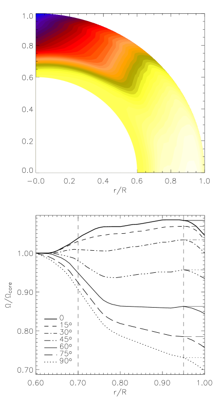
Figure 1: Upper panel: rotation profile adapted from the helioseismic results. The lower panel shows the angular velocity $\Omega$ normalised by the core angular velocity, $\Omega_{\rm core}=430$ nHz, at latitudes $0\degr$ (equator, thick solid line), $15\degr$ (dashed), $30\degr$ (dot-dashed), $45\degr$ (triple-dot-dashed), $60\degr$ (solid), $75\degr$ (long-dashed), and $90\degr$ (pole, dotted line). The dashed vertical lines at $r=0.70R$ and $r=0.95R$ denote the bottom of the convection zone and the depth above which the surface shear layer is located, respectively. The thin horizontal lines above $r=0.95R$ give $\Omega$ in the case where the surface shear is neglected.

3 Results

3.1 Estimates of $C_{\alpha}$ and $C_{\Omega}$ for the Sun

Using the profiles of the transport coefficients from theoretical considerations or local 3D convection calculations, the remaining task is to choose appropriate values for the three dimensionless control parameters $C_{\alpha}$, $C_{\Omega}$, and $C_{U}$, defined via Eq. (9). The local convection calculations of KKOS yield ${\rm max}(|\alpha_{ij}|)/u_{\rm rms}\approx 0.2$. We scale this to physical units by using the mixing length estimate of the turbulent velocity at the bottom of the convection zone, i.e. $u_{\rm rms}^{\rm MLT}\approx 10$ m s^-1, and obtain a magnitude of 2 m s^-1 for $\alpha_{0}$. Furthermore, using the mean angular velocity of the Sun, $\Omega_{0}=2.6\times 10^{-6}$ s^-1, the ratio $C_{\alpha}/C_{\Omega}=\alpha_{0}/(\Omega_{0}R)$ is therefore approximately $10^{-3}$; in the dynamo models describing the Sun, we keep this ratio fixed. Furthermore, the meridional flow at the surface, $u_{0}\approx 10\ldots 20$ m s^-1, is known from observations, from which we obtain another useful ratio for the solar models, i.e. $C_{U}/C_{\Omega}=u_{0}/(\Omega_{0}R)\approx 0.005\ldots 0.01$.

The value of $\eta_{0}$ still remains a free parameter. Simple mixing length estimates for the deep layers of the solar convection zone (e.g. Stix [2002]) give $\eta_{\rm t}=\frac{1}{3}u_{\rm rms}^{\rm MLT}d\approx 5\cdot 10^{8}$ m² s^-1, where $d=\alpha_{\rm MLT}H_{\rm p}$, $\alpha_{\rm MLT}=1.66$, and $H_{\rm p}\approx 5\cdot 10^{7}$ m. Similar or slightly higher values are obtained for all depths in the solar convection zone (see e.g. Brandenburg & Tuominen [1988]). We find that growing solutions are possible when $\eta_{0}\approx 10^{8}$ m² s^-1 (see below).

3.2 Constant $\alpha$ with $\cos{\theta}$ latitude dependence

Although the main emphasis of this paper is to investigate the role of anisotropies found in the local convection models, we perform a set of calculations with a constant $\alpha$-effect in the convection zone with a previously commonly used $\cos{\theta}$ latitude profile in order to demonstrate the current problems of solar mean-field dynamo models. In all of the calculations in this section, we put

$$\alpha_{ij}=\frac{1}{2}\,\alpha_{0}\delta_{ij}\bigg{[}1+\tanh\bigg{(}\frac{r-r_{\rm c}}{d_{1}}\bigg{)}\bigg{]}\cos\theta\;,$$ (16)

where $r_{\rm c}=0.7$ and $d_{1}=0.015$. The $\tanh$-factor takes care of the vanishing $\alpha$-effect in the overshoot region. We study this simple case first and determine the critical dynamo number $C_{\alpha}^{\rm crit}$ as a function of $C_{\Omega}$ for the antisymmetric A0 and symmetric S0 modes. The results for the A0 case are shown in Fig. 2. We note that the critical values for the S0 mode are very close to those of the A0 mode, but consistently slightly larger. The difference, however, is less than one per cent in all cases. For values of $C_{\Omega}$ larger than $10^{4}$ the difference between the $\alpha\Omega$ and $\alpha^{2}\Omega$ models is less than 5 per cent. In what follows we consider the case $C_{\alpha}=15$, $C_{\Omega}=1.5\cdot 10^{4}$ as our standard model, in which case we adopt the $\alpha\Omega$-approximation. Moreover, we note that the critical dynamo number in the case of no surface shear is roughly 20 per cent larger than in the case where it is taken into account.

Figure 2: Critical dynamo numbers $C_{\alpha}^{\rm crit}$ as function of $C_{\Omega}$ for the $\alpha$-profile given by Eq. (16). The solid and dashed lines give the results for the rotation profile including the surface shear, shown in Fig. 1, and using the $\alpha\Omega$ and $\alpha^{2}\Omega$ approximations, respectively. The dot-dashed ($\alpha\Omega$) and triple-dot-dashed ($\alpha^{2}\Omega$) curves give the corresponding results with a rotation profile where the surface shear layer has been removed. The thick solid line describes the Sun, i.e. where $C_{\alpha}/C_{\Omega}=10^{-3}$.

Keeping the ratio $C_{\alpha}/C_{\Omega}$ fixed at $10^{-3}$ we find that the critical dynamo number, $D^{\rm crit}\equiv C^{\rm crit}_{\alpha}C_{\Omega}$, for the excitation of the antisymmetric A0 mode is roughly $D^{\rm crit}\approx 4.89\cdot 10^{4}$ corresponding to $C_{\alpha}^{\rm crit}\approx 6.99$ using the $\alpha\Omega$-approximation ($D^{\rm crit}\approx 4.37\cdot 10^{4}$ corresponding to $C_{\alpha}^{\rm crit}\approx 6.61$ if the $\alpha$-terms are retained in the equation of $B$). In the marginal case the turbulent diffusivity turns out to be $\eta_{0}\approx 2.0\cdot 10^{8}$ m² s^-1. The toroidal magnetic field of the marginal solution exhibits an oscillation period of $t_{\rm cyc}\approx 0.044\tau$, which corresponds to roughly 3.2 years in physical units.

Considering the resulting butterfly diagrams we compare models where the shear above $r=0.95R$ is either turned off (Fig. 3) or retained (Fig. 4). In the former case the butterfly diagram of the azimuthal field near the surface shows that the migration of the activity belts at latitudes $|\Theta|<60\degr$ is poleward with an equatorward branch near the pole, whereas the latter case exhibits a strong equatorward propagating activity belt from latitude $\approx 80\degr$ all the way down to the equator. The migration of the former type has frequently been reported in mean-field models with distributed $\alpha$-effect combined with helioseismological rotation profile (e.g. Bonanno et al. 2002). Concerning the latter case, we note here that if there is a non-vanishing $\alpha$-effect near the surface, the surface shear layer plays a very important role in shaping the butterfly diagram. However, if the $\alpha$-effect is more concentrated in the deep layers of the convection zone the surface shear plays only a minor role (see Sect. 3.5).

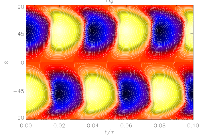
Figure 3: Butterfly diagram of the toroidal magnetic field from $r=0.99R$ from a model with $C_{\alpha}=15$ and $C_{\Omega}=1.5\cdot 10^{4}$ with the rotation profile shown in Fig. 1 with the surface shear at $r>0.95R$ artificially turned off.

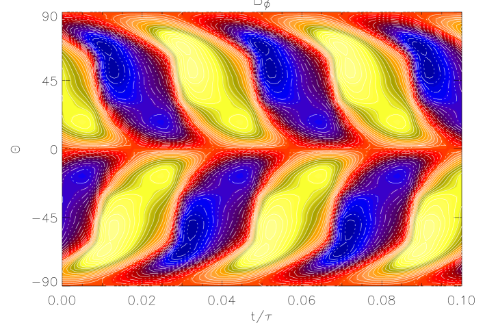
Figure 4: Butterfly diagram of the toroidal magnetic field from $r=0.99R$ from a model with $C_{\alpha}=15$ and $C_{\Omega}=1.5\cdot 10^{4}$ with the full rotation profile shown in Fig. 1. The cycle period is approximately $t_{\rm cyc}\approx 6.5$ years.

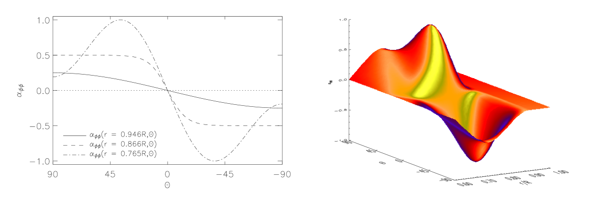
Figure 5: Left panel: profiles of the $\alpha_{\phi\phi}$-component from three depths $r=(0.765,0.866,0.946)R$ corresponding to Coriolis numbers ${\rm Co}=(1,4,10)$, respectively, using the convective velocity at the bottom of the convection zone as normalisation. Right panel: the actual $\alpha_{\phi\phi}(r,\theta)$ profile used in the models.

3.3 $\alpha$-effect from the local convection models

Already the early analytical investigations of the turbulent electromotive force showed that the $\alpha$-effect is highly anisotropic (Steenbeck, Krause & Rädler [1966]). These anisotropies have recently been studied by means of local convection calculations by Ossendrijver et al. ([2002]) and KKOS. In the present study we employ these numerical results of the $\alpha$-effect and turbulent pumping in solar dynamo models. As was discussed earlier, we set the ratio $C_{\alpha}/C_{\Omega}$ to $10^{-3}$ in the case of the solar dynamo. Effectively the small value of the ratio $C_{\alpha}/C_{\Omega}$ means that the dominant (diagonal) component of $\overline{\vec{\alpha}}$ is $\alpha_{\phi\phi}$ which appears in the equation of the poloidal field (see Eqs. 26 and 27). Adopting the $\alpha\Omega$-approximation and setting $\alpha_{\rm rr}=\alpha_{\theta\theta}=0$ does not significantly change our results. These components can, however, be of vital importance for $\alpha^{2}$-dynamos and their oscillation properties such as those investigated by Rüdiger, Elstner & Ossendrijver ([2003]).

In order to make use of the local results of KKOS we use the Coriolis number to determine the depth of the local convection model in the convection zone. In an earlier study we computed the Coriolis number from a mixing-length model of the solar convection zone (Fig. 1 of Käpylä et al. [2005]), and found that it varies between $10^{-3}$ near the surface and $10$ or larger in the deep layers. In KKOS, sets of convection calculations at different latitudes are made with approximate Coriolis numbers of 1, 4, and 10. Identifying these values with depths in the solar convection zone, they correspond to $r=0.946R$, $r=0.866R$, and $r=0.765R$, respectively. In KKOS it was found that for Co = 1 the component corresponding to $\alpha_{\phi\phi}$ is consistent with a $\cos\theta$ latitude profile, whereas for Co = 4 $\alpha_{\phi\phi}$ is basically constant as function of latitude from the poles to the latitude $|\Theta|=30\degr$. In the rapid rotation regime, i.e. Co = 10, $\alpha_{\phi\phi}$ peaks around $|\Theta|=30\degr$ and the magnitude at the poles decreases. We use the following approximations of the latitude dependence of $\alpha_{\phi\phi}$ at the different depths

$$\alpha_{\phi\phi}(r=0.946R,\theta) = \frac{1}{4}\alpha_{0}\cos\theta\;,$$ (17)

$$\alpha_{\phi\phi}(r=0.866R,\theta) = -\frac{1}{2}\alpha_{0}\tanh\bigg{[}4\Big{(}\theta-\frac{\pi}{2}\Big{)}\bigg{]}\;,$$ (18)

$$\alpha_{\phi\phi}(r=0.765R,\theta) = 3\,\alpha_{0}\Big{(}\sin^{2}\theta\cos\theta+\frac{1}{4}\cos\theta\Big{)}\;,$$ (19)

see the left panel of Fig. 5 (see also Figs. 3 to 7 of KKOS). We use cubic spline interpolation in order to obtain a value of $\alpha_{\phi\phi}$ for all grid points, see the right panel of Fig. 5. In Eqs. (17) to (19) an estimate of the convective velocity, $u\approx 10$ m s^-1, at the bottom of the convection zone has been used to scale the profiles at all depths resulting an $\alpha_{\phi\phi}$ profile that peaks near the bottom of the convection zone at around latitude $30\degr$.

Considering models with the $\alpha$-effect depicted in Fig. 5, we find that the critical dynamo number is significantly larger than in the case of constant $\alpha$ in the convection zone, see Fig. 6. Again the critical value for the S0 mode is very sligthly larger than that of the A0 mode. For the solar case of $C_{\alpha}/C_{\Omega}=10^{-3}$ we find $D^{\rm crit}\approx 8.2\cdot 10^{4}$, or $C_{\alpha}^{\rm crit}=9.04$, instead of $D^{\rm crit}\approx 4.89\cdot 10^{4}$ and $C_{\alpha}^{\rm crit}\approx 6.99$ in the case of constant $\alpha_{\phi\phi}$ in the whole convection zone. This is of course due to the fact that the integral of $\alpha_{\phi\phi}$ over the full shell is significantly less than in the case of radially constant $\alpha_{\phi\phi}$. Furthermore, we find that initially purely antisymmetric A0-type configurations are only stable when $C_{\alpha}<12$. In the range $12<C_{\alpha}<17$ the initially purely dipolar A0 solutions evolve towards a symmetric S0 solution after about one diffusion time. Furthermore, when $C_{\alpha}>17$ mixed mode solutions are excited. The butterfly diagrams for the cases $C_{\alpha}<17$ are characterised by strong activity at high latitudes, the maximum being near $50\degr$, see Fig. 7. The migration of the activity belts is equatorward at high latitudes and poleward from the equator up to latitude of about $45\degr$. This demonstrates that the included surface shear layer, leading to equatorward migration in the case of constant in radius $\alpha$-effect, plays a less important role when $\alpha$ concentrates at the bottom of the convection zone. The parameter range within which the dipolar A0 solution is stable in the nonlinear regime is quite narrow. Adding radial and latitudinal components of the pumping vector or a meridional flow pattern is observed to widen this range (see below).

Figure 6: Critical dynamo number $C_{\alpha}^{\rm crit}$ as a function of $C_{\Omega}$ for the antisymmetric A0 mode with the $\alpha$-profile from convection calculations, see Fig. 5 (solid line). The additional curves are with latitudinal and radial pumping according to Eqs. (20) and (21) (dashed line), and with meridional flow according to Eqs. (28) and (29) (dot-dashed line). The thick solid line describes the Sun, i.e. where $C_{\alpha}/C_{\Omega}=10^{-3}$.

3.3.1 Effect of the general pumping effect

The local convection models of KKOS yield all the three components of the pumping vector $\vec{\gamma}$. In the present axisymmetric investigation, the azimuthal pumping $\gamma_{\phi}$, however, would appear only through its radial and latitudinal gradients. These terms would act analogously to the differential rotation but due to the small value of $C_{\alpha}/C_{\Omega}$, these gradients are negligible in comparison to the differential rotation. Therefore we consider here only the radial and latitudinal pumping effects.

According to the local models, the radial pumping is directed downwards throughout the convection zone in the slow and moderate rotation regimes, i.e. ${\rm Co}<4$. The radial pumping velocity is non-zero also in the case of no rotation due to the fact that it is mostly caused by the diamagnetic effect (see e.g. Ossendrijver et al. [2002]). In the slow and moderate rotation regime the dependence on rotation (depth) is indeed rather weak, although $\gamma_{r}$ tends to somewhat increase at the poles and decrease at the equator as function of rotation. The trend is most clear in the rapid rotation regime, i.e. Co = 10, where the radial pumping is very small or even positive at low latitudes and at the equator. In the overshoot region $\gamma_{r}$ vanishes. We adopt a simplified profile which captures the main aspects of the results of KKOS by setting

$$\gamma_{r}(r,\theta) = -\frac{1}{2}\alpha_{0}\bigg{[}\tanh{\Big{(}\frac{r-r_{c}}{d_{1}}\Big{)}}-\tanh{\Big{(}\frac{r-r_{1}}{d_{2}}\Big{)}}\bigg{]}\times$$ (20)

$$\bigg{\{}\exp{\bigg{[}\frac{(r-r_{c})^{2}}{d_{3}^{2}}}\bigg{]}\sin{\theta}+1\bigg{\}}\;,$$

where $r_{c}=0.7$, $r_{1}=0.975$, $d_{1}=0.015$, $d_{2}=0.1$, and $d_{3}=0.25$. The maximum magnitude of the vertical pumping is taken to be the same as that of the $\alpha$-effect, i.e. $\alpha_{0}$, as is suggested by the local results..

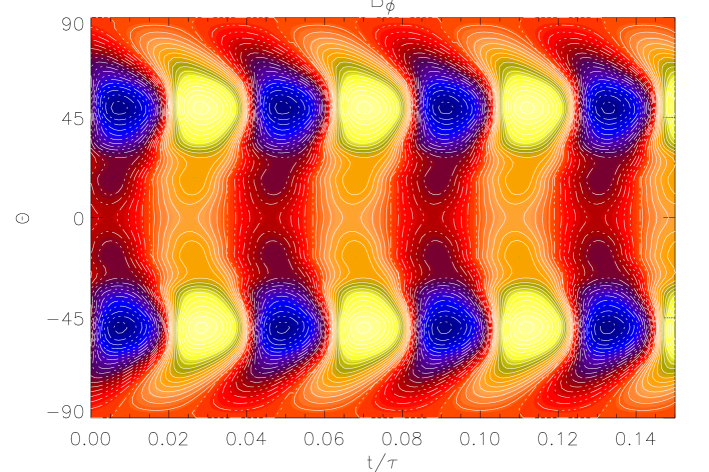
Figure 7: Butterfly diagram of the toroidal magnetic field from $r=0.99R$ from a model with $C_{\alpha}=15$ and $C_{\Omega}=1.5\cdot 10^{4}$. The cycle period is approximately $t_{\rm cyc}\approx 7.0$ years. $\alpha_{\phi\phi}$-profile as shown in Fig. 5.

The latitudinal pumping velocity $\gamma_{\theta}$ is directed equatorwards throughout the convection zone. This effect is rotationally excited (Krause & Rädler [1980]), and thus it shows a strong rotational dependence so that in the bottom of the convection zone it has a peak magnitude of $\approx 2$ m s^-1 whilst it is negligible at the surface. Latitudinally $\gamma_{\theta}$ is strongest near the equator at around $15\degr$ with decreasing values towards the poles. Similarly to the radial component, $\gamma_{\theta}$ vanishes in the overshoot region. We adopt again a simplified profile described by

$$\gamma_{\theta}(r,\theta) = \alpha_{0}\bigg{[}\tanh{\Big{(}\frac{r-r_{c}}{d_{1}}\Big{)}}-\tanh{\Big{(}\frac{r-r_{2}}{d_{4}}\Big{)}}\bigg{]}\times$$ (21)

$$\sin^{4}{\theta}\cos{\theta}\;,$$

where $r_{2}=0.875$ and $d_{4}=0.075$. The magnitude of the pumping effect in the mean-field equations is controlled by the nondimensional parameter $C_{\gamma}$; since the pumping effect is basically a part of the $\alpha$-effect and the maximum magnitudes of both effects were very similar in the study of KKOS we set $C_{\gamma}=C_{\alpha}$.

Adding the pumping velocities defined via Eqs. (20) and (21) into the model already employing the $\alpha$-effect from convection calculations, widens the region in which the dipolar solution is the preferred one (up to $C_{\alpha}\approx 50$). The dashed line in Fig. 6 indicates that the pumping effects make the dynamo easier to excite. This is logical, due to the fact that the radial pumping is generally downward, i.e. towards regions of larger $\alpha$-effect. The latitudinal pumping in the deeper layers has a similar effect, i.e. it transport magnetic fields to lower latitudes. Furthermore, using our standard values $C_{\alpha}=15$ and $C_{\Omega}=1.5\cdot 10^{4}$, the cycle period is also significantly longer in this case, i.e. $t_{\rm cyc}\approx 11$ years instead of approximately seven years in the case without the pumping effects. Another clear effect is that the migration of the activity belts is now equatorward also at low latitudes, see Fig. 8. Both of these results seem to be direct consequences of the added latitudinal pumping; otherwise identical model with $\gamma_{\theta}=0$ yields a butterfly diagram very similar to Fig. 7.

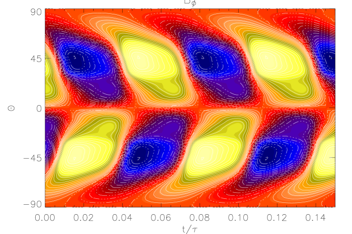
Figure 8: Same as Fig. 7 but with added radial and latitudinal pumping velocities as defined via Eqs. (20) and (21). The cycle period is $t_{\rm cyc}\approx 12$ years.

3.3.2 Effect of field direction dependent pumping effect

The off-diagonal components of the (symmetric) tensor $\overline{\vec{\alpha}}$ contribute to the field direction dependent pumping (Kitchatinov [1991]; Ossendrijver et al. [2002]; KKOS). Therefore, in the general case, we need to introduce $\alpha_{ij}$ components $\alpha_{r\theta}$, $\alpha_{r\phi}$, and $\alpha_{\phi\theta}$ into the model. However, according to the results of KKOS, $\alpha_{\phi\theta}$ is clearly the largest in magnitude of the components entering the equation for $A$. The local calculations show that this component peaks strongly near the equator at or around latitude $15\degr$, and the maximum absolute magnitude is again roughly 2 m s^-1. We introduce a profile

$$\alpha_{\phi\theta}(r,\theta) = -\alpha_{0}\bigg{[}\tanh{\Big{(}\frac{r-r_{c}}{d_{1}}\Big{)}}-\tanh{\Big{(}\frac{r-r_{3}}{d_{2}}\Big{)}}\bigg{]}\times$$ (22)

$$\sin^{12}\theta\cos^{2}\theta\;,$$

where $r_{3}=0.85$ and $d_{2}=0.1$. The main effect of $\alpha_{\phi\theta}$ is that it contributes to the radial pumping of the azimuthal field via $\gamma_{r}^{\phi}=\gamma_{r}-\alpha_{\phi\theta}$, where $\gamma_{r}^{\phi}$ is the pumping velocity for the azimuthal field. The local results of KKOS indicate that the azimuthal field can be pumped upward at latitudes $|\Theta|<45\degr$. Due to the narrow latitude and radius range where $\alpha_{\phi\theta}$ is appreciably large, its effects on the surface are hardly visible (compare Figures 8 and 9).

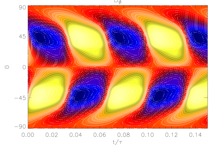
Figure 9: Same as Fig. 8 but with added field direction dependent pumping according to Eq. (22). The cycle period is about 12 years.

3.4 Effect of meridional flow

Solar surface indicators and local helioseismology (Zhao & Kosovichev [2004]; Komm et al. [2004]) have revealed that there is a mean poleward flow of 10–20 m s^-1 near the solar surface. Although no observational evidence exists as of yet, it is generally accepted that there is a return flow at some greater depth. However, it is also not known whether there is only one cell in radius or more. The simplest case is to assume that there is only one cell. We adopt a modified version of the flow used by Dudley & James ([1989]), defined via a potential for the poloidal flow

$$\psi=x^{2}\sin(\pi x)P_{2}^{0}(\cos\theta)\;,$$ (23)

where $x=(r-r_{c})/(R-r_{c})$, and $P_{2}^{0}(\cos\theta)=\frac{1}{2}(3\cos^{2}\theta-1)$. Here $x$ describes the effect of decreasing density towards the top of the convection zone. The radial and latitudinal velocity components are obtained via

$$u_{r} = -\frac{1}{r^{2}\sin\theta}\frac{\partial}{\partial\theta}\Big{(}\sin\theta\frac{\partial\psi}{\partial\theta}\Big{)}\;,$$ (24)

$$u_{\theta} = \frac{1}{r}\frac{\partial}{\partial r}\frac{\partial\psi}{\partial\theta}\;,$$ (25)

which are written out explicitly in Eqs. (28) and (29) in Appendix A.

Fixing the maximum value of the flow at the surface to 10 m s^-1 yields $C_{U}=75$ or $C_{U}/C_{\Omega}=0.005$ for the standard model where $C_{\alpha}=15$. Introducing this flow into the model discussed in Sect. 3.3.2 which already includes both pumping effects, we obtain the butterfly diagram shown in Fig. 10. The most visible effect of the meridional flow is the appearance of the polar branch at latitudes $\Theta>60\degr$. Furthermore, the equatorward propagating activity belts appear now at slightly lower latitudes, although the difference to the observed solar activity is still quite large. The critical dynamo numbers in the case with meridional flow are in general somewhat higher than in the case with only radial and latitudinal pumping taken into account. Furthermore, when $C_{\Omega}$ is smaller than approximately $1.5\cdot 10^{4}$, the symmetric S0 mode is somewhat easier to excite than the A0 mode (not shown).

In the nonlinear regime the solution is dipolar (A0) for $C_{\alpha}<15$, quadrupolar in the range $C_{\alpha}\approx 15\ldots 30$, and mixed parity solutions are obtained when $C_{\alpha}>30$ keeping the ratio $C_{U}/C_{\Omega}=0.005$ fixed. If $C_{U}/C_{\Omega}$ is incereased the activity belts are shifted closer to the equator, but the S0 and mixed modes become somewhat easier to excite. Increasing the dynamo numbers is associated with an increasing cycle period, but with the present profiles for the $\alpha$-effect and turbulent pumping the solutions in the solar range, i.e. $t_{\rm cyc}\approx 22$ years, all consist of mixed modes.

We note here that in the present models the magnetic Reynolds number is equal to $C_{U}$, i.e. ${\rm Rm}=C_{U}\approx\mathcal{O}(100)$. This means that we are not in the advection dominated regime realised in many flux transport dynamo models (e.g. Dikpati & Charbonneau [1999]; Bonanno et al. [2002]) where values in excess of $10^{3}$ are common. The value of Rm, however, indicates that the present models are also not fully diffusion dominated, but rather represent a distributed dynamo.

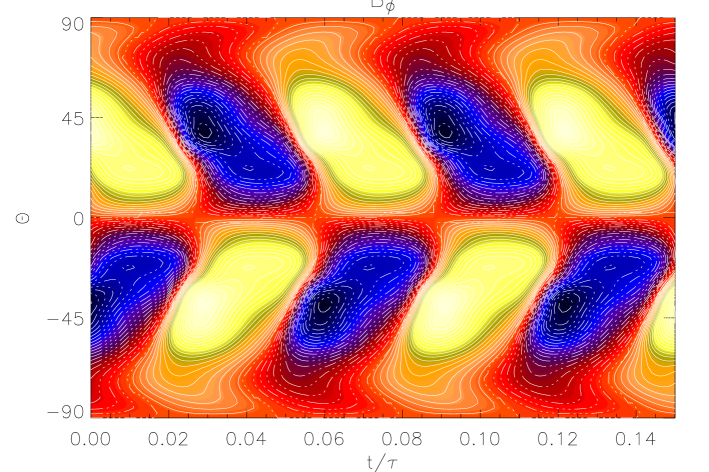
Figure 10: Same as Fig. 9 but with added meridional flow with max($u_{\theta}$) = 10 m s^-1 at the surface, with which choice $C_{U}=75$. The cycle period is about 11.5 years.

3.5 The effect of the surface shear layer

In order to study the influence of the surface shear layer on the solution we take the same setup as in the previous section and turn off the shear above $r=0.95R$. The resulting butterfly diagram is shown in Fig. 11. Comparing this with Fig. 10 shows some differences, most visibly the less extended active regions, and a narrow region of poleward migration near the equator. In contrast to the case of uniformly distributed $\alpha$-effect (see Sect. 3.2) for which case the surface shear plays a significant role, the importance of the surface shear is very small if the $\alpha$-effect more concentrated near the bottom of the convection zone.

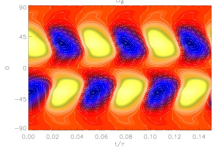
Figure 11: Same as Fig. 10 where the surface shear above $r=0.95R$ has been artificially turned off. The cycle period is about 9.5 years.

3.6 Phase relation of $B_{r}B_{\phi}$

We note briefly that in our models the correlation of the radial and azimuthal magnetic field components, i.e. $B_{r}B_{\phi}$, is mostly negative (see Fig. 12 for a typical result) in the latitude range where the activity belts are located in accordance with solar observations (e.g. Stix [1976]). This relation has commonly been used as a constraint for solar dynamo models (e.g. Stix [1976]; Schlichenmaier & Stix [1995]; Brandenburg [2005]) although this has recently been criticized by Schüssler ([2005]) who explains this relation as the consequence of the systematic tilt of the bipolar regions due to the action of Coriolis force on rising flux ropes in the convection zone.

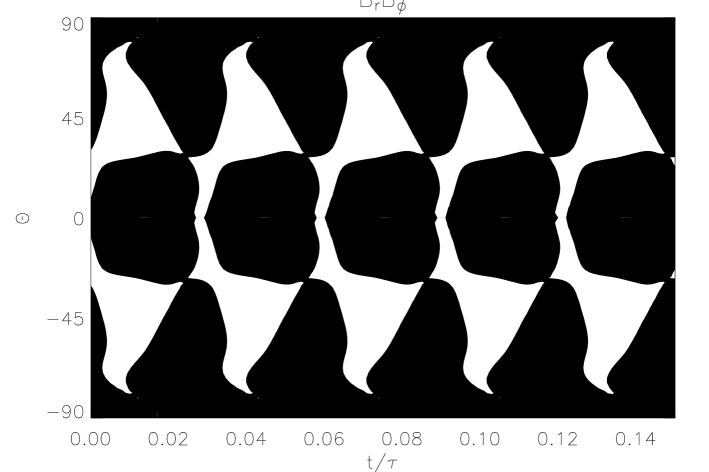
Figure 12: The correlation $B_{r}B_{\phi}$ from the model shown in Fig. 10. Black denotes negative and white positive values.

4 Conclusions

We have studied kinematic mean-field solar dynamo models using helioseismologically determined rotation profile and $\alpha$-effect and turbulent pumping from the local convection calculations of Käpylä et al. ([2006]). We show that if a simple $\alpha$-effect profile proportional to $\cos\theta$ in latitude and constant in radius is applied, the results are very sensitive to the presence of a surface shear layer at $r>0.95R$. Omitting this feature, the migration of the activity belts is equatorward near the poles, weak at midlatitudes, and poleward at low latitudes. The inclusion of the shear layer results in equatorward propagation at virtually all latitudes.

The $\alpha$-coefficients from local convection calculations tend to be much more concentrated near the bottom of the convection zone and also closer to the equator with peak values occuring at around latitude $30\degr$. In this case, however, the critical dynamo numbers are significantly larger due to the more concentrated nature of the $\alpha$-effect. The solution is dipolar when $C_{\alpha}<12$ and quadrupolar (S0) if $C_{\alpha}$ is larger even if a purely dipolar initial condition is used. Adding a latitudinal pumping velocity of the order of 2 m s^-1 at the bottom of the convection zone remedies this problem and helps to shift the activity belts closer to the equator, whereas the vertical pumping seems to have a much smaller overall signifigance for the stability and overall structure of the solution. The latitudinal pumping also helps to restore the equatorward migration of activity belts, lost by the implementation of the $\alpha$-effect from convection calculations. Adding the pumping effects also makes the cycle period significantly longer. Additional upward pumping of the azimuthal field component through the component $\alpha_{\phi\theta}$ at near equator regions has very little effect on the solution. In all the models investigated, the correlation $B_{r}B_{\phi}$ is mostly negative, which is in agreement with the observations, but none of the models produces poleward migration at high latitudes (polar branch).

If a single cell meridional flow patterns where the flow is of the order of 10 m s^-1 and poleward near the surface and significantly smaller and equatorward at larger depths helps to shift the activity belts further closer to the equator, although they still appear too high ($|\Theta|\approx 5\degr\ldots 60\degr$) in comparison to the Sun. A region of poleward migration also appears at high latitudes. If the upper shear layer is removed from this model, the butterfly diagram changes only little in contrast to the models where there was an appreciably large $\alpha$-effect also near the surface.

The distributed dynamo model investigated in this paper correctly reproduces many of the general features of the solar cyclic activity, including realistic migration patterns and correct phase relation, but some problems persist. These include the excitation of the dipolar (A0) solutions only within a narrow range of parameters with the anisotropic $\alpha$-effect combined with meridional circulation, activity at too high latitudes for all models investigated, and the somewhat too short dynamo cycles. With further tuning of the various parameters going into the model (magnitudes of $\alpha$- and $\gamma$-effects, strength and profile of the meridional circulation) it would most likely be possible to obtain a solution reproducing the missing features, as well. Instead of going further into the domain of tuning in the present study, we note that further work in the context of local convection modelling is needed in order to obtain the totally missing information on the anisotropies of turbulent diffusivity (work in progress). It is also necessary to consider the nonlinear saturation process of the $\alpha$-effect in more detail, for instance in the form of a dynamical $\alpha$-effect with helicity fluxes (e.g. Brandenburg & Subramanian [2005]). Further improvements of the present mean-field model include the relaxation of the kinematic approach to include full dynamics, for which purpose information from local convection calculations also exist (e.g. Käpylä, Korpi & Tuominen [2004]). With the inclusion of hydro- and thermodynamics the nonlinear feedbacks of the kind investigated by e.g. Rempel ([2006]) could be included in a self-consistent way.

Despite of the shortcomings discussed above, we feel that the simple model presented in this paper demonstrates two important aspects concerning solar dynamo theory. Firstly, as recently discussed at length by Brandenburg ([2005]) the surface shear layer may be important in shaping the solar dynamo; according to our results this is indeed to be expected if the $\alpha$-effect has an appreciable magnitude near the surface. Secondly, we are able to demonstrate that a distributed $\alpha\Omega$-dynamo model applying a realistic rotation profile and meridional flow can reproduce the correct phase relation and migration of the activity belts. Although meridional circulation is an essential ingredient also in our model, the magnitude of this effect is of the same order as the turbulent inductive effects and the turbulent diffusivity is an order of magnitude larger than in the advection dominated flux-transport dynamos.

Appendix A Equations

The equation for $A$ reads

$$\frac{\partial A}{\partial\tau} = (C_{\alpha}\alpha_{\phi\theta}-C_{U}U_{r})\bigg{(}\frac{A}{r}+\frac{\partial A}{\partial r}\bigg{)}$$ (26)

$$+ (C_{\alpha}\alpha_{\phi r}-C_{U}U_{\theta})\bigg{(}\frac{\cot\theta}{r}A+\frac{1}{r}\frac{\partial A}{\partial\theta}\bigg{)}$$

$$+ C_{\alpha}\alpha_{\phi\phi}B$$

$$+ \eta_{t}\bigg{(}\frac{\partial^{2}A}{\partial r^{2}}+\frac{2}{r}\frac{\partial A}{\partial r}+\frac{1}{r^{2}}\frac{\partial^{2}A}{\partial\theta^{2}}+\frac{\cot\theta}{r^{2}}\frac{\partial A}{\partial\theta}$$

$$- \frac{A}{r^{2}\sin^{2}\theta}\bigg{)}\;,$$

where $U_{i}=U^{mer}_{i}+\frac{C_{\gamma}}{C_{U}}\gamma_{i}$.

$$\frac{\partial B}{\partial\tau} = C_{\Omega}r\sin\theta\bigg{[}\frac{\partial\Omega}{\partial r}\Big{(}\frac{\cot\theta}{r}A+\frac{1}{r}\frac{\partial A}{\partial\theta}\Big{)}\bigg{]}$$ (27)

$$- C_{\Omega}\sin\theta\bigg{[}\frac{\partial\Omega}{\partial\theta}\Big{(}\frac{A}{r}+\frac{\partial A}{\partial r}\Big{)}\bigg{]}$$

$$- C_{U}\frac{U_{r}B}{r}+C_{U}\frac{1}{r}\frac{\partial U_{\phi}}{\partial r}\Big{(}\cot\theta A+\frac{\partial A}{\partial\theta}\Big{)}$$

$$+ C_{U}\frac{U_{\phi}}{r}\Big{(}\cot\theta\frac{\partial A}{\partial r}-\frac{1}{r}\frac{\partial A}{\partial\theta}\Big{)}-C_{U}\frac{1}{r}\frac{\partial U_{\phi}}{\partial\theta}\Big{(}\frac{A}{r}+\frac{\partial A}{\partial r}\Big{)}$$

$$- C_{U}\bigg{(}\frac{\partial U_{r}}{\partial r}B+U_{r}\frac{\partial B}{\partial r}\bigg{)}-C_{U}\frac{1}{r}\bigg{(}\frac{\partial U_{\theta}}{\partial\theta}B+U_{\theta}\frac{\partial B}{\partial\theta}\bigg{)}$$

$$+ C_{\alpha}\bigg{(}\frac{\alpha_{\theta r}}{r}+\frac{\partial\alpha_{\theta r}}{\partial r}-\frac{1}{r}\frac{\partial\alpha_{rr}}{\partial\theta}\bigg{)}\bigg{(}\frac{\cot\theta A}{r}+\frac{1}{r}\frac{\partial A}{\partial\theta}\bigg{)}$$

$$- C_{\alpha}\bigg{(}\frac{\alpha_{\theta\theta}}{r}+\frac{\partial\alpha_{\theta\theta}}{\partial r}-\frac{1}{r}\frac{\partial\alpha_{r\theta}}{\partial\theta}\bigg{)}\bigg{(}\frac{A}{r}+\frac{\partial A}{\partial r}\bigg{)}$$

$$+ C_{\alpha}\bigg{(}\frac{\alpha_{\theta\phi}}{r}+\frac{\partial\alpha_{\theta\phi}}{\partial r}-\frac{1}{r}\frac{\partial\alpha_{r\phi}}{\partial\theta}\bigg{)}B$$

$$- C_{\alpha}\frac{\alpha_{rr}}{r}\bigg{(}\frac{A}{r\sin^{2}\theta}-\cot\theta\frac{\partial A}{\partial\theta}-\frac{\partial^{2}A}{\partial\theta^{2}}\bigg{)}$$

$$- C_{\alpha}\alpha_{\theta\theta}\bigg{(}\frac{A}{r^{2}}-\frac{1}{r}\frac{\partial A}{\partial r}-\frac{\partial^{2}A}{\partial r^{2}}\bigg{)}$$

$$- C_{\alpha}\bigg{[}\alpha_{\theta r}\frac{\cot\theta}{r}\bigg{(}\frac{A}{r}+\frac{\partial A}{\partial r}\bigg{)}-\alpha_{\theta\phi}\frac{\partial B}{\partial r}+\frac{\alpha_{r\phi}}{r}\frac{\partial B}{\partial\theta}\bigg{]}$$

$$+ \eta_{t}\bigg{(}\frac{\partial^{2}B}{\partial r^{2}}+\frac{2}{r}\frac{\partial B}{\partial r}+\frac{1}{r^{2}}\frac{\partial^{2}B}{\partial\theta^{2}}+\frac{\cot\theta}{r^{2}}\frac{\partial B}{\partial\theta}$$

$$- \frac{B}{r^{2}\sin^{2}\theta}\bigg{)}\;.$$

The meridional flow components are given by

$$u_{r} = 6\frac{x^{2}}{r^{2}}\sin(\pi x)\bigg{(}\frac{3}{2}\cos^{2}\theta-\frac{1}{2}\bigg{)}\;,$$ (28)

$$u_{\theta} = -3\frac{x}{r(R-r_{\rm c})}[2\sin(\pi x)+\pi x\cos(\pi x)]\sin\theta\cos\theta\;.$$ (29)