A re-analysis of the three-year Wilkinson Microwave Anisotropy Probe temperature power spectrum and likelihood

Abstract

We analyze the three-year WMAP temperature anisotropy data seeking to confirm the power spectrum and likelihoods published by the WMAP team. We apply five independent implementations of four algorithms to the power spectrum estimation and two implementations to the parameter estimation. Our single most important result is that we broadly confirm the WMAP power spectrum and analysis. Still, we do find two small but potentially important discrepancies: On large angular scales there is a small power excess in the WMAP spectrum (5–10% at $\ell\lesssim 30$) primarily due to likelihood approximation issues between $13\leq\ell\lesssim 30$. On small angular scales there is a systematic difference between the V- and W-band spectra (few percent at $\ell\gtrsim 300$). Recently, the latter discrepancy was explained by Huffenberger et al. (2006) in terms of over-subtraction of unresolved point sources. As far as the low-$\ell$ bias is concerned, most parameters are affected by a few tenths of a sigma. The most important effect is seen in $n_{\textrm{s}}$. For the combination of WMAP, Acbar and BOOMERanG, the significance of $n_{\textrm{s}}\neq 1$ drops from $\sim 2.7\sigma$ to $\sim 2.3\sigma$ when correcting for this bias. We propose a few simple improvements to the low-$\ell$ WMAP likelihood code, and introduce two important extensions to the Gibbs sampling method that allows for proper sampling of the low signal-to-noise regime. Finally, we make the products from the Gibbs sampling analysis publically available, thereby providing a fast and simple route to the exact likelihood without the need of expensive matrix inversions.

1. Introduction

Very recently, the Wilkinson Microwave Anisotropy Probe (WMAP) team released the results from three years of observations of the cosmic microwave background (Hinshaw et al., 2006; Page et al., 2006; Spergel et al., 2006). In addition to improving upon the successful first-year release (Bennett et al., 2003a), this new data set includes the first full-sky polarization maps at millimeter wavelengths (Page et al., 2006), and is destined to be of great importance for the CMB community for many years to come.

Given the dominant position of the WMAP experiment in our current understanding of cosmology, it is imperative that all of the results are verified by several external groups using independent techniques. In this paper we begin these efforts by re-computing the angular power spectrum and likelihoods, arguably the two most important products of any CMB experiment. Similar work was carried out after the first-year WMAP release in 2003 by several groups (e.g., Slosar, Seljak and Makarov, 2004 – the importance of foreground marginalization at large scales; O’Dwyer et al. 2004 – the importance of exact likelihood/posterior evaluation at large scales; Fosalba and Szapudi 2004 – pixel space versus harmonic space computations). These analyses significantly contributed to the improvements that were implemented for the three-year WMAP data release (Hinshaw et al., 2006).

Our philosophy in the present paper is that of multiple redundancy and cross-checking: For both the angular power spectrum and the likelihoods (or posteriors) we apply several different algorithms and in some cases different implementations of the same algorithm. Additionally, the data were downloaded, prepared and analyzed by five independent groups, further reducing the risk of both programming errors, simple misunderstandings and algorithmic peculiarities. This increases our confidence in the final results.

One question that will be given particular attention is the issue of statistical and numerical procedure. Examples are, how should a high signal-to-noise but low-$\ell$ likelihood be regularized at its small scale cut-off in order to avoid numerical artifacts? And in what $\ell$-range does a pseudo-spectrum estimator provide an adequate approximation to the full posterior, and where should an exact approach (such as Gibbs sampling) be preferred?

A separate question is the problem of foreground modeling and subtraction. This will be considered in greater detail in a future publication, and for now we mainly adopt the approaches used by the WMAP team, with one or two notable exceptions: A power spectrum that does not rely on external information (Saha et al., 2006) is established and used as a cross-check on the results that are obtained from template-corrected maps, and we compare spectra computed for different frequencies in order to search for frequency-dependent signatures.

Another major part of the three-year WMAP release are measurements of the CMB polarization (Page et al., 2006). This is a very complex data set, and requires a high degree of algorithmic sophistication for proper interpretation. The necessary extensions to the methods described in the present paper are currently being developed, and the results from the corresponding analyses will be reported upon as soon as they are completed. In the present paper, we focus on temperature information only.

The rest of the paper is organized as follows. In Section 2 we briefly list the methods we use, and in Section 3 we describe the data. Then, we focus on the low-$\ell$ part of the power spectrum in Section 4 and the high-$\ell$ part in Section 5. Cosmological parameters are considered in Section 6, before drawing conclusions in Section 7. Algorithmic details are deferred to two Appendices.

2. Methods

In this paper we are primarily interested in scientific results, and less in algorithms as such. In this section we only list each method that we use, and provide more details in the Appendices where necessary, or with references to earlier papers.

Low-$\ell$ likelihood evaluation

A central component for several of our methods is evaluation of the full likelihood $\mathcal{L}$ in pixel-space which is defined by

$$-2\log\mathcal{L}=\mathbf{d}^{t}\mathbf{C}^{-1}\mathbf{d}+\log|\mathbf{C}|.$$ (1)

up to a normalization constant. Here $\mathbf{d}$ are the observed data in a pixelized form and $\mathbf{C}$ is the corresponding covariance matrix. Evaluation of this quantity involves computing a matrix inverse and determinant, and therefore scales as $\mathcal{O}(N_{\textrm{pix}}^{3})$, $N_{\textrm{pix}}$ being the number of pixels in the data set. Consequently, likelihood evaluations are only feasible at low resolutions, and the data must be degraded prior to analysis. Full details on this operation are given in Appendix A. Regularization of the covariance matrix with respect to the Nyquist frequency is an issue worth some consideration and we do this by wide-beam smoothing and noise addition. This is to be contrasted to the approach used by the WMAP likelihood code that goes beyond the Nyquist frequency to achieve a similar effect (Hinshaw et al., 2006). For further comments on this issue, see Section 4 and Appendix A.

Maximum–likelihood estimation

The maximum-likelihood (ML) power spectrum is simply the one that maximizes the likelihood as defined by Equation 1. This may be found by any non-linear search algorithm, and for the present paper we have used both a quasi-Newton and a Sequential Quadratic Programming algorithm for this task. We obtain identical results with the two methods. Previous analyses using similar techniques include Gorski et al. (1996), Bond et al. (1998), Efstathiou (2004), Slosar et al. (2004) and Hinshaw et al. (2006).

Posterior mapping by MCMC

Alternatively, we may choose a Bayesian approach and map out the entire posterior distribution $P(C_{\ell}|\mathbf{d})\propto\mathcal{L}(C_{\ell})P(C_{\ell})$. Here $P(C_{\ell})$ is a prior on the power spectrum, which is chosen to be uniform in the following. Such mapping may be done very conveniently with Markov Chain Monte Carlo (MCMC) techniques. Some example CMB applications of MCMC techniques are described by Knox et al. (2001), Lewis & Bridle (2002) and Eriksen et al. (2006).

Posterior mapping by Gibbs sampling

As mentioned above, a direct likelihood evaluation scales as $\mathcal{O}(N_{\textrm{pix}}^{3})$, and the two above algorithms are therefore limited to low resolution maps. Fortunately, it is possible to circumvent this problem through a technique called Gibbs sampling that allows for sampling from $P(C_{\ell},\mathbf{s}|\mathbf{d})$, $\mathbf{s}$ being the CMB signal, through the conditional distributions $P(C_{\ell}|\mathbf{s},\mathbf{d})$ and $P(\mathbf{s}|C_{\ell},\mathbf{d})$. The conditional nature of the algorithm avoids inversion of large $\mathbf{S}+\mathbf{N}$ matrices that are dense in all bases. It thereby achieves the same goal as the above MCMC technique with drastically reduced demand on computational resources (Jewell et al., 2004; Wandelt et al., 2004; Eriksen et al., 2004).

MASTER

Approaching the power spectrum estimation problem from a fundamentally different angle, the pseudo-$C_{\ell}$ methods (e.g., MASTER; Hivon et al. 2002) simply 1) compute the spherical harmonics expansion with partial sky data; 2) form a raw quadratic estimate of the power spectrum; 3) correct for noise; and 4) finally decouple the mode correlations by means of an analytically computable coupling kernel. Such methods have proved to be very useful tools for CMB analysis, primarily due to their low computational cost, which again allows for massive Monte Carlo simulations.

MASTER with cross-spectra

For multi-channel experiments, a straightforward and very useful extension to the original MASTER algorithm is simply to include only cross-correlations between channels in the power spectrum estimate (Hinshaw et al., 2003). While an auto-correlation implementation is quite sensitive to assumptions in the noise model, such assumptions only affect the error bars in a cross-spectrum and not the mean.

MASTER with internal foreground cleaning

For multi-frequency experiments with multiple channels per frequency it is possible to form a set of foreground-cleaned maps using different channels within each frequency. The noise contributions are thus still uncorrelated among several pairs of cleaned maps, and the cross-correlation MASTER implementation may be applied as described above even to these maps. Such a method was implemented by (Saha et al., 2006) using the foreground cleaning method of Tegmark et al. (2003). We use this method in the present paper for monitoring residual foregrounds in the spectra computed with template-cleaned maps, and will refer to the method as “MASTER with internal cleaning” (MASTERint for short; MASTERext refers to foreground correction by external templates).

3. Data

The WMAP temperature data (Hinshaw et al., 2006) are provided in the form of ten sky maps observed at five frequencies between 23 and 94 GHz. These maps are pixelized at HEALPix resolution parameter $N_{\textrm{side}}=512$ resulting in about 3 million pixels per map. In this paper we mainly consider the V-band (61 GHz) and W-band (94 GHz) channels since these are the ones with the lowest foreground contamination levels. However, the full data set is used by MASTERint.

We take into account the (assumed circularly symmetric) beam profile of each channel independently, and we adopt the Kp2 sky cut as our base mask. This excludes 15.3% of the sky including all resolved point sources. However, for the low-resolution analyses we consider downgraded and/or expanded versions of this mask. The details of the degradation procedure will be discussed later.

The noise is modeled as uncorrelated, non-uniform and Gaussian with an RMS given by $\sigma_{0,i}/\sqrt{N_{\textrm{obs}}(p)}$. Here $\sigma_{0,i}$ is the noise per observation for channel $i$, and $N_{\textrm{obs}}(p)$ is the number of observations in pixel $p$. However, this approximation is not adequate for all channels, and in particular the W-band must be treated with special care because of significant noise correlations.

We consider two different foreground correction procedures. First, we simply use the template-corrected maps as provided on the LAMBDA website, from which a free-free template (Finkbeiner, 2003), a dust template (Finkbeiner et al., 1999) and the K-Ka WMAP sky map have been fitted and subtracted. Second, to cross-check these results we include a MASTER implementation that does not rely on any external information (Saha et al., 2006).

Finally, the power spectrum contributions from unresolved point sources are subtracted band-by-band as a post-processing step according to the model described by Hinshaw et al. (2006).

4. Large-scale analysis

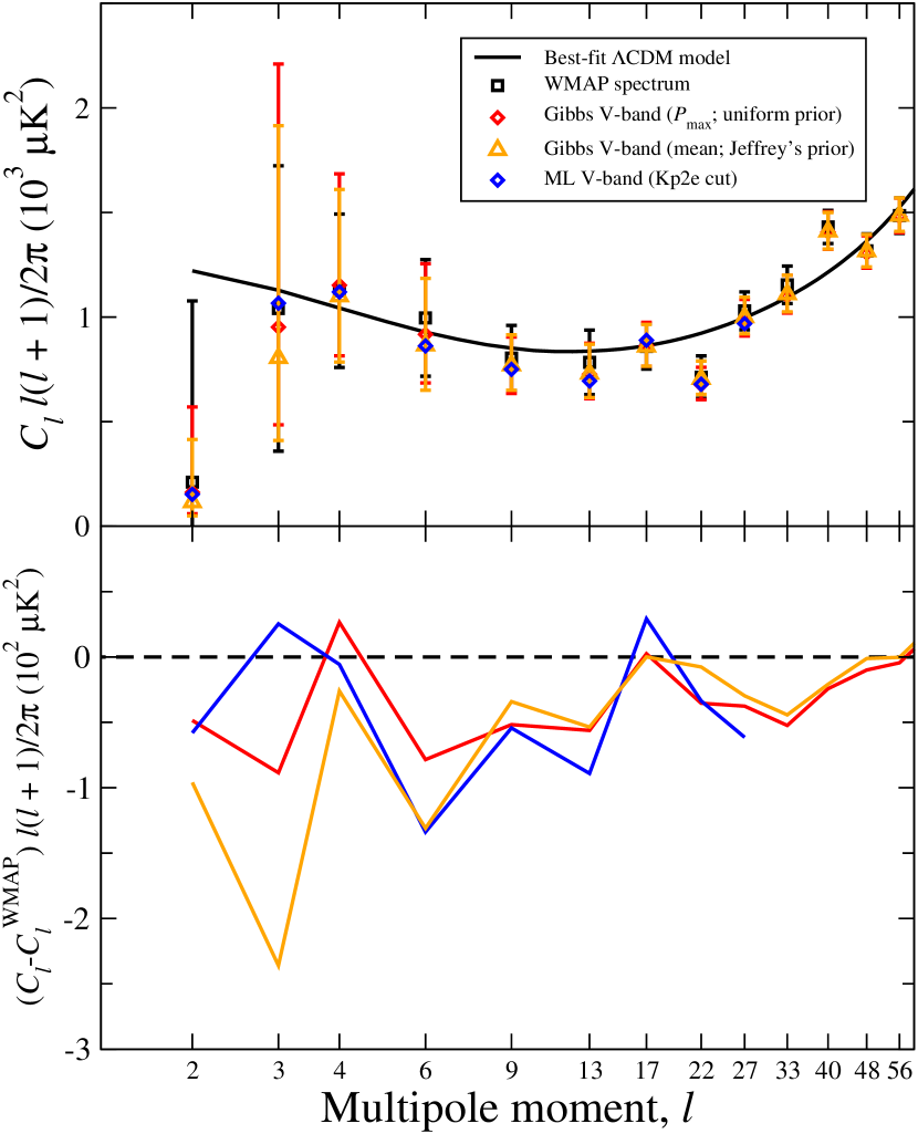
Figure 1.— Top panel: Comparison of low-$\ell$ power spectra computed from the three-year WMAP data using different techniques and data combinations. Bottom panel: Differences between the spectra computed in this paper and the (appropriately binned) WMAP spectrum. See text for full details.

In this section we present the results from our large-scale analyses, broadly defined by $\ell\lesssim 50$. The high-resolution results are shown in Section 5.

4.1. Pre-processing and data selection

Since pixel-space likelihood evaluations scale as $\mathcal{O}(N^{3}_{\textrm{pix}})$, we require low-resolution data for both the maximum-likelihood and MCMC analyses. For these methods, we therefore consider downgraded maps at $N_{\textrm{side}}=16$, each having 3072 pixels on the full sky. For Gibbs sampling, angular resolution does not carry a similar resolution-dependent computational cost, and the analysis is made with full-resolution data. MASTER results are ignored until the next section, since they are sub-optimal and difficult to compare with other estimates at large angular scales. However, we note that we have reproduced the MASTER spectra presented by the WMAP team exactly with MASTERext, and very closely with MASTERint.

The full-resolution sky maps were downgraded as follows. (See Appendix A for a thorough discussion of this procedure.) First, the full resolution maps were de-convolved by the instrumental beam and $N_{\textrm{side}}=512$ pixel window, and then re-convolved by a Gaussian $9^{\circ}$ FWHM beam and $N_{\textrm{side}}=16$ pixel window. Finally, uniform Gaussian noise with a standard deviation of $1\,\mu\textrm{K}$ was added to each pixel. This ensures that the map is properly bandwidth limited at $\ell_{\textrm{max}}=3\cdot N_{\textrm{side}}=48$ and noise dominated beyond $\ell=40$.

The full-resolution Kp2 mask was downgraded in two different ways. In the first case, we set excluded pixels to zero and included pixels to unity. Then we downgrade the mask using the hierarchical structure of HEALPix, and set each low-resolution pixel to the average of all sub-pixels. If this average is larger than 0.5, the low-resolution pixel is accepted. This is the method used in the WMAP likelihood code, and will be denoted by “Kp2” in the following. (In order to compare directly to the WMAP results, we first downgrade to $N_{\textrm{side}}=8$, and then upgrade to $N_{\textrm{side}}=16$, ensuring identical sky masks.) In the second case, we smooth the original mask by a Gaussian beam of $9^{\circ}$ FWHM, project the smoothed field onto the low-resolution grid, and reject all pixels with a value smaller than 0.991, roughly expanding the original mask by one FWHM in all directions. This mask will be denoted “Kp2e” in the following – “e” for extended – and excludes about 7% more pixels than the Kp2 mask.

We consider three maps in these analyses, namely the de-biased Internal Linear Combination (ILC) map and the template-corrected V- and W-band maps individually. Instrumental noise is negligible at these scales, and co-addition is neither required nor desirable. The non-zero frequency range is instead used for foreground monitoring.

In order to further minimize the impact of foregrounds, we adopt the approach of the WMAP team, and construct a foreground template as the difference between the raw V-band and the ILC map. This template is then downgraded in a similar manner as the data maps, but without noise addition. A corresponding term is added to the covariance matrix with a large pre-factor in order to remove any sensitivity to fluctuations with the same spatial pattern as the template (e.g., Bond et al. 1998 and Appendix A).

4.2. Specification of algorithms

Three different algorithms are used for the low-$\ell$ analysis, namely Gibbs sampling, Maximum Likelihood (ML) estimation with low-resolution data, and MCMC with low-resolution data. In the first case, two different implementations are used (Commander and MAGIC; Eriksen et al. 2004) using different priors. In both cases, the power spectra were refined using the Blackwell-Rao estimator (Chu et al., 2005). For Commander, we use uniform priors, and report the modes of the posterior distributions as the power spectrum estimates. This may be directly compared to the WMAP spectrum which is claimed to be a maximum-likelihood estimate at low $\ell$’s. For MAGIC, we use the Jeffrey’s ignorance prior, and report the means as our power spectrum estimates. In either case, we adopt asymmetric 68% confidence regions as our uncertainties.

The ML estimates are established by means of two different non-linear search algorithms from a commercial library, one quasi-Newton method and one sequential quadratic programming method. The free parameters are the binned $C_{\ell}$’s (adopting the binning scheme used by the WMAP team) up to $\ell=30$, for a total of 9 free variables. From $\ell=31$ the spectrum is fixed at the WMAP spectrum values. The covariance matrix is defined as detailed in Appendix A, and consists of a sum of a CMB signal term, a noise term and a foreground (monopole, dipole and ILC–V difference map) term.

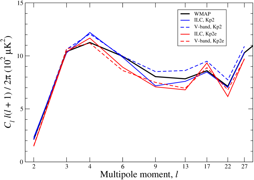
Figure 2.— Power spectrum dependence on sky cut and data set. Colored lines show the maximum likelihood spectra (computed with a pixel-based likelihood) for different sky cuts (blue – directly downgraded Kp2; red – expanded Kp2) and data sets (dashed – ILC; solid – V-band). Note that the expanded Kp2 mask spectra lies systematically below the directly downgraded Kp2 mask spectra.

The MCMC analysis is identical to the ML analysis in terms of the likelihood evaluation method, binning scheme, multipole range etc., but uses a Metropolis-Hastings algorithm to probe the full posterior distribution. We adopt a uniform prior even in this case. Eight independent chains are run for 100 000 steps each, ensuring excellent convergence properties. One single step costs approximately 1 CPU second for a 2000 pixel data set.

4.3. Results

In Figure 1 we show a comparison of four different low-$\ell$ power spectrum estimates: The WMAP spectrum (black), the Commander posterior mode uniform prior V-band spectrum (red), the MAGIC posterior mean Jeffrey’s prior V-band spectrum (orange), and the ML V-band spectrum computed with the Kp2e mask (blue). In the bottom panel, we show the differences taken between these spectra and the WMAP spectrum. Error bars are only shown in the top panel: All analyses study the same data set, and cosmic variance uncertainties can therefore not be used to compare the relative agreement between the various solutions.

First we note that the individual variations between all four spectra are about 50-100$\,\mu\textrm{K}^{2}$, corresponding to about 5-10% of the absolute spectrum amplitude. This is much less than the cosmic variance, and the analysis uncertainty per mode is thus not a dominant effect. However, it is troublesome that this difference appears to be systematic: All three colored spectra lie below the WMAP spectrum up to $\ell\approx 30-40$. Since the cumulative effect over an entire multipole decade of even a small bias may potentially affect cosmological parameters, it is important to determine the origin of this discrepancy.

Foreground uncertainties are always a concern at large angular scales for CMB experiments and a most natural first candidate to consider. First, we note that the four spectra shown in Figure 1 are computed from slightly different data sets: The WMAP spectrum is based on the ILC map with a directly downgraded (i.e., not expanded) Kp2 mask for $\ell\leq 12$ and on the template-corrected V- and W-bands with the high-resolution Kp2 cut at $\ell>12$; the Gibbs spectra are based on the template-corrected V-bands and the full-resolution Kp2 cut at all scales; the ML estimate is computed from the degraded template-corrected V-band, cut with the expanded Kp2 mask.

To assess the impact of residual foregrounds in the low-$\ell$ power spectra, we show in Figure 2 the ML power spectra computed from the ILC and template-corrected V-band maps, with both the original Kp2 and extended Kp2e sky cuts. A noticable trend is clearly visible in this range, in that there is a significant loss of power between the Kp2 and Kp2e cut for both the ILC and V-band maps. This implies that there is considerable additional power in the 7% near-galactic pixels in the Kp2 sky cut relative to the Kp2e cut for both maps, and both maps are most likely contaminated at some level near the mask boundaries. On the other hand, after expanding the mask the two spectra are quite similar, possibly indicating that one is fairly safe after expanding the mask, and that the high latitude residuals are small compared to the CMB fluctuations.

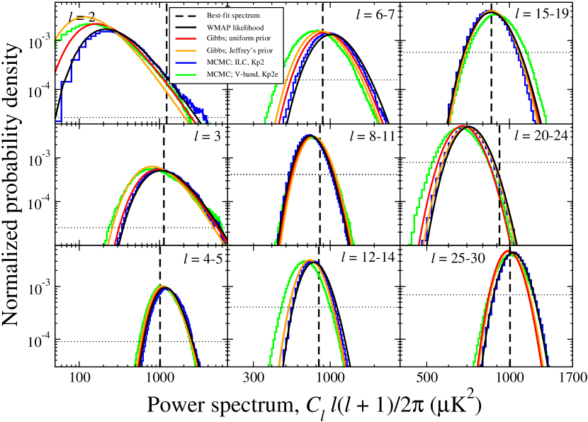
Figure 3.— Posterior distributions (and the WMAP likelihood) computed by different methods and data sets. The colored histograms show the results from MCMC runs with low-$\ell$ likelihood computed in pixel space for different masks, and the black curve shows the Blackwell-Rao estimator computed with V-band/Kp2 Gibbs samples. The vertical dashed lines show the angular power spectrum for the $\Lambda$CDM model that best fits the WMAP data (Hinshaw et al., 2006). The horizontal dashed lines shows the 95% confidence region relative to the Gibbs-based estimate. Note that while the MCMC shows marginalized distributions, the other curves indicate slices through the multi-dimensional distributions with other $C_{\ell}$’s fixed at the best-fit spectrum value.

While the mask explanation can account for some of the discrepancies seen in Figure 1, it only does so at $\ell\leq 12$ where a pixel-based likelihood evaluation is used by the WMAP team. For $\ell>12$ a MASTER-based likelihood is used which is based on the full-resolution template-corrected data. The small discrepancies seen in the range between $12<\ell\lesssim 30$ is therefore due to differences in statistical treatment, and not data selection.

A main question is therefore the following: For what $\ell$-range does the MASTER-based likelihood approximation provide an acceptable fit to the exact likelihood? From Figure 1 it seems clear that $\ell_{\textrm{exact}}\leq 12$ is not sufficient, while $\ell_{\textrm{exact}}\leq 50$ is quite likely more than enough. It is difficult to answer this question based on a power spectrum plot alone, and we will therefore return to this question in Section 6 where we estimate cosmological parameters with various likelihoods.

In order to further illuminate the above issues, we show in Figure 3 a set of different likelihood (and posterior) distributions computed from the WMAP data. The vertical dashed lines show the binned best-fit $\Lambda$CDM spectrum and the curves show the WMAP likelihoods (black), Gibbs + Blackwell-Rao posterior distributions (red/orange) and MCMC posterior distributions (blue/green), respectively. Two sigma confidence regions relative to the Gibbs distributions with uniform priors (red curves) are indicated by horizontal dotted lines.

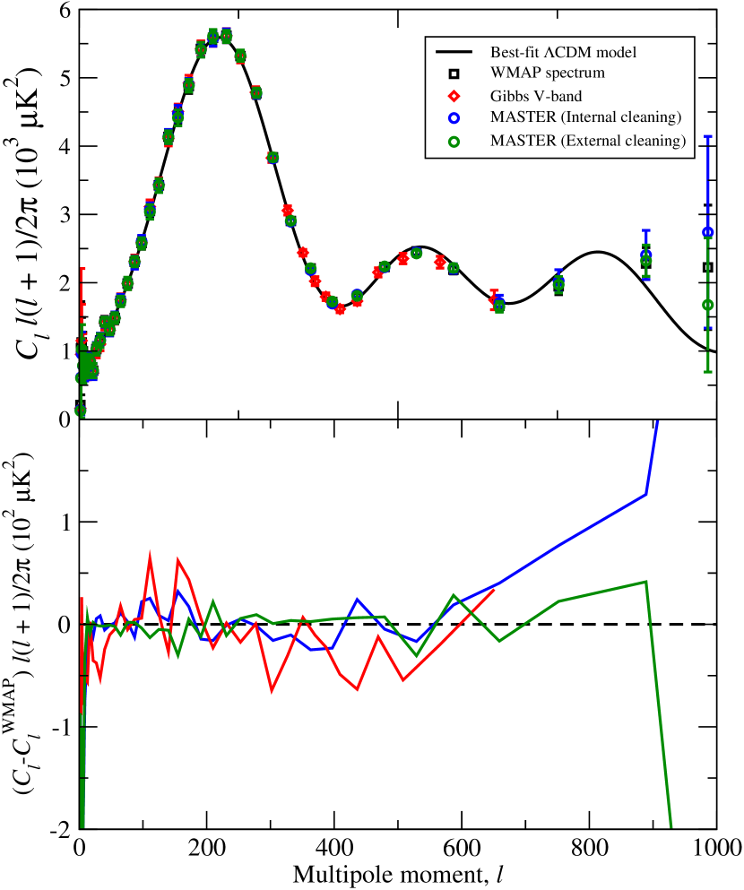
Figure 4.— Top panel: Comparison of power spectra computed from the three-year WMAP data using different techniques and data combinations. Bottom panel: Differences between the spectra computed in this paper and the (appropriately binned) WMAP spectrum.

Many interesting points may be seen in this figure:

1. Comparing the V-band+Kp2e and ILC+Kp2 MCMC runs (green versus blue) we see that the former is shifted systematically to lower values of $C_{\ell}$. This shift is most likely due to a combination of extra fluctuation power coming from the region excluded by Kp2e but included by Kp2, and additional sampling variance from the extended sky cut.

2. The agreement between the ILC+Kp2 MCMC and WMAP likelihood distributions (blue versus black) is generally quite reasonable, but small shifts may be seen in a number of cases, especially for $6\leq\ell\leq 12$. This is likely due to different likelihood regularization (see Appendix A): We use a properly bandwidth limited map within the Nyquist frequency $\ell_{\textrm{N}}=3N_{\textrm{side}}$ but add a small noise term to regularize the covariance matrix; the WMAP code increases $\ell_{\textrm{max}}$ to $4N_{\textrm{side}}$, well beyond the Nyquist frequency, to make the covariance matrix non-singular.

3. The V-band+Kp2e MCMC distributions are generally wider than the ILC+Kp2 distributions (green versus blue) because of a more conservative mask. This is avoided with the full-resolution Gibbs analysis (red curve), since it uses unsmoothed data and thereby does not need to expand the mask. Consequently, the Gibbs distributions are about as wide as the ILC+Kp2 distributions.

4. The Jeffrey’s ignorance prior puts more probability on small values of $C_{\ell}$, but is mostly relevant at very low $\ell$’s (orange versus red). Because of the very large cosmic variance of these multipoles, the effect of the Jeffrey’s prior on cosmological parameters is small.

5. The quadrupole posterior maximum with Jeffrey’s and uniform priors are respectively $105\mu\textrm{K}^{2}$ and $160\mu\textrm{K}^{2}$. Thus, even with Jeffrey’s prior the WMAP quadrupole amplitude is completely unremarkable relative to the best-fit $\Lambda$CDM value, and always well inside the 95% confidence region (vertical dashed versus horizontal dotted lines). The most extreme outlier is that of $20\leq\ell\leq 24$, whose value is low at the $99.4\%$ level.

5. Intermediate- and small-scale analysis

We now consider the intermediate- and small-scale parts of the power spectrum.

5.1. Algorithms and data selection

Since we study full-resolution data in this section, the direct likelihood evaluation techniques are no longer available to us. However, on these scales the MASTER algorithms are applicable, and we once again have multiple methods available for cross-checking purposes. In total four different codes are used, namely Commander (Gibbs sampling; uniform prior), MAGIC (Gibbs sampling; Jeffrey’s prior), MASTERext and MASTERint.

For the Gibbs analyses we consider only the V-band data; the Q-band is considered to be too foreground contaminated for reliable analysis, and the W-band exhibits strong correlated noise that significantly biases any auto-correlation method (Hinshaw et al., 2006). This has been verified in our analyses, and we exclude these bands entirely from the Gibbs analyses. Next, we analyzed the data with both Commander and MAGIC, and obtained identical results (up to convergence) on small and intermediate scales where the prior is less important. Therefore we show only one set of Gibbs results in the following.

In the case of the MASTER analyses, we include cross-spectra only in the final power spectra, and are thus quite safe with respect to correlated noise. For this reason the W-band is included in these cases. Further, for the internal cleaning analysis two different data combinations were considered, namely including either all five bands or only the cleanest Q-, V- and W-bands. The difference between these two spectra was found to be very small. We once again present only one (the five-band) solution here, and note that this solution is not strongly dependent on the low-frequency bands.

The foreground mask is always the full-resolution Kp2 that excludes resolved point sources. Contributions to the power spectrum from unresolved point sources are subtracted band-by-band according to the model described by Hinshaw et al. (2006).

5.2. Results

A summary of our main intermediate- and small-scale power spectra are shown in Figure 4. Four spectra are plotted here: The WMAP spectrum, the Gibbs V-band spectrum, the V+W MASTERext cross-spectrum, and the five-band MASTERint cross-spectrum.

In the top panel we see that the overall agreement is excellent considering the very different approaches taken by the different methods. It is thus very unlikely that algorithmic issues play a dominant role in the determination of cosmological parameters as presented by Spergel et al. (2006) for the small-scale temperature anisotropy results.

In the bottom panel we plot the difference between each of the colored spectra and the WMAP spectrum in order to look for systematic relative trends. Again, we see that the overall agreement is very good, and the only possible anomaly is a slight power deficit for the V-band Gibbs spectrum at $\ell\approx 300$–600. This will be studied further shortly.

The extreme high-$\ell$ discrepancies seen in two MASTER spectra are due to noise weighting differences. For the MASTERext analysis, we obtained the individual cross-spectra from the WMAP team and verified that our spectra are identical to those of the WMAP team. However, while the WMAP spectrum uses an elaborate and nearly maximum-likelihood weighting scheme for co-adding these cross-spectra into one optimal spectrum, we use either simple inverse-variance weighting (for MASTERext) or flat weighting (for MASTERint). Differences in the very low signal-to-noise regime are thus not unexpected.

The excellent agreement seen in Figure 4 is perhaps most remarkable in the case of the MASTERint implementation: While all other spectra more or less correspond to different statistical treatment of the same basic data set, this particular solution takes a drastically different approach, and uses only WMAP data by themselves to correct for foregrounds. Thus, it provides an important and impressive cross-check on the WMAP foreground cleaning approach.

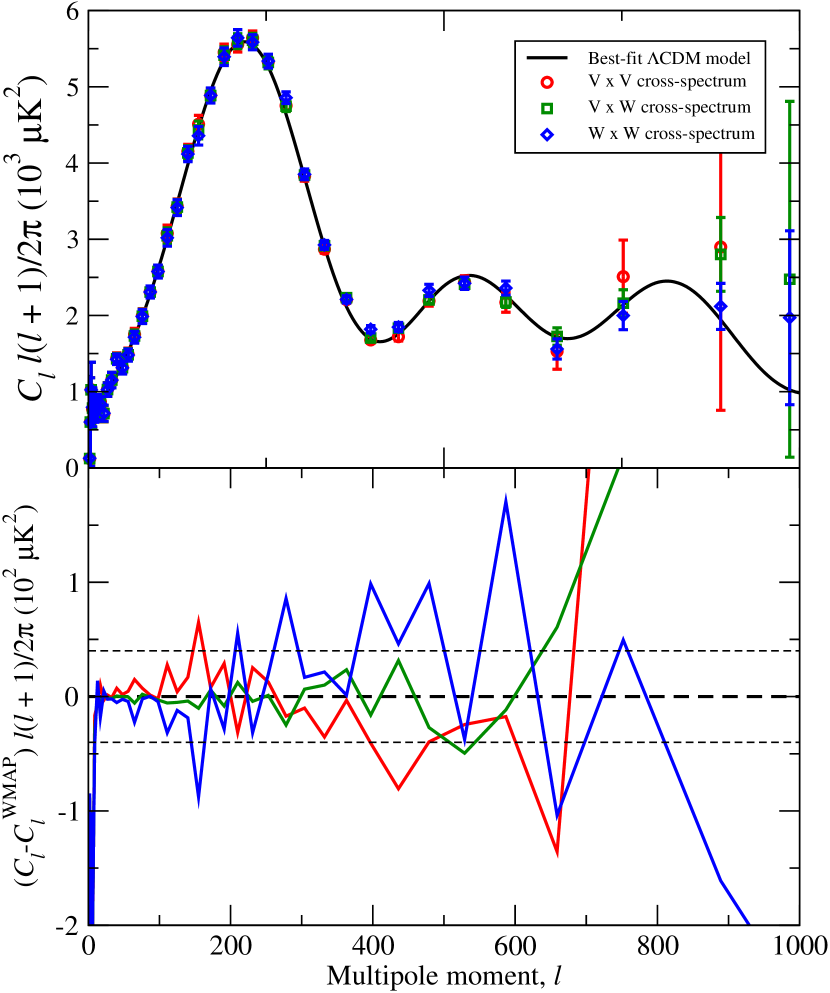
Figure 5.— Power spectrum versus frequency. All spectra are computed from the template-corrected maps with the basic cross-MASTER algorithm. Only the frequency contents vary, as each spectrum only contains cross-information of V$\times$V, V$\times$W and W$\times$W respectively.

However, returning to the power deficit issue seen in the V-band spectrum, we plot in Figure 5 the MASTERext spectra for individual frequency combinations, including V$\times$V, V$\times$W, or W$\times$W spectra, respectively. In this plot we see that the MASTER V-band spectrum agrees very well with the Gibbs V-band spectrum, and lies systematically below the averaged WMAP spectrum between $\ell\approx 300$ and 600. Furthermore, we see that the W-band spectrum lies systematically above the WMAP spectrum in the same range, with a relative bias of up to $80\,\mu\textrm{K}^{2}$. The V$\times$W cross-spectrum lies in between, being more or less an average of the two.

To quantify the significance of this difference, we analyzed the set of 2500 Monte Carlo simulations that was used for the MASTERext analysis. For each simulation we first computed the difference between the W- and V-band spectra, and then the mean (inverse noise variance weighted) difference within some $\ell$-range. Comparing the observed WMAP data to these simulations, we found that the discrepancy is significant at slightly more than $3\sigma$ for both $250\leq\ell\leq 600$ and $400\leq\ell\leq 500$, corresponding to the largest region of asymmetry and to the most discrepant region, respectively. Presumably it is possible to boost the significance by tuning the region further, but on the other hand, the known $\sim 1\%$ beam amplitude uncertainty that is taken into account by the WMAP likelihood code will reduce the signficance by a few tenths of a sigma. Independent of such minor effects, it seems that the probability of this being a statistical fluke is rather small.

After the publication of the present paper, a follow-up study by Huffenberger et al. (2006) revisited the unresolved point source analysis performed by the WMAP team. The main result from that work was a best-fit unresolved point source spectrum amplitude of $A=0.011\,\mu\textrm{K}^{2}\textrm{sr}$ (relative to 41 GHz), which is significantly lower than the value of $A=0.017\,\mu\textrm{K}^{2}\textrm{sr}$ initially reported (Hinshaw et al., 2006) and used in the present paper. Thus, a relatively larger contribution is subtracted from the V-band than from the W-band spectrum, and in effect, the V-band spectrum has been over-corrected. After taking into account this new amplitude, the discrepancy between the two band spectra was found to be significant at $\sim 2\sigma$ using the same test as above.

While the quoted point source correction can account for a substantial amount of the observed discrepancy, there is still a small difference present, and this could possibly indicate further systematics. In this respect, it could be worth considering unmodeled beam asymmetries. As a preliminary step in the three-year analysis, Hinshaw et al. (2006) considered the impact of such asymmetries on the individual cross-spectra. After an extensive analysis, they concluded that their magnitude is less than 1% at $\ell\leq 1000$, and therefore sufficiently small to neglect in further analyses. However, at the relevant scales, the absolute amplitude of the temperature power spectrum is about $2000\,\mu\textrm{K}^{2}$, and a beam asymmetry bias of 1% therefore corresponds to an expected discrepancy of $20\,\mu\textrm{K}^{2}$. This corresponds roughly to $1\sigma$ of the V- versus W-band difference, and, if determined appropriate, its correction could bring the overall difference well within the statistical errors. Fortunately, this issue will be clearer with additional years of WMAP observations.

6. Cosmological parameters

In the previous two sections we considered the temperature angular power spectrum as observed by WMAP, and our main conclusion from these analyses is that the WMAP spectrum is reasonable at all angular scales. However, there are small but clearly noticeable biases at both large and small scales. In this section, we seek to quantify the impact of this bias in terms of the cosmological parameters for a minimal six-parameter $\Lambda$CDM model. The combined effect of both the low- and high-$\ell$ discrepancies are studied by Huffenberger et al. (2006), and the effect on extended cosmological models (e.g., models including massive neutrinos and running of the spectral index) are considered by Kristiansen et al. (2006).

Table 1Cosmological parameters

		WMAP + BR	WMAP + BR	WMAP + Pixel	Shift
Parameter	WMAP	($\ell_{\textrm{max}}=12$)	($\ell_{\textrm{max}}=30$)	($\ell_{\textrm{max}}=30$)	(in $\sigma_{\textrm{WMAP}}$)
WMAP data only
$\Omega_{\textrm{b}}\,h^{2}$	$0.0222\pm 0.0007$	$0.0222\pm 0.0007$	$0.0224\pm 0.0007$	$0.0224\pm 0.0007$	-0.3
$\Omega_{\textrm{m}}$	$0.241\pm 0.036$	$0.241\pm 0.0037$	$0.230\pm 0.033$	$0.234\pm 0.035$	string0.3
$\log(10^{10}A_{\textrm{s}})$	$3.019\pm 0.067$	$3.017\pm 0.068$	$3.014\pm 0.068$	$3.013\pm 0.068$	string0.1
$h$	$0.731\pm 0.033$	$0.731\pm 0.032$	$0.743\pm 0.033$	$0.739\pm 0.033$	-0.4
$n_{\textrm{s}}$	$0.954\pm 0.016$	$0.955\pm 0.016$	$0.961\pm 0.016$	$0.960\pm 0.017$	-0.4
$\tau$	$0.090\pm 0.030$	$0.088\pm 0.030$	$0.090\pm 0.030$	$0.088\pm 0.030$	string0.0
WMAP + Acbar + BOOMERanG
$\Omega_{\textrm{b}}\,h^{2}$	$0.0225\pm 0.0007$	$0.0225\pm 0.0007$	$0.0227\pm 0.0007$	$0.0227\pm 0.0007$	-0.3
$\Omega_{\textrm{m}}$	$0.239\pm 0.031$	$0.240\pm 0.032$	$0.229\pm 0.030$	$0.233\pm 0.031$	string0.3
$\log(10^{10}A_{\textrm{s}})$	$3.030\pm 0.064$	$3.028\pm 0.065$	$3.025\pm 0.066$	$3.023\pm 0.0065$	string0.1
$h$	$0.737\pm 0.029$	$0.736\pm 0.031$	$0.749\pm 0.031$	$0.744\pm 0.031$	-0.4
$n_{\textrm{s}}$	$0.958\pm 0.016$	$0.959\pm 0.016$	$0.965\pm 0.016$	$0.964\pm 0.016$	-0.4
$\tau$	$0.091\pm 0.030$	$0.090\pm 0.030$	$0.091\pm 0.030$	$0.089\pm 0.030$	stringstring0.0

Note. — Comparison of marginalized parameter results obtained from the WMAP likelihood (second column), the WMAP + Blackwell-Rao hybrid (third and fourth columns), and from the WMAP + $N_{\textrm{side}}=16$ pixel-based likelihood (fifth column). The latter three were based on the template-corrected V-band data at low $\ell$’s. The relative shift between the WMAP and the $\ell_{\textrm{max}}=30$ BR hybrid (in units of $\sigma_{\textrm{WMAP}}$) is shown in the rightmost column.

We perform four sets of similar analyses, all primarily based on the WMAP likelihood code. First, we adopt the WMAP likelihood as provided. Second, we replace the low-$\ell$ likelihood (both the pixel-based estimator and the low-$\ell$ MASTER estimator) with a Blackwell-Rao (BR) Gibbs-based estimator for $\ell\leq 30$ (Chu et al., 2005). Third, we do the same for $\ell\leq 12$ alone. Finally, we use the $N_{\textrm{side}}=16$, $\ell_{\textrm{max}}=30$ pixel-based likelihood for the V-band and Kp2e cut described earlier. For all cases, we analyze two data combinations; the WMAP data alone, and the combination of WMAP, Acbar (Kuo et al., 2004) and BOOMERanG (Montroy et al., 2005; Piacentini et al., 2005; Jones et al., 2005). Marginalization of SZ was not included.

Figure 6.— Probability contours for a simple amplitude/tilt model ($C_{\ell}(q,n)=q\,C_{\ell}^{\textrm{fid}}\left(\ell/10\right)^{n}$, $C_{\ell}^{\textrm{fid}}$ being the best-fit $\Lambda$CMB model) fitted to the WMAP likelihood (solid lines) and to the Gibbs sampled posterior (dotted lines). Contours indicate 68 and 95% confidence regions. Note the shift to higher amplitudes for the WMAP results, and also that the Gibbs results are more closely centered on $(q,n)=(1,0)$.

Note that we use the WMAP likelihood at high $\ell$’s in all cases in order to highlight the effects of the low-$\ell$ likelihood bias. While using a Gibbs sampling based estimator even at high $\ell$’s could potentially have beneficial effects in terms of uncertainties, it might confuse the low-$\ell$ bias analysis by introducing other differences.

The cosmological parameters corresponding to these likelihoods were established through standard Markov Chain Monte Carlo analysis. In keeping with our philosophy of cross-verification, two independent codes were used for a few cases. In the first case, CosmoMC (Lewis & Bridle, 2002) was downloaded and appropriately modified, and in the second, a stand-alone code was written from scratch in C++. The two codes returned identical distributions, and as usual we show only one set of results in the following. We also performed similar analyses using only temperature-data, imposing a Gaussian prior on the optical depth of $\tau=0.10\pm 0.03$ to simulate the effect of polarization data, but without relying on the accuracy of these. As expected, we then obtained very similar results to those reported here.

Before reporting the physical parameters, we consider a very simple phenomenological model in order to gain intuition on what to expect. Specifically, we fit a model with a free amplitude and tilt to both the WMAP likelihood and the WMAP+BR $\ell_{\textrm{max}}=30$ hybrid,

$$C_{\ell}(q,n)=q\,C_{\ell}^{\textrm{fid}}\left(\frac{\ell}{10}\right)^{n}.$$ (2)

Here $C_{\ell}^{\textrm{fid}}$ is a fiducial model (chosen to be the best-fit $\Lambda$CDM power law model), $q$ is a relative amplitude, and $n$ is a tilt parameter. Since we expect the fiducial model to be a good fit to the data, we anticipate values of $(q,n)$ around $(1,0)$. In this exercise we include only data between $2\leq\ell\leq 20$. The results from these computations are shown in Figure 6, where contours indicate 68 and 95% confidence regions. WMAP results are indicated by solid lines and Blackwell-Rao results by dotted lines.

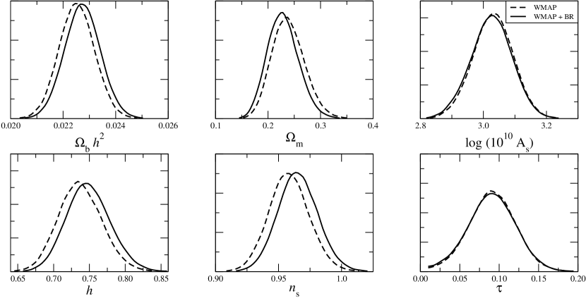
Figure 7.— Comparison of marginal probability distributions as computed with the WMAP likelihood (dashed) and with the WMAP + Blackwell-Rao hybrid (solid) at $2\leq\ell\leq 30$. The results are based on the WMAP, Acbar and BOOMERanG data, as described in the text.

By far the most striking feature is a $\sim 0.5\sigma$ shift in amplitude towards lower values for our revised posterior, consistent with the low-$\ell$ power spectrum results shown earlier. However, it is interesting to notice that the Blackwell-Rao contours are more centered on $(q,n)=(1,0)$ than the WMAP contours: This indicates that there is less tension between the low-$\ell$ and high-$\ell$ parts of the spectrum when using our approach instead of the WMAP approach.

For the physical parameter estimation, we adopted a standard six-parameter $\Lambda$CDM model with $\{\Omega_{\textrm{b}}h^{2},\Omega_{\textrm{c}}h^{2},\theta,\tau,n_{\textrm{s}},\log(10^{10}A_{\textrm{s}})\}$ as our free parameters. The priors were chosen to be uniform for all parameters.

The results from these computations are summarized in Table 1 and Figure 7, and a number of interesting points may be seen here. First, comparing the WMAP likelihood to the $\ell\leq 12$ WMAP + BR hybrid (second and third columns of Table 1), we see that the small change due to mask expansion at $\ell\leq 12$ seen in Figure 2 has no impact in terms of cosmological parameters. In effect, the cosmic variance on these very large scales hides such problems.

However, comparing the WMAP likelihood to the $\ell\leq 30$ WMAP + BR hybrid (second and fourth columns), a different picture is seen. In this case, we find shifts of up to $0.4\sigma$ for both $h$ and $n_{\textrm{s}}$ (right column). Thus, the MASTER-based approximation used in this regime appears to be inadequate for the precision required by the WMAP data. That the differences are indeed due to statistical treatment is confirmed by the results for the low-$\ell$ pixel-based hybrid, which extends the original WMAP analysis simply by using direct evaluation up to $\ell=30$ instead of $\ell=12$.

We also performed a second analysis with the WMAP + BR hybrid, this time making the transition at $\ell=50$. Fortunately, the results from these computations were essentially identical to those for $\ell=30$, and this implies that a pixel-based likelihood for $N_{\textrm{side}}=16$ may still be used for the precision of the WMAP data. However, the computational expense of this approach is already pushing close to what is reasonable, and currently dominates the MCMC cost. This illustrates very well the advantages of the Gibbs sampling approach, in which identical results are obtained at only a fraction of the computational cost.

In Figure 7, we compare the results for the WMAP likelihood and WMAP + BR hybrid likelihood from the combined WMAP, Acbar and BOOMERanG analysis in terms of marginalized probability distributions. With a few exceptions, the low-$\ell$ bias results in a shift of a few tenths of a sigma. Perhaps most interesting is the effect on the much debated $n_{\textrm{s}}$: This distribution is shifted towards higher values by the new low-$\ell$ likelihood, and the evidence for $n_{\textrm{s}}\neq 1$ is thus reduced.

Finally, we note that with Planck’s reach to higher $\ell$’s, the $2\leq\ell\lesssim 30$ data will not be critically important for constraining $n_{\textrm{s}}$; removing $\ell\leq 30$ will increase $\sigma(n_{\textrm{s}})$ by less than 10%. Planck’s constraints on $n_{\textrm{s}}$ will thus not be dependent on low-$\ell$ polarization measurements, and therefore less sensitive to residual foregrounds.

To summarize, we find that the improvements we make to the low-$\ell$ likelihood have a small but noticeable impact on the cosmological parameters reported by Spergel et al. (2006). In particular, the evidence for $n_{\textrm{s}}\neq 1$ is weakened by $0.4\sigma$, which is significant given the initial marginal $\sim 2.5-3\sigma$ detection. For full details on results correcting for both this low-$\ell$ statistical issue and the high-$\ell$ point source issue, we refer to Huffenberger et al. (2006) and Kristiansen et al. (2006).

7. Conclusions

In this paper we have made an extensive re-analysis of the WMAP temperature anisotropy data. We have re-computed the power spectrum using six different codes, and the cosmological parameters with two different codes. Five different groups have contributed with separate computations. In total, the amount of cross-checks provided by this effort leads us to conclude that most important analysis issues concerning the three-year temperature power spectrum are well understood.

Our main conclusion from this work is that we confirm the WMAP temperature power spectrum on most scales. However, subtle discrepancies are found both at large and small scales, and these can be summarized as follows:

1. There is a small but significant bias at large angular scales (5–10% at $\ell\leq 30$) in the WMAP power spectrum and published likelihood code. This is primarily due to statistical issues in the form of an inadequate likelihood approximation, and secondarily due to residual foregrounds.

2. There is a systematic bias between the V- and W-bands. This has recently been identified by Huffenberger et al. (2006) to be at least partially caused by over-correction of unresolved point sources. However, even after correcting for this, a small discrepancy is present, and this could possibly indicate further systematics. A possible candidate worth considering could be uncorrected beam asymmetries.

3. The low-$\ell$ likelihood bias has a noticable effect of some parameters. Most interestingly, it increases $n_{\textrm{s}}$ by $0.4\sigma$, reducing the nominal detection of $n_{\textrm{s}}\neq 1$ from $\sim 2.7$ to $\sim 2.3\sigma$. Further, as reported by Huffenberger et al. (2006), correcting for the point source over-correction increases $n_{\textrm{s}}$ by an additional $\sim 0.3\sigma$, to a final significance of $n_{\textrm{s}}\neq 1$ of $\sim 2.0$.

In addition to these cosmologically important results, we make a few algorithmic recommendations based on the work presented here regarding the WMAP analysis. First and foremost, an exact likelihood evaluation should be used at least up to $\ell\leq 30$. Either direct evaluation or Gibbs sampling can be used for these scales, but of course, the negligible computational cost of the latter, when incorporated into an MCMC sampler, makes it the preferred choice. Second, we advocate using the more conservative Kp2e cut at very low l as a hedge against possible foreground contamination just outside the directly downgraded Kp2 mask. However, this has a negligible effect in terms of cosmological parameters.

The products from the Gibbs sampling analysis (with a uniform prior) are made publically available in the form of three data sets. First, the most relevant for the applications presented in this paper is the collection of $4\times 1000$ sky signal spectrum samples. These form the basis of the Blackwell-Rao estimator, and may be used for parameter estimation as demonstrated in this paper. A corresponding Fortran 90 module is also provided. Second, a set of 4000 ensemble averaged spectrum samples are presented. These may be used for visualization purposes of the power spectrum. Third, a set of sky map samples are provided for $\ell\leq 50$. These may be used for analyses that require phase information, for instance studies of non-Gaussianity.

Thus, we conclude that although fast methods such as MASTER are very useful in the early stages of analyzing a new experiment, when fast turn around times are essential, the extensions to Gibbs sampling (as described in the Appendices) have now rendered an exact method quite tractable with currently available computing resources. Based upon our experience with these methods, we believe that Gibbs sampling can and will play a significant role in the future analysis of Planck data.

Appendix A A. Low-$\ell$ likelihood evaluation

Low-$\ell$ likelihood evaluation from high-resolution data has received considerable attention in the last few years (Efstathiou, 2004; Slosar et al., 2004; Hinshaw et al., 2006). The reason is simply that while the currently popular pseudo-spectrum power spectrum estimators (Hivon et al., 2002) work very well on intermediate and small angular scales, they are clearly sub-optimal on large scales.

The log-likelihood for a pixelized Gaussian random field $\mathbf{d}$, with vanishing mean and covariance matrix $\mathbf{C}$, is given by

$$-2\log\mathcal{L}=\mathbf{d}^{t}\mathbf{C}^{-1}\mathbf{d}+\log|\mathbf{C}|,$$ (A1)

up to a normalization constant. Evaluation of this expression requires inversion of the pixel-pixel covariance matrix, and therefore scales as $\mathcal{O}(N_{\textrm{pix}}^{3})$. Consequently, direct likelihood analysis of mega-pixel maps is not currently feasible.

The covariance matrix consists of a series of terms depending on the data model, but at the very least one needs a signal term $\mathbf{S}$, which for an assumed isotropic CMB is given by the angular power spectrum $C_{\ell}$,

$$S_{ij}=\frac{1}{4\pi}\sum_{\ell=2}^{\ell_{\textrm{max}}}(2\ell+1)C_{\ell}b_{\ell}^{2}P_{\ell}(\cos\theta_{ij}).$$ (A2)

Here $b_{\ell}$ is the Legendre transform of the (circularly symmetric) experimental beam, $P_{\ell}(x)$ are the Legendre polynomials, $\theta_{ij}$ is the angle between pixels $i$ and $j$, and $\ell_{\textrm{max}}$ is a sufficiently large multipole. The exact definition of “sufficiently large” will be made explicit shortly.

Next, in most real-world applications there is also a term describing instrumental noise, $\mathbf{N}$. Often, this is modeled as independent between pixels (white), and given by an overall noise level per observation $\sigma_{0}$ and a total number of observations per pixel $N_{\textrm{obs}}(i)$, such that $N_{ij}=\sigma_{0}/\sqrt{N_{\textrm{obs}}(i)}\delta_{ij}$. For current CMB experiments, such as WMAP, this is strongly sub-dominant to the signal term on large angular scales, and may in principle be omitted without significant loss of accuracy. However, this is not entirely true, since it can (and should) play an important role in regularizing the covariance matrix.

Finally, it is useful to include a number of template terms over which amplitudes one wishes to marginalize (Bond et al., 1998; Slosar et al., 2004). Consider for instance a given foreground template $\mathbf{f}$ whose spatial structure is known, but overall amplitude is unknown. Then the corresponding covariance matrix is given by the outer product $\mathbf{F}=\mathbf{f}\,\mathbf{f}^{t}$, and by assigning a sufficiently large uncertainty to this structure the corresponding mode is projected out from the data. In total, the covariance matrix may be written as

$$\mathbf{C}=\mathbf{S}+\mathbf{N}+\sum_{i}\lambda_{i}\mathbf{F}_{i},$$ (A3)

where $\lambda_{i}$ are numerically sufficiently large constants.

Conceptually speaking, the above description completely defines the likelihood problem. However, for the particular problem of low-resolution analysis with high signal-to-noise data there is one particular issue that must be considered in greater detail in order to produce robust results, and that is the relationship between a finite pixelization, bandwidth limitation, and covariance matrix regularization.

For the expansion in equation A2 to be valid, $\ell_{\textrm{max}}$ must be chosen sufficiently large such that there is negligible power beyond this multipole. At the same time it must be smaller than the corresponding Nyquist frequency of the chosen pixelization. For HEALPix the recommended upper limit on this value is $\ell_{\textrm{max}}=2\,N_{\textrm{side}}$ (where $N_{\textrm{pix}}=12N_{\textrm{side}}^{2}$), but through various numerical techniques it can be pushed to $\ell_{\textrm{max}}=3\,N_{\textrm{side}}$. Beyond this, one is almost assured to get nonsensical results, and one must therefore make sure that the experimental beam suppresses all signal beyond this value. (A good rule-of-thumb is that the beam FWHM must be at least 2.5 times the pixel size. For example, at $N_{\textrm{side}}=16$ the pixel size is $3.6^{\circ}$, and the smallest beam supported by this pixelization is $9^{\circ}$ FWHM.)

In a pure signal map $\mathbf{s}$, with a given bandwidth limit $\ell_{\textrm{max}}$, there are $(\ell_{\textrm{max}}+1)^{2}$ real modes. Enforcing the recommended Nyquist limit of $\ell_{\textrm{max}}=2\,N_{\textrm{side}}$, a given pixelization can thus maximally resolve $\sim 4\,N_{\textrm{side}}^{2}$ independent modes, which is considerably less than the number of pixels in the map, $N_{\textrm{pix}}=12N_{\textrm{side}}^{2}$. By a simple mode counting argument, it is clear that a signal-only covariance matrix necessarily will be singular, and consequently, it must be regularized in some way before inversion.

The solution used by the currently available WMAP likelihood code is simply to increase $\ell_{\textrm{max}}$ to $4\,N_{\textrm{side}}$, and thereby go beyond the Nyquist frequency of the pixelization. While it is true that this does indeed make the matrix invertible (since the number of projected modes is now greater than the number of pixels), it is also mathematically arbitrary, highly pixelization dependent, and not connected to the observed data.

A much more reliable approach is readily available by means of the noise covariance matrix. By adding a small amount of white noise to the data, which has $N_{\textrm{pix}}$ independent modes, the matrix becomes invertible, and the data description is still accurate. A stable and well defined algorithm for computing low-resolution likelihoods from high-resolution data may be formulated as follows:

1. Choose some $\ell_{\textrm{max}}$ of interest.

2. Determine the smallest pixelization that comfortably supports this scale and the corresponding pixel size $\theta_{\textrm{pix}}$.

3. Smooth the data with a Gaussian beam of $2.5\theta_{\textrm{pix}}$ FWHM.

4. Add Gaussian noise to the data with a variance such that the data are strongly noise dominated at $3N_{\textrm{side}}$.

5. Compute the likelihood as described above, with appropriately defined covariance matrices.

Appendix B B. Some Gibbs sampling extensions

Power spectrum estimation through Gibbs sampling was originally introduced to CMB applications by Jewell et al. (2004) and Wandelt et al. (2004), and later implemented for high-resolution applications like WMAP by Eriksen et al. (2004) and O’Dwyer et al. (2004). The codes we use in the present paper are direct descendants from those described in the latter two papers, but with a few simple extensions we describe in this Appendix. Specifically, in order to reduce the Markov chain correlation length in the low signal-to-noise regime, we have implemented binned $C_{\ell}$ sampling and sub-space sampling, and also sampling with Jeffrey’s ignorance prior which has an effect on large angular scales.

Let us first recall the basic idea of Gibbs sampling. Suppose we want to draw samples from a complicated joint probability distribution $P(x,y)$, but only know how to sample from the conditional distributions $P(x|y)$ and $P(y|x)$. Then the theory of Gibbs sampling tells us that joint samples $(x^{i},y^{i})$ may be obtained by alternately drawing from these two distributions, $x^{i+1}\leftarrow P(x|y^{i})$ and $y^{i+1}\leftarrow P(y|x^{i+1})$. As shown by Jewell et al. (2004) and Wandelt et al. (2004), this may be applied to CMB analysis because it is in fact feasible to sample from both $P(C_{\ell}|\mathbf{d},\mathbf{s})$ and $P(\mathbf{s}|\mathbf{d},C_{\ell})$ where $\mathbf{d}$ are observed data and $\mathbf{s}$ is the true CMB sky. Explicitly, the algorithm may be described by these two steps:

$$\mathbf{s}^{i+1} \leftarrow P(\mathbf{s}|C_{\ell}^{i},\mathbf{d}),$$ (B1)

$$C_{\ell}^{i+1} \leftarrow P(C_{\ell}|\mathbf{s}^{i+1}).$$ (B2)

Here $\leftarrow$ indicates sampling from the distribution on the right. Thus, after some burn-in time $(C_{\ell}^{i},\mathbf{s}^{i})$ will be drawn from the desired distribution, and these samples may subsequently be used to establish marginal $P(C_{\ell}|\mathbf{d})$ and $P(\mathbf{s}|\mathbf{d})$ if desired.

B.1. Binned $C_{\ell}$ sampling

One of the major problems with the implementations described by Eriksen et al. (2004) was their inability to probe the low signal-to-noise regime. The reason was simply that the Markov chain step size between two consecutive $C_{\ell}$ samples is given by cosmic variance alone, while the full posterior is given by both cosmic variance and noise. Thus, in order to move a significant distance in the high-$\ell$ regime, a very large number of steps is required.

One way to improve on this situation is simply to bin the power spectrum, and thereby increase the signal-to-noise ratio per sampled parameter. (Note that such binning must be done internally in the $P(C_{\ell}|\mathbf{d},\mathbf{s})\equiv P(C_{\ell}|\mathbf{s})$ sampler in order to earn an improvement – binning by post-processing does not have the same effect.)

Before describing the binned sampling algorithm, it is useful to recall the single-$\ell$ algorithm for sampling from $P(C_{\ell}|\mathbf{s})$: First compute the power spectrum of the signal map, and write it for convenience on the form $\sigma_{\ell}=\sum_{m=-\ell}^{\ell}|a_{\ell m}|^{2}$. Next, draw $2\ell-1$ Gaussian random variates $\rho_{\ell}^{j}$ with zero mean and unit variance, and form the sum $\rho_{\ell}^{2}=\sum_{j=1}^{2\ell-1}|\rho_{\ell}^{j}|^{2}$. Then the desired power spectrum sample is given by

$$C_{\ell}^{i+1}=\frac{\sigma_{\ell}}{\rho_{\ell}^{2}}$$ (B3)

Sampling binned $C_{\ell}$’s is very similar. First, we define the binning scheme to be uniform in $C_{\ell}\,\ell(\ell+1)$, and choose some bin limits $\ell_{\textrm{min}}$ and $\ell_{\textrm{max}}$. We then form the quantity

$$\sigma_{\textrm{b}}=\sum_{\ell=\ell_{\textrm{min}}}^{\ell_{\textrm{max}}}\sum_{m=-\ell}^{\ell}\ell(\ell+1)\,|a_{\ell m}|^{2}.$$ (B4)

The number of independent harmonic modes in this sum is $n\equiv(\ell_{\textrm{max}}+1)^{2}-\ell_{\textrm{min}}^{2}$, and therefore we draw $n$ Gaussian random variates $\rho^{j}$ with zero mean and unit variance. Next, we form the sum

$$\rho_{\textrm{b}}^{2}=\sum_{j=1}^{n}|\rho^{j}|^{2}.$$ (B5)

The common bin sample value is then

$$C_{\textrm{b}}=\frac{\sigma_{\textrm{b}}}{\rho_{\textrm{b}}},$$ (B6)

and the actual power spectrum sample coefficients are

$$C_{\ell}=C_{\textrm{b}}/\ell(\ell+1).$$ (B7)

B.2. Sub-space sampling

A second technique to speed up convergence is sub-space sampling. As described above, Gibbs sampling simply means sampling one parameter at a time while conditioning on all others. If beneficial, we may therefore choose to sample only a few $C_{\ell}$’s and $\sigma_{\ell}$’s at a time while conditioning on all others.

Specifically, we may extend the basic sampling scheme given in Equation B2 as follows.

$$\mathbf{s}_{\textrm{low}}^{i+1} \leftarrow P(\mathbf{s}_{\textrm{low}}|C_{\ell,\textrm{low}}^{i},C_{\ell,\textrm{high}}^{i},\mathbf{s}^{i}_{\textrm{high}},\mathbf{d}),$$ (B8)

$$C_{\ell,\textrm{low}}^{i+1} \leftarrow P(C_{\ell,\textrm{low}}|\mathbf{s}^{i+1}_{\textrm{low}}),$$ (B9)

$$\mathbf{s}_{\textrm{high}}^{i+1} \leftarrow P(\mathbf{s}_{\textrm{high}}|C_{\ell,\textrm{high}}^{i},C_{\ell,\textrm{low}}^{i},\mathbf{s}^{i+1}_{\textrm{low}},\mathbf{d}),$$ (B10)

$$C_{\ell,\textrm{high}}^{i+1} \leftarrow P(C_{\ell,\textrm{high}}|\mathbf{s}^{i+1}_{\textrm{high}}).$$ (B11)

Sampling from $P(C_{\ell}|\mathbf{s})$ for a sub-set follows exactly the same algorithm as before. For $P(\mathbf{s}_{\textrm{low}}|C_{\ell},\mathbf{s}_{\textrm{high}},\mathbf{d})$ two trivial modifications must be made: The complementary sky signal that is conditioned upon must be subtracted from the data prior to sampling, and the corresponding $C_{\ell}$ coefficients must be set to zero.

The advantage of this partitioning lies in the relationship between pre-conditioning performance and correlation length: The Markov chain correlation length is very short in the high signal-to-noise regime but very long in the low signal-to-noise regime. Thus, in principle we would like to make a larger number of steps at high $\ell$’s than at low $\ell$’s, in order to obtain similar mixing properties everywhere. On the other hand, most of the computational expense for Gibbs sampling is spent on sampling from $P(\mathbf{s}|C_{\ell},\mathbf{d})$ for which a linear system must be solved using Conjugate Gradients. This linear system is dense in the high signal-to-noise regime, but nearly diagonal in the low signal-to-noise regime. Therefore, by conditioning on the computationally expensive high signal-to-noise components, we can sample the high-$\ell$ components more aggressively with a low computational cost per sample.

For the analysis presented here, this is implemented through the following sampling scheme:

• For each main sample stored on disk,

  • draw one all-scale sample ($\sim 120$ CG iterations).

  • draw three intermediate-scale ($\ell\geq 300$) samples ($\sim 20$ CG iterations).

    • draw three small-scale ($\ell\geq 400$) samples ($\sim 7$ CG iterations) for each intermediate-scale sample.

The pre-conditioner may be individually tuned to each case. In particular, an expensive pre-conditioner is used for the first case, and a cheap, diagonal pre-conditioner is used for the latter two. Also, if for a particular application one finds that convergence is slow for low $\ell$’s (such as foreground sampling), one may condition on, say, $\ell>50$ and solve the system exactly in one single iteration using the pre-conditioner described by Eriksen et al. (2004).

To summarize, it is straightforward to obtain good convergence even in the low signal-to-noise regime using Gibbs sampling with the introduction of binned $C_{\ell}$ sampling and sub-space sampling. For the V-band analyses presented in this paper ($N_{\textrm{side}}=512$, $\ell_{\textrm{max}}=700$), we produced 4000 such de-correlated samples in three days with 16 processors, reaching a Gelman-Rubin statistic value of $R-1<0.05$ for the last bin and $R-1<0.01$ for $\ell<600$.

B.3. Jeffrey’s prior

The Bayesian approaches to power spectrum estimation require an explicit statement of the prior probability distribution of the power spectrum. This prior reflects the experimenter’s knowledge, or lack thereof, about the power spectrum before the data are collected.

The Jeffreys prior is often useful because it encodes a complete lack of knowledge about scale. If we have some parameter, such as a value of $C_{\ell}$, which we know is positive, but have no idea of its order of magnitude, then we can use $P(C_{\ell})=1/C_{\ell}$ as our prior. This is the Jeffreys prior, and it gives equal weight to each logarithmic bin, reflecting the initial belief that $C_{\ell}$ is equally likely to be in any of them.

In practice, the scale of the parameter in question is not completely unknown. In the case of the CMB, for example, $\sqrt{C_{\ell}}<2.7\mbox{K}$, since the temperature of the CMB cannot be negative anywhere on the sky. While this information should technically be included in the prior, it is often not necessary to include it. In this case, the data already constrain the values of $C_{\ell}$ so strongly that the above cutoff in the prior would have no effect on the final posterior distribution.

The Jeffreys prior weights the posterior probability more toward low values of $C_{\ell}$ than a uniform prior would. The uniform prior ($P(C_{\ell})=\mbox{constant}$) is useful because the posterior is then exactly equal to the likelihood. We plot the posterior with both priors in figure 4, to show the effect of the Jeffreys prior in the final posterior distribution.

References

- Bennett et al. (2003a) Bennett, C. L. et al. 2003a, ApJS, 148, 1
- Bennett et al. (2003b) Bennett, C. L., et al. 2003b, ApJS, 148, 97
- Bond et al. (1998) Bond, J. R., Jaffe, A. H., & Knox, L. 1998, Phys. Rev. D, 57, 2117
- Chu et al. (2005) Chu, M., Eriksen, H. K., Knox, L., Górski, K. M., Jewell, J. B., Larson, D. L., O’Dwyer, I. J., & Wandelt, B. D. 2005, Phys. Rev. D, 71, 103002
- Cole et al. (2005) Cole, S., et al. 2005, MNRAS, 362, 505
- Efstathiou (2004) Efstathiou, G. 2004, MNRAS, 348, 885
- Eriksen et al. (2004) Eriksen, H. K., et al. 2004, ApJS, 155, 227
- Eriksen et al. (2006) Eriksen, H. K., et al. 2006, ApJ, 641, 665
- Finkbeiner et al. (1999) Finkbeiner D.P., Davis M., & Schlegel D.J. 1999, ApJ, 524, 867
- Finkbeiner (2003) Finkbeiner, D. P. 2003, ApJS, 146, 407
- Fosalba & Szapudi (2004) Fosalba, P., & Szapudi, I. 2004, ApJ, 617, L95
- Gorski et al. (1996) Górski, K. M., Banday, A. J., Bennett, C. L., Hinshaw, G., Kogut, A., Smoot, G. F., & Wright, E. L. 1996, ApJ, 464, L11
- Górski et al. (2005) Górski, K. M., Hivon, E., Banday, A. J., Wandelt, B. D., Hansen, F. K., Reinecke, M., & Bartelmann, M. 2005, ApJ, 622, 759
- Hinshaw et al. (2003) Hinshaw, G., et al. 2003, ApJS, 148, 135
- Hinshaw et al. (2006) Hinshaw, G., et al. 2006, ApJ, submitted [astro-ph/0603451]
- Hivon et al. (2002) Hivon, E., Górski, K. M., Netterfield, C. B., Crill, B. P., Prunet, S., & Hansen, F. 2002, ApJ, 567, 2
- Huffenberger et al. (2006) Huffenberger, K. M., Eriksen, H. K., & Hansen, F. K. 2006, ApJ, submitted, [astro-ph/0606538]
- Jewell et al. (2004) Jewell, J., Levin, S., & Anderson, C. H. 2004, ApJ, 609, 1
- Jones et al. (2005) Jones, W. C., et al. 2005, ApJ, submitted, [astro-ph/0507494]
- Knox et al. (2001) Knox, L., Christensen, N., & Skordis, C. 2001, ApJ, 563, L95
- Kuo et al. (2004) Kuo, C. L., et al. 2004, ApJ, 600, 32
- Kristiansen et al. (2006) Kristiansen, J. R., Elgarœy, Œ., & Eriksen, H. K. 2006, Phys. Rev. D, submitted [astro-ph/0608017]
- Lewis & Bridle (2002) Lewis, A., & Bridle, S. 2002, Phys. Rev. D, 66, 103511
- Montroy et al. (2005) Montroy, T. E., et al. 2005, ApJ, submitted, [astro-ph/0507514]
- O’Dwyer et al. (2004) O’Dwyer, I. J. et al. ApJ, 617, L99
- Page et al. (2006) Page, L., et al. 2006, ApJ, submitted, [astro-ph/0603450]
- Piacentini et al. (2005) Piacentini, F, et al. 2005, ApJ, submitted [astro-ph/0507507]
- Saha et al. (2006) Saha, R., Jain, P., & Souradeep, T. 2006, ApJL, 645, L89
- Slosar et al. (2004) Slosar, A., Seljak, U., & Makarov, A. 2004, Phys. Rev. D, 69, 123003
- Spergel et al. (2006) Spergel, D. N., et al. 2006, ApJ, submitted, [astro-ph/0603449]
- Tegmark et al. (2003) Tegmark, M., de Oliveira-Costa, A., & Hamilton, A. J. 2003, Phys. Rev. D, 68, 123523
- Wandelt et al. (2004) Wandelt, B. D., Larson, D. L., & Lakshminarayanan, A. 2004, Phys. Rev. D, 70, 083511