Cosmology and Astrophysical Constraints of Gauss-Bonnet Dark Energy

Abstract

Cosmological consequences of a string-motivated dark energy scenario featuring a scalar field coupled to the Gauss-Bonnet invariant are investigated. We study the evolution of the universe in such a model, identifying its key properties. The evolution of the homogeneous background and cosmological perturbations, both at large and small scales, are calculated. The impact of the coupling on galaxy distributions and the cosmic microwave background is examined. We find the coupling provides a mechanism to viably onset the late acceleration, to alleviate the coincidence problem, and furthermore to effectively cross the phantom divide at the present while avoiding a Big Rip in the future. We show the model could explain the present cosmological observations, and discuss how various astrophysical and cosmological data, from the Solar system, supernovae Ia, cosmic microwave background radiation and large scale structure constrain it.

and Einstein General Relativity together with ordinary matter, described by the standard model of particle physics, cannot fully explain the observational data from Supernovae type Ia (SNeIa) [1], the matter power spectrum of large scale structure(LSS) [2] and the anisotropy spectrum of the Cosmic Microwave Background Radiation(CMBR) [3]. One needs to introduce two exotic components into the matter-energy budget of the Universe. Dark matter, a fluid with zero or very small pressure, corresponds to about $25\%$ of the universe energy budget. Dark energy, with its negative pressure, dominates the Universe density and is responsible for its present acceleration [4].

The observed acceleration and the undisclosed nature of these two exotic components strongly motivates the extension of both the standard model of particle and gravitational physics sectors [5, 6, 7]. This is also what quantum gravity seems to require. Typically the low-energy limit of string theory features scalar fields and their couplings to various curvature terms. Interestingly, there is a unique combination of the curvature squared terms, the Gauss-Bonnet (GB) invariant

$$R^{2}_{GB}\equiv R^{\mu\nu\rho\sigma}R_{\mu\nu\rho\sigma}-4R^{\mu\nu}R_{\mu\nu}+R^{2},$$ (1)

that is both ghost-free in Minkowski backgrounds and leads to second order order field equations. All versions of string theory in 10 dimensions (except Type II) include this term as the leading order $\alpha^{\prime}$ correction [8, 9]. Specifically, these couplings can be shown to appear at the tree level or the one-loop level (depending on whether one considers a dilaton or an average volume modulus) of string effective action when going from the string frame to the Einstein frame [10, 11]. The effective action could then be written as

$$S=\int d^{4}x\sqrt{-g}\left[\frac{R}{2\kappa^{2}}-f(\phi)R^{2}_{GB}+L_{\phi}+L_{m}\right],$$ (2)

where $\kappa=(8\pi G)^{-1/2}$. The scalar field Lagrangian is $L_{\phi}=-\frac{\gamma}{2}(\nabla\phi)^{2}-V(\phi)$, where $\gamma$ is a constant. The function $f(\phi)=\sigma-\hat{\delta}\xi(\phi)$: the coupling $\sigma$ may be related to string coupling $g_{s}$ via $\sigma\sim 1/g_{s}^{2}$. The numerical coefficient $\hat{\delta}$ typically depends on the massless spectrum of every particular model [11].

In this work we explore the cosmological consequences and viability of the action (2), with specific choices for the potential and the coupling, both taken to be single exponential terms. Such models have been recently studied in [12] within the context of the dark energy problem, and their possible background evolution has been investigated [13, 14, 15, 16, 17, 18]. We will show that even the simple and well-motivated exponential parameterization can naturally exhibit a viable transition to acceleration and a transient phantom expansion. Besides presenting such possibility in the model and quantitatively testing it with various observational data, we also consider the phenomenology of GB dark energy models in general at cosmological, astrophysical and Solar system scales during the whole cosmological evolution. In particular, we investigate how the coupling affects the CMBR anisotropies and LSS.

We consider a flat, homogeneous and isotropic background universe with scale factor $a(t)$. Derivatives with respect to the cosmic time $t$ are denoted by an overdot, and a prime means derivative with respect to the e-folding time $\log{(a)}$ unless other variable is explicitly specified. Action (2) yields the Friedmann equation

$$\frac{3}{\kappa^{2}}H^{2}=\frac{\gamma}{2}\dot{\phi}^{2}+V(\phi)+\rho_{m}+24H^{3}f^{\prime}(\phi)\dot{\phi},$$ (3)

and the Klein-Gordon equation

$$\gamma(\ddot{\phi}+3H\dot{\phi})+V^{\prime}(\phi)+f^{\prime}(\phi)R^{2}_{GB}=0,$$ (4)

where $H\equiv\dot{a}/a$ is the Hubble rate, $\rho_{m}$ represents the matter component, and the GB invariant is $R^{2}_{GB}=24H^{2}(\dot{H}+H^{2})$. It is convenient to define the dimensionless variables $\Omega_{m}\equiv\frac{\rho_{m}\kappa^{2}}{3H^{2}}$, $x\equiv\frac{\kappa}{\sqrt{2}}\frac{\dot{\phi}}{H}$, $y\equiv\kappa^{2}\frac{V(\phi)}{H^{2}}$, $\mu\equiv 8\kappa^{2}\dot{\phi}Hf^{\prime}(\phi)$, and $\epsilon\equiv\frac{\dot{H}}{H^{2}}$. We consider a canonical scalar field with $\gamma=1$ and adopt an exponential form for the potential $V(\phi)=V_{0}e^{-\lambda\kappa\phi/\sqrt{2}}$ and for the coupling $f=f_{0}e^{\alpha\kappa\phi/\sqrt{2}}$. The nonperturbative effects from gaugino condensation or instantons can result in an exponential potential [19]. An exponential field-dependence can approximate the coupling ensuing from, for instance heterotic compactification [10, 11].

The background has altogether six fixed points when considered as a dynamical system. However, only two of them are now relevant (see [20] for details). The first is the standard exponential tracking solution, where the scalar field mimics exactly the background equation of state $w_{m}$. This fixed point is a stable spiral when $\lambda>\alpha,\sqrt{6}(1+w_{m})$. It is, however, a saddle point when $\lambda,\alpha<\sqrt{6}(1+w_{m})$ or $\alpha\geq\lambda,\sqrt{6}(1+w_{m})$. The later happens when the coupling becomes significant at late times. Then the field will be passed from the scaling solution to a potential-dominated solution (see [20]).

Since for the scaling solution we have $H^{2}\sim\rho\sim a^{-3(1+w_{m})}$, the last term in the Friedmann equation scales like $\rho_{f}\equiv 8H^{3}f^{\prime}(\phi)\dot{\phi}\sim a^{-3(1+w_{m})(2-\alpha/\lambda)}$. This follows from the tracking behaviour of the scalar field; since $\phi^{\prime}=3(1+w_{m})/\lambda$, we have that $\phi=\phi_{0}+3(1+w_{m})\log(a)/\lambda$, and hence $f^{\prime}(\phi)\sim a^{3\alpha(1+w_{m})/\lambda}$. Thus we find that the effective energy density due to the presence of the GB term, $\rho_{f}$, dilutes slower than the energy density due to matter, $\rho_{m}$, if and only if $\alpha>\lambda$.

A typical evolution for the model is shown in FIG. 1. Note that $\Omega_{\phi}>1$ may occur, since the (effective) GB energy density $\Omega_{f}$ can be negative , and that $w_{eff}<-1$ is possible here as well.

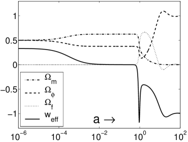
Figure 1: Background evolution when $\lambda=4$ and $\alpha=20$. In general, the evolution in the model consists of 1) the scaling attractor and 2) the potential-dominated (de Sitter) solution. Existence of 1) requires $\lambda>\sqrt{6}$, and the transition to 2) then occurs if $\alpha>\lambda$. Here we plot fractional energy densities for matter, $\Omega_{m}$ (dash-dotted line), scalar field $\Omega_{\phi}=(x^{2}+y)/3$ (dashed line) and the GB term, $\Omega_{f}=\mu$ (dotted line). Solid line is the total equation of state $w_{eff}=-2\epsilon/3-1$.

To investigate the cosmological effects of the GB coupling in more detail, we also consider the linear perturbations. In the synchronous gauge [21], one can parameterize the metric perturbations as

$$ds^{2}=-dt^{2}+a^{2}(t)(\delta_{ij}+h_{ij})dx^{i}dx^{j}.$$

Conventionally the scalar modes are then defined in the Fourier space by the decomposition into the trace ($h$) and the traceless part ($\eta$) of $h_{ij}$,

$$h_{ij}({\bf x},\tau)=\int d^{3}ke^{i{\bf k}\cdot{\bf x}}[\hat{k}_{i}\hat{k}_{j}h({\bf k},\tau)+6(\hat{k}_{i}\hat{k}_{j}-\frac{1}{3}\delta_{ij})\eta({\bf k},\tau)],$$

where ${\bf k}=k\hat{k}$. One can then write the energy constraint (perturbed version of the Friedmann equation) as an evolution equation for the metric potential $h$,

$$\dot{h}=\frac{8\pi G}{H(1-\frac{3}{2}\mu)}\left[2(1-\mu)\frac{\eta}{a^{2}}+\delta\rho+8H^{2}(3H\dot{\delta f}+\frac{k^{2}}{a^{2}}\delta f)\right].$$ (5)

where the density fluctuation is as usual $\delta\rho=\rho_{m}\delta_{m}+\dot{\phi}\dot{\delta\phi}+V^{\prime}(\phi)\delta\phi$. Note there appears both new source terms due to the fluctuations in the coupling $f$ as well as a modulating prefactor changing the response to the standard source terms. Similar modifications are present in the momentum constraint equation governing the evolution of the other metric potential $\eta$,

$$\dot{\eta}=\frac{4\pi G}{1-\mu}\left[a(\rho+p)\theta-8H(H\dot{\delta f}-H^{2}\delta f)\right],$$ (6)

where the velocity perturbation is as usual $a(\rho+p)\theta=a(\rho_{m}+p_{m})\theta_{m}+k\dot{\phi}\delta\phi$. The Klein-Gordon equation for the scalar field fluctuation, being the perturbed version of Eq.(4), is also non-trivially modified [22]. Since still minimally coupled to gravity, all other matter obey the usual continuity equations [20, 23].

We have numerically integrated the fully perturbed equations and computed the full matter power and CMBR spectra for the example model presented here.

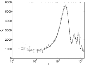
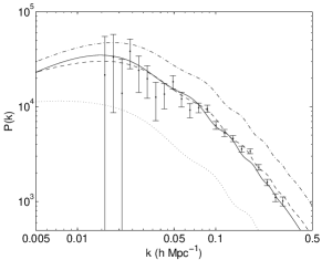
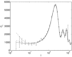
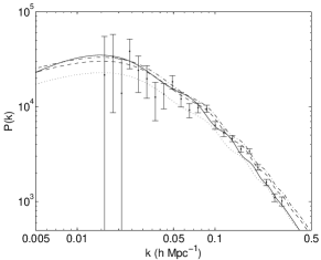
Figure 2: Top two figures: The effect of the potential slope on the CMB and matter power spectra. Here $\alpha=20$. Dotted lines are for $\lambda=4.5$, dashed line for $\lambda=6.0$, and dash-dotted for $\lambda=8.0$. Bottom two figures: The effect of the coupling slope on the CMB and matter power spectra. Here $\lambda=6.0$. Dotted lines are for $\alpha=10$, dashed line for $\alpha=20$, and dash-dotted for $\alpha=30$. The solid line is $\Lambda$CDM model. $\Omega_{m}^{0}=0.4$ for all figures. The CMB and matter power spectra error bars are from the WMAP data [3] and SDSS[2] respectively.

In FIG. 2 we show how the cosmological predictions are changed when the slope of the potential or of the coupling are varied. The main imprint from different potential slopes $\lambda$ seems to be in the normalization. For low values of $\lambda$, there is significant contribution of the scalar field during the matter dominated era. This slows down the rate of growth of matter inhomogeneities. Hence the fact that there is less structure nowadays than for larger $\lambda$ is not a consequence of the GB modification, but rather an effect of the presence of the scalar field in the earlier scaling era. Finally, in the bottom of FIG. 2 we see that the strength of the coupling $\alpha$ might be more difficult to deduce from these data. With steep coupling slopes, the scalar field domination takes place more rapidly and with more negative $w_{eff}$, which can somewhat amplify the ISW effect. The contrary happens for smaller $\alpha$.

We now consider the constraints arising from astrophysical and cosmological observations. We calculate the SNeIa luminosity-distance relation. To compare with data, we use the ”Gold” sample of 157 SNeIa from Ref. [1] and marginalize over the Hubble constant $H_{0}$. We also compute the CMBR shift parameter [24] $\mathcal{R}$ and apply the latest constraints [25]. The combined constraints arising from all these data is shown in FIG.3. The SNeIa data alone is consistent with a wide range of matter densities $\Omega_{m}$, but when combined with the CMBR parameter $\mathcal{R}$ one is restricted to rather high $\Omega_{m}\sim 0.4$. Note that we restrict here only to cosmologies where a scaling matter era is followed by the acceleration era. The existence of the scaling attractor requires $\lambda>\sqrt{6}$, otherwise the evolution is different and depends on the initial conditions for the field. Therefore we leave models with lower potential slopes, $\alpha<\sqrt{6}$, out from this study, but their phenomenology could be interesting to investigate elsewhere.

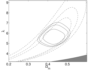
Figure 3: The 68, 90 and 99 percent confidence limits for the model in the $\Omega_{m}$ - $\lambda$ plane when $\alpha$ is marginalized over in the range $1.5\lambda<\alpha<10\lambda$. Dotted lines are constraints from the SNeIa data and the solid lines from the combined SNeIa and CMBR shift parameter data. In the gray area the scaling solution is unstable regardless of $\alpha$. If the scalar field is tracking already in the nucleosynthesis epoch, there is a tension with the amount of early quintessence and the nucleosynthesis limit. Conservatively, this limit would translate to $\lambda>6.3$ [4].

Time variation of the effective gravitational constant $G_{*}$ is tightly constrained by observations within the Solar system and laboratories, and indicate that $|G_{*}^{\prime}/G_{*}|\lesssim 0.01$ [26]. To derive the variation of this constant for the coupled GB gravity, we follow the approach of Ref. [27] where cosmological perturbation equations were considered at their Newtonian limit. The Poisson equation was derived and the effective strength of gravitational coupling was read from the resulting expression, which relates the gradient of the gravitational potential to the perturbations in matter density. The result in our case is

$$\frac{G_{*}}{G}=4\frac{-x^{4}+\mu^{2}(1+\epsilon)^{2}+x^{2}[2(1+\epsilon)(\mu-1)+y]}{x^{2}[4+\mu(5\mu-8)]-\mu^{2}[6(1+\epsilon)(\mu-1)+y]},$$ (7)

consistently with Ref. [27]. Though not obvious from the formula, it equals one when the coupling goes to zero. Generally, when $\mu$ is of order one, then one expects the $G_{*}^{\prime}/G_{*}$ to be of roughly of order one as well. As claimed in Ref. [27], one has to assume ”an accidental cancellation” to satisfy the bound for $G_{*}^{\prime}/G_{*}$ in the presence of significant GB contribution to the energy density. . This means that we have to fine-tune the coupling parameter $\alpha$ in order to eliminate the time variation of the effective gravitational coupling, typically with the accuracy of $0.01$. Then the Newtonian limit in general exhibits time-varying $G_{*}$, but at present days this $G_{*}$ appears to us as a constant. We have reported the cosmological results in such a case in Table 1. The best-fit values of $\chi^{2}$ per effective degree of freedom, $\chi^{2}_{dof}$, are slightly better than in the $\Lambda$CDM case.

Data set	$\Lambda$CDM		$R^{2}_{GB}\phi$ model
	$\chi^{2}_{dof}$	$\Omega_{m}$	$\chi^{2}_{dof}$	$\Omega_{m}$	$\lambda$	$\alpha$
SNeIa	$1.142$	$0.314$	1.146	0.42	5.1	32.3
SNeIa+$\mathcal{R}$	$1.144$	$0.277$	1.141	0.44	5.2	33.8

Table 1: Best-fit values for $\Lambda$CDM model compared with fits of the coupled scalar field model for some parameter values when the coupling $\alpha$ is set in order to fix the present time variation of $G_{*}$ to zero. The degrees of freedom in the first row are $157-d$, and in the second $158-d$, where $d=1$ for the $\Lambda$CDM and $d=3$ for the $R^{2}_{GB}\phi$ models.

Interestingly, $G_{*}$ determines the cosmological evolution of matter inhomogeneities at subhorizon scales. The matter overdensity $\delta$ evolves according to [20]

$$\ddot{\delta}+2H\dot{\delta}=4\pi G_{*}\rho\delta.$$ (8)

From this equation we can make the important conclusion that the evolution of matter inhomogeneities at small scales is independent of wavelenght. Thus we expect, given the same primordial spectrum of perturbations, the main difference in the matter power spectrum (when compared to $\Lambda$CDM) to be in the normalization. Note that to arrive at this result, we have not assumed specific forms for the coupling or the potential, but only that the scalar appearing in the action (2) is not very massive. Our numerical solutions of the whole perturbation system confirm that the approximation Eq.(8) indeed is good at subhorizon scales.

The effective gravitational constant $G_{*}$ can in principle diverge. We find that in the example model presented here, $G_{*}$ typically diverges in the future, and for low matter densities this can happen even before $a=1$. It is unclear what happens at such point, since the linear approximation certainly breaks down near the (what would be) singularity. Matter perturbations will at least for a while grow explosively. It is possible that consequently the de Sitter phase will not be then reached, which could help to define the S-matrix in string theory. This divergence can be related to previous stability considerations of these models (for recent studies, see Refs.[28, 30]). This far stability conditions for these models have been derived only in the case that the field perturbations decouple from other fluids. However, in dark energy cosmologies such as here one should take into account both matter and the corrections to Einstein gravity. We provide a clear indication that the scalar action in its vacuum form determines the stability also in the case that $\rho_{m}\neq 0$. The action for the potential $\Phi$ in vacuum features an effective propagation speed [22]

$$s_{SC}=\frac{-x^{2}[4+\mu(5\mu-8)]+\mu^{2}[6(1+\epsilon)(\mu-1)+y]}{(\mu-1)[3\mu^{2}-4(\mu-1)x^{2}]},$$ (9)

from which we can see that the linearized matter perturbations diverge exactly at the points where this propagation changes its sign .

To summarize, we studied a string-inspired low energy action where a coupling between a scalar field and the GB invariant is present. Solving the full system of equations which describe both the homogeneous universe as well as its first order perturbations we found several new insights to GB dark energy cosmologies in general, which could be relevant to future investigations of viable string-theory low energy effective actions. We showed that the background universe can present an attractor solution which features late transition from a scaling era to acceleration triggered by the GB coupling. This mechanism might be seen to alleviate the coincidence problem. In addition, the model can consistently explain a presently ongoing but transient phantom era. This background expansion can exhibit a good a accordance with cosmological and astrophysical data. The evolution of matter perturbations is scale-invariant at small scales in the presence of the GB term, and thus the shape of the matter power spectrum is retained. Hence, the latest data from the CMBR anisotropies as well as LSS can show agreement with these models. However, using a combined set of present days cosmological observations it is possible to constrain the parameters of the theory tightly.

References

- [1] A. G. Riess et al., Astrophys. J. 607, 665 (2004).
- [2] M. Tegmark et al., Phys. Rev. D69, 103501 (2004).
- [3] D. N. Spergel et al. (2006), astro-ph/0603449.
- [4] E. Copeland, M. Sami, and S. Tsujikawa hep-th/0603057.
- [5] S. Nojiri and S. D. Odintsov (2006), hep-th/0601213.
- [6] I. P. Neupane (2006a), hep-th/0605265.
- [7] S. Nojiri and S. D. Odintsov, Phys. Lett. B631, 1 (2005).
- [8] J. Callan et al., Nucl. Phys. B262, 593 (1985).
- [9] D. J. Gross and J. H. Sloan, Nucl. Phys. B291, 41 (1987).
- [10] I. Antoniadis, E. Gava, and K. S. Narain, Nucl. Phys. B383, 93 (1992), hep-th/9204030.
- [11] I. Antoniadis, J. Rizos, and K. Tamvakis, Nucl. Phys. B415, 497 (1994), hep-th/9305025.
- [12] S. Nojiri, S. D. Odintsov, and M. Sasaki, Phys. Rev. D71, 123509 (2005), hep-th/0504052.
- [13] B. Carter and I. P. Neupane , hep-th/0510109.
- [14] B. Carter and I. P. Neupane, hep-th/0512262.
- [15] I. P. Neupane (2006b), hep-th/0602097.
- [16] M. Sami et al., Phys. Lett. B619, 193 (2005).
- [17] G. Calcagni, S. Tsujikawa, and M. Sami, Class. Quant. Grav. 22, 3977 (2005), hep-th/0505193.
- [18] S. Nojiri, S. Odintsov, and M. Sami , hep-th/0605039.
- [19] M. Dine et al., Phys. Lett. B156, 55 (1985).
- [20] T. Koivisto and D. F. Mota, hep-th/0609155.
- [21] C. Ma and E. Bertschinger, Astrophys. J. 455, 7 (1995).
- [22] J.-c. Hwang and H. Noh, Phys. Rev. D71, 063536 (2005).
- [23] T. Koivisto Class. Quant. Grav. 23, 4289-4296 (2006).
- [24] C. J. Odman et al., D67, 083511 (2003).
- [25] Y. Wang and P. Mukherjee (2006), astro-ph/0604051.
- [26] J.-P. Uzan, Rev. Mod. Phys. 75, 403 (2003).
- [27] L. Amendola, C. Charmousis, and S. C. Davis (2005), hep-th/0506137.
- [28] A. De Felice, M. Hindmarsh, and M. Trodden (2006), astro-ph/0604154.
- [29] T. Clifton, D. F. Mota and J. D. Barrow, Mon. Not. Roy. Astron. Soc. 358, 601 (2005) [arXiv:gr-qc/0406001].
- [30] G. Calcagni, B. de Carlos, and A. De Felice (2006), hep-th/0604201.
- [31] A. Lewis, A. Challinor, and A. Lasenby, Astrophys. J. 538, 473 (2000), astro-ph/9911177.