Energy spectra of gamma-rays, electrons and neutrinos produced at proton-proton interactions in the very high energy regime

Abstract

We present new parametrisations of energy spectra of secondary particles, $\pi$-mesons, gamma-rays, electrons and neutrinos, produced in inelastic proton-proton collisions. The simple analytical approximations based on simulations of proton-proton interactions using the public available SIBYLL code, provide very good accuracy for energy distributions of secondary products in the energy range above 100 GeV. Generally, the recommended analytical formulae deviate from the simulated distributions within a few percent over a large range of $x=E_{i}/E_{p}$ - the fraction of energy of the incident proton transferred to the secondaries. Finally, we describe an approximate procedure of continuation of calculations towards low energies, down to the threshold of $\pi$-meson production.

I Introduction

Any reliable interpretation of an astronomical observation requires not only high quality experimental information concerning the spectral, temporal and spatial properties of radiation, but also unambiguous identification of the relevant radiation processes. In this regard, the good knowledge of characteristics of radiation mechanisms is a principal issue in astrophysics, in particular in gamma-ray astronomy where we often face a problem when the same observation can be equally well explained by two or more radiation processes.

Fortunately, all basic radiation processes relevant to high energy gamma-ray astronomy can be comprehensively studied using the methods and tools of experimental and theoretical physics. This concerns, in particular, one of the most principal gamma-ray production mechanisms in high-energy astrophysics – inelastic proton-proton interactions with subsequent decay of the secondary $\pi^{0}$ and $\eta$-mesons into gamma-rays. The decays of accompanying $\pi^{\pm}$-mesons and some other (less important) short-lived secondaries result in production of high energy neutrinos. This establishes a deep link between the high energy gamma-ray and neutrino astronomies. Finally, the secondary electrons (positrons) from p-p interactions may compete with directly accelerated electrons and thus significantly contribute to the nonthermal electromagnetic radiation of gamma-ray sources from radio to hard X-rays.

The principal role of this process in high energy astrophysics was recognized long ago by the pioneers of the field (see e.g. Morrison ; GinzSyr ; Hayakawa ), in particular in the context of their applications in gamma-ray (e.g. Stecker_book ) and neutrino (e.g. BerVol ) astronomies. The first reliable experimental results obtained with the SAS-2 and COS-B gamma-ray satellite missions, initiated new, more detailed studies of $\pi^{0}$-production in $p-p$ interactions StepBad1981 ; Dermer86 , in particular for the interpretation of the diffuse galactic gamma-ray background emission. The prospects of neutrino astronomy initiated similar calculations for high energy neutrinos and their links to gamma-ray astronomy Berez_Book ; Gaisser ; Berez91 ; Vissani .

The observations of diffuse gamma-ray emission from different parts of the galactic disk by EGRET revealed a noticeable excess of flux at energies of several GeV. Although this excess can be naturally explained by assuming somewhat harder proton spectrum (compared to the locally measured flux of cosmic rays) Mori ; AhAt00 ; StrongMosk00 , this result recently initiated a new study of the process Kamae05 based on the approach of separation of the diffractive and non-diffractive channels of interactions as well as incorporating violation of the Feynman scaling.

It is remarkable that while precise calculations of gamma-ray spectra require quite heavy integrations over differential cross-sections measured at laboratory experiments, the emissivity of gamma-rays for an arbitrary broad and smooth, e.g. power-law, energy distribution of protons can be obtained, with a quite reasonable accuracy, within a simple formalism (see e.g. Ref.AhAt00 ) based on the assumption of a constant fraction $\kappa$ of energy of the incident proton released in the secondary gamma-rays (see Torres for comparison of different approaches). This approach relies on the energy-dependent total inelastic cross-section of pp interactions, $\sigma_{\rm pp}^{\rm inel}(E)$, and assumes a fixed value of the parameter $\kappa\approx 0.17$, which provides the best agreement with the accurate numerical calculations over a wide energy range of gamma-rays.

On the other hand, in the case of sharp spectral features like pileups or cutoffs in the proton energy distribution, one has to perform accurate numerical calculations based on simulations of inclusive cross-sections of production of secondary particles. Presently three well developed codes of simulations of p-p interactions are public available – Pythia Pythia_model , SIBYLL SIBYLL_model , QGSJET QGSJET_model . The last two as well as some other models are combined in the more general CORSIKA code CORSIKA designed for simulations of interactions of cosmic rays with the Earth atmosphere. These codes are based on phenomenological models of p-p interactions incorporated with comprehensive experimental data obtained at particle accelerators.

While these codes can be directly used for calculations of gamma-ray spectra for any distribution of primary protons, it is quite useful to have simple analytical parameterizations which not only significantly reduce the calculation time, but also allow better understanding of characteristics of secondary electrons, especially for the distributions of parent protons with distinct spectral features. This concerns, for example, such an important question as the extraction of the shape of the proton energy distribution in the cutoff region based on the analysis of the observed gamma-ray spectrum. Indeed, while the delta-functional approach implies, by definition, similar spectral shapes of gamma-rays and protons (shifted in the energy scale by a factor of $\kappa$), in reality the energy spectrum of highest energy gamma-rays appears, as we show below, smoother than the distribution of protons in the corresponding (cutoff) region. Thus, the use of simple approximations not always can be justified, and, in fact, they may cause misleading astrophysical conclusions about the energy spectra of accelerated protons.

Two different parameterizations of inclusive cross-sections for pion-production in proton-proton interactions has been published by Stephens and Badwar StepBad1981 and Blattnig et al Blattnig . However, recently it was recognized Torres that both parameterizations do not describe correctly the gamma-ray spectra in the high energy regime. The parameterization of Stephens and Badwar underpredicts the yield of high energy pions. The parameterization by Blattnig et al. is valid for energies below 50 GeV; above this energy it significantly overpredicts the pions production.

In this paper we present new parameterizations for high energy spectra of gamma-rays, electrons and neutrinos based on the simulations of proton-proton interactions using the SIBYLL code SIBYLL_model , and partly (only for distributions of $\pi$-mesons) the QGSJET QGSJET_model code. We provide simple analytical approximations for the energy spectra of secondaries with accuracies generally better than several percent.

II Inclusive spectra of pions

The energy spectra of secondary products of p-p interactions $F_{\pi}(x,\,E_{p})$ are expressed through the total and inclusive cross-sections,

$$F_{\pi}(x,\,E_{p})=\frac{E_{p}}{\sigma_{\rm inel}}\int\frac{d^{3}\sigma}{dp^{3}}\ d^{2}p_{t}\ ,$$ (1)

where $x=E_{\pi}/E_{p}$ is the ratio of the energy of incident proton $E_{p}$ transferred to the secondary $\pi$-meson. It is convenient to present $F_{\pi}(x,\,E_{p})$ in the form

$$F_{\pi}(x,\,E_{p})=\frac{d}{dx}\,\Phi(x,\,E_{p})\,.$$ (2)

By definition

$$dN_{\pi}\equiv F_{\pi}(x,\,E_{p})\,dx=F_{\pi}(x,\,E_{p})\,dE_{\pi}/E_{p}$$ (3)

is the number of neutral $\pi$-mesons per one $p-p$ interaction in the energy interval $(E_{\pi}\,,\,E_{\pi}+dE_{\pi})$. The presentation in the form of Eq.(2) is convenient because it allows to estimate easily the multiplicity of $\pi$-mesons. The function $\Phi(x,\,E_{p})$ obviously can be presented in different forms. For the simulated distributions obtained with the QGSJET model (see Fig. 1) the function

$$\Phi_{\rm QGSJET}=-B_{\pi}\left(\frac{1-x^{\alpha}}{(1+r\,x^{\alpha})^{3}}\right)^{4}\,,$$ (4)

provides a rather good fit with the parameters $B_{\pi}$, $\alpha$ and $r$ as weak functions of $E_{p}$. Note that

$$\int\limits_{0}^{1}\!F_{\pi}(x,\,E_{p})\,dx=B_{\pi}\,.$$ (5)

Also, at the threshold, $x=m_{\pi}/E_{p}$, the function $F_{\pi}$ should approach zero. In order to take this effect into account, we introduce an additional term $(1-m_{\pi}/(x\,E_{p}))^{1/2}$ and require that $F_{\pi}=0$ at $x<m_{\pi}/E_{p}$. Then we obtain

$$F_{\pi}(x,\,E_{p})=4\,\alpha B_{\pi}x^{\alpha-1}\left(\frac{1-x^{\alpha}}{(1+r\,x^{\alpha})^{3}}\right)^{4}\times$$

$$\left(\frac{1}{1-x^{\alpha}}+\frac{3\,r}{1+rx^{\alpha}}\right)\left(1-\frac{m_{\pi}}{x\,E_{p}}\right)^{1/2}.$$ (6)

The spectra of charged pions are described by the same equation.

The parameters $B_{\pi}$, $\alpha$, and $k$ were obtained via the best least squares fits to the simulated events (histogram in Fig. 1). For the energy interval of incident protons $0.1-10^{3}$ TeV this procedure gives

$$B_{\pi}=5.58+0.78\,L+0.10\,L^{2}\,,$$ (7)

$$r=\frac{3.1}{B_{\pi}^{3/2}}\,,\quad\alpha=\frac{0.89}{B_{\pi}^{1/2}\left(1-e^{-0.33\,B_{\pi}}\right)}\,,$$ (8)

where $L=\ln(E_{p}/1\,{\rm TeV})$.

For $x\gtrsim 10^{-3}$ (provided that $E_{\pi}\geq 10\ \rm GeV$) this analytical approximation deviates from simulations less than 10 percent for the entire energy range of incident protons from 0.1 to $10^{3}$ TeV. In Fig. 1 the results of the QGSJET simulations and the fits based on Eq.(6) are shown for the proton energies of 0.1 TeV and $10^{3}$ TeV.

 

Figure 1: Energy spectra of neutral pions from the numerical simulations of the QGSJET code (histograms) and from the presentation given by Eq.(6) for two energies of primary protons: (a) 0.1 TeV and (b) $10^{3}$ TeV.

The results of numerical simulations of the energy distribution of secondary pions obtained with the SIBYLL code are well described by the function

$$\Phi_{\rm SIBYLL}=-B_{\pi}\left(\frac{1-x^{\alpha}}{1+r\,x^{\alpha}\,(1-x^{\alpha})}\right)^{4}\,,$$ (9)

with the best fit parameters

$$B_{\pi}=a+0.25\,,\quad\alpha=\frac{0.98}{\sqrt{a}}\,,\,r=\frac{2.6}{\sqrt{a}}\,,$$ (10)

where

$$a=3.67+0.83\,L+0.075\,L^{2}\,,\quad L=\ln(E_{p}/1\,{\rm TeV})\,.$$ (11)

From Eqs.(9) and (2), and introducing an additional term $(1-m_{\pi}/(x\,E_{p}))^{1/2}$, one obtains

$$F_{\pi}(x,\,E_{p})=4\alpha B_{\pi}x^{\alpha-1}\left(\frac{1-x^{\alpha}}{1+rx^{\alpha}(1-x^{\alpha})}\right)^{4}\times$$

$$\left(\frac{1}{1-x^{\alpha}}+\frac{r\,(1-2x^{\alpha})}{1+rx^{\alpha}(1-x^{\alpha})}\right)\left(1-\frac{m_{\pi}}{x\,E_{p}}\right)^{1/2}\,.$$ (12)

In the context of different astrophysical applications, the ultimate aim of this study is the analytical description of gamma-rays and lepton from decays of unstable secondary particles produced at proton-proton interactions. In this regard, in the case of gamma-rays one has to consider, in addition to $\pi^{0}$-mesons, also production and decay of $\eta$-mesons. The analysis of the simulations show that the energy spectrum of $\eta$-mesons is well described by the function

$$F_{\eta}(x,\,E_{p})=(0.55+0.028\,\ln x)\left(1-\frac{m_{\eta}}{x\,E_{p}}\right)F_{\pi}(x,\,E_{p})$$ (13)

with the condition $F_{\eta}(x,\,E_{p})=0$ at $x<m_{\eta}/E_{p}$.

In Fig. 2 we present the results of simulations of energy distributions of $\pi$- and $\eta$-mesons obtained with the SIBYLL code, together with the analytical approximations given by Eqs. (12) and (13) for four energies of incident protons: 0.1, 10, 100, and 1000 TeV. Note that Eq.(12) describes the spectra of pions at $x\gtrsim 10^{-3}$ with an accuracy better than 10 percent over the energy range of protons from 0.1 TeV to $10^{5}\;{\rm TeV}$. The approximation for the spectrum of $\eta$-mesons is somewhat less accurate. However, since the contribution of $\pi^{0}$-mesons to gamma-rays dominates over the contribution from decays of $\eta$-mesons, accuracy of Eq. (13) is quite acceptable.

   

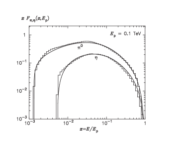
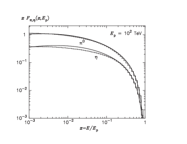
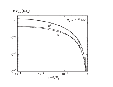
Figure 2: Energy spectra of $\pi$- and $\eta$-mesons from the numerical simulations of the SIBYLL code (histograms) and from the analytical presentations given by Eqs. (12) and (13) for four energies of primary protons: (a) 0.1 TeV, (b) 10 TeV, (c) 100 TeV, (d) 1000 TeV.

The QGSJET and SIBYLL codes give quite similar, but not identical results. The differences are reflected in the corresponding analytical presentations. In Fig.3 the energy spectra of pions described by Eqs.(4) and (12) are shown for two energies of protons. While these two approximations give similar results around $x\sim 0.1$, deviations at very small, $x\leq 10^{-2}$, and very large, $x\geq 0.5$, energies of secondary pions, are quite significant. Generally, the gamma-ray spectra from astrophysical objects are formed at a single p-p collision (the so-called "thin target" scenario), therefore the most important contribution comes from the region $x=E_{\pi}/E_{0}\sim 0.1$, where these two approximations agree quite well with each other. On the other hand, for the proton distributions with distinct spectral features, in particular with sharp high-energy cutoffs, the region of $x\geq 0.1$ plays important role in the formation of the corresponding high-energy spectral tails of secondary products. Since it appears that in this range the SIBYLL code describes the accelerator data somewhat better (Sergey Ostapchenko, private communication), in the following sections we will use the distributions of secondary hadrons obtained with the SIBYLL code to parameterize the energy spectra of the final products of p-p interactions - gamma-rays, electrons and neutrinos.

Figure 3: Comparison of the energy distributions of secondary $\pi$-mesons given by Eq.(4) (dashed curves) and Eq.(12) (solid curves) calculated for two energies of parent protons $E_{p}=1$ TeV and 100 TeV.

III Decay of pions

In this section we discuss the energy spectra of decay products of neutral and charged ultrarelativistic $\pi$-mesons.

III.1 $\pi^{0}\to\gamma\gamma$

The energy distribution of gamma-rays from the decay of $\pi^{0}$-mesons with spectrum $J_{\pi}(E_{\pi})$ reads

$$Q_{\gamma}(E_{\gamma})=2\int\limits_{E_{\gamma}}^{\infty}\!J_{\pi}(E_{\pi})\,\frac{dE_{\pi}}{E_{\pi}}\,,$$ (14)

with total number of photons

$${\cal N}_{\gamma}=\int\limits_{0}^{\infty}\!Q_{\gamma}(E_{\gamma})\,dE_{\gamma}=2\int\limits_{0}^{\infty}\!dE_{\gamma}\int\limits_{E_{\gamma}}^{\infty}\frac{dE_{\pi}}{E_{\pi}}\,J_{\pi}(E_{\pi})\,.$$ (15)

By changing the order of integration, and integrating over $dE_{\gamma}$, one obtains an obvious relation

$${\cal N}_{\gamma}=2\int\limits_{0}^{\infty}\!J_{\pi}(E_{\pi})\,dE_{\pi}=2\,{\cal N}_{\pi}\,.$$ (16)

The total energy of gamma-rays also coincides with the total energy of pions:

$${\cal E}_{\gamma}=\int\limits_{0}^{\infty}\!E_{\gamma}\,Q_{\gamma}(E_{\gamma})\,dE_{\gamma}=\int\limits_{0}^{\infty}\!E_{\pi}\,J_{\pi}(E_{\pi})\,dE_{\pi}={\cal E}_{\pi}\,.$$ (17)

Let’s consider a simple example assuming that the spectrum of pions has a power-law form with a low energy cutoff at $E_{0}$:

$$J_{\pi}(E_{\pi})=\left\{\begin{array}[]{cl}A/(E_{\pi})^{\alpha}\,,&\quad E_{\pi}>E_{0}\,,\\ 0\,,&\quad E_{\pi}<E_{0}\,,\end{array}\right.$$ (18)

where $A$, $E_{0}$ and $\alpha$ are arbitrary constants. For $\alpha>2$ the number of pions and their total energy are equal

$${\cal N}_{\pi}=\frac{A}{(\alpha-1)E_{0}^{\alpha-1}}\,,\quad{\cal E}_{\pi}=\frac{A}{(\alpha-2)E_{0}^{\alpha-2}}\,,$$ (19)

while the energy spectrum of gamma-rays has the following form

$$Q_{\gamma}(E_{\gamma})=\left\{\begin{array}[]{cl}\displaystyle\frac{2\,A}{\alpha E_{\gamma}^{\alpha}}\,,&\quad E_{\gamma}>E_{0}\,,\\[12.0pt] \displaystyle\frac{2\,A}{\alpha E_{0}^{\alpha}}\,,&\quad E_{\gamma}<E_{0}\,.\end{array}\right.$$ (20)

Above the energy $E_{0}$, the gamma-ray spectrum repeats the shape of the pion spectrum; below $E_{0}$ the gamma-ray spectrum is energy-independent.

Note that in the region $E>E_{0}$ the number of gamma-rays of given energy $E$ is less than the number of pions of same energy. Indeed,

$$R_{\gamma}\equiv\frac{Q_{\gamma}(E)}{J_{\pi}(E)}=\frac{2}{\alpha}<1\,,\quad\mbox{at}\;\;E>E_{0}\,.$$ (21)

On the other hand, since the total number of gamma-rays by a factor of 2 exceeds the total number of pions, one should expect more gamma-rays at low energies. Indeed, the numbers of gamma-rays above and below $E_{0}$ are

$${\cal N}_{\gamma}(E_{\gamma}>E_{0}) = \frac{2\,A}{\alpha(\alpha-1)E_{0}^{\alpha-1}}\,,$$

$${\cal N}_{\gamma}(E_{\gamma}<E_{0}) = \frac{2\,A}{\alpha E_{0}^{\alpha-1}}\,.$$

Although ${\cal N}_{\gamma}(E_{\gamma}>E_{0})/{\cal N}_{\pi}=R_{\gamma}<1$, the sum

$${\cal N}_{\gamma}(E_{\gamma}>E_{0})+{\cal N}_{\gamma}(E_{\gamma}<E_{0})=2\,{\cal N}_{\pi}\,.$$ (22)

One may say that the "deficit" of the number of high energy gamma-rays is compensated by the "excess" of low energy gamma-rays.

III.2 $\pi\to\mu\nu_{\mu}$

In the rest frame of the pion, the energy of secondary muons and neutrinos from the $\pi\to\mu\nu_{\mu}$ decays are

$$E_{\mu}^{0}=\frac{m_{\pi}^{2}+m_{\mu}^{2}}{2\,m_{\pi}}\,,\quad E_{\nu}^{0}=\frac{m_{\pi}^{2}-m_{\mu}^{2}}{2\,m_{\pi}}\,.$$ (23)

The momenta of secondaries in this system are

$$p_{\mu}^{0}=p_{\nu}^{0}=E_{\nu}^{0}\,.$$ (24)

In the laboratory frame of coordinates (L-frame) and for $E_{\pi}\gg m_{\pi}$

$$E_{\nu,\max}=\frac{1}{m_{\pi}}\,(E_{\pi}E_{\nu}^{0}+p_{\pi}p_{\nu}^{0})\approx\lambda\,E_{\pi}\,,$$ (25)

where

$$\lambda=1-m_{\mu}^{2}/m_{\pi}^{2}=0.427\ .$$ (26)

Thus, the muonic neutrinos produced at the decay of an ultrarelativistic pion of energy $E_{\pi}$ are distributed as $dE_{\nu}/\lambda\,E_{\pi}$ ($0<E_{\nu}<\lambda\,E_{\pi}$). Correspondingly, if the energy distribution of pions is described by function $J_{\pi}(E_{\pi})$, for neutrinos produced at the decay $\pi\to\mu\nu_{\mu}$

$$Q_{\nu}(E_{\nu})=\int\limits_{E_{\nu}/\lambda}^{\infty}\!J_{\pi}(E_{\pi})\,\frac{dE_{\pi}}{\lambda\,E_{\pi}}\,.$$ (27)

For example, in the case of pion distribution given by Eq.(18), one has

$$Q_{\nu}(E_{\nu})=\left\{\begin{array}[]{cl}\displaystyle\frac{\lambda^{\alpha-1}A}{\alpha E_{\nu}^{\alpha}}\,,&\quad E_{\nu}>\lambda E_{0}\,,\\[12.0pt] \displaystyle\frac{A}{\alpha\lambda E_{0}^{\alpha}}\,,&\quad E_{\nu}<\lambda E_{0}\,.\end{array}\right.$$ (28)

The ratio of neutrinos to pions of same energy is

$$R_{\nu}=\frac{Q_{\nu}(E)}{J_{\pi}(E)}=\frac{\lambda^{\alpha-1}}{\alpha}<1\,,\quad\mbox{at}\;\;E>E_{0}\,.$$ (29)

Note that the factor $\lambda^{\alpha-1}$ significantly reduces the number of neutrinos relative to their counterpart gamma-rays from decays of neutral pions.

III.3 $\mu\to e\nu_{e}\nu_{\mu}$

The treatment of this three-particle-decay channel is more complex. Since $m_{\mu}\gg m_{e}$, in calculations we will neglect the mass of electrons. Then the maximum energy of the muon in the L-frame is

$$E_{\mu,\max}=\frac{1}{m_{\pi}}\,(E_{\pi}E_{\mu}^{0}+p_{\pi}p_{\mu}^{0})\approx E_{\pi}\,.$$ (30)

Thus, the spectra of all particles produced at the decay of muons will continue up to the energy $E_{\pi}$ (note that the neutrinos from the decay of charge pions continue to $0.427E_{\pi}$). The formalism of calculations of energy distributions of secondary products from decays of muons is described in Gaisser ; Lipari .

In $\pi\to\mu+\nu_{\mu}$ decays muons are fully polarized. In this case the energy and angular distribution of electrons (and muonic neutrinos) in the rest frame of muon is described by the function (see e.g. Okun )

$$g_{e}(E^{\prime}_{e},\tilde{\theta}^{\prime})=\frac{1}{\pi m_{\mu}}\,\tau^{2}\left[3-2\tau\mp(1-2\tau)\cos\tilde{\theta}^{\prime}\right]\,,$$ (31)

where $\tau={2E^{\prime}_{e}}/{m_{\mu}}$, $\tilde{\theta}^{\prime}$ is the angle between the momentum of electron (neutrino) and the spin of muon. The signs $\mp$ of the second term in Eq.(31) correspond to the decays of $\mu^{+}$ and $\mu^{-}$, respectively.

While the distribution of muonic neutrinos is identical to the distribution of electrons, the distribution $g_{\nu_{e}}(E^{\prime}_{\nu_{e}},\theta^{\prime})$ of electronic neutrinos has the following form:

$$g_{\nu_{e}}(E^{\prime}_{\nu_{e}},\tilde{\theta}^{\prime})=\frac{6}{\pi m_{\mu}}\,\tau^{2}(1-\tau)\left(1\mp\cos\tilde{\theta}^{\prime}\right)\,,$$ (32)

where $\tau={2E^{\prime}_{\nu_{e}}}/{m_{\mu}}$ In the rest frame of the muon the maximum energy of each particle is $m_{\mu}/2$. The functions given by Eqs.(31) and (32) are normalized as

$$\int\!g(E^{\prime},\tilde{\theta}^{\prime})\,dE^{\prime}\,d\Omega^{\prime}=1\,.$$ (33)

Let’s denote the angle between the muon momentum in the rest frame of the pion and the electron momentum in the rest frame of muon as $\theta^{\prime}$. Since the spin of $\mu^{-}$ is parallel to the momentum, $\theta^{\prime}=\tilde{\theta}^{\prime}$, while for $\mu^{+}$ we have $\theta^{\prime}=\pi-\tilde{\theta}^{\prime}$ (the spin is anti-parallel to the momentum). Therefore the energy and angular distributions of electrons (expressed through $\theta^{\prime}$), from $\mu^{+}$ and $\mu^{-}$ decays have the same form:

$$g_{e}(E^{\prime}_{e},\theta^{\prime})=\frac{1}{\pi m_{\mu}}\,\tau^{2}\left[3+2\tau\,(1-2\tau)\cos\theta^{\prime}\right]\,,$$ (34)

For the electronic neutrino we have

$$g_{\nu_{e}}(E^{\prime}_{\nu_{e}},\theta^{\prime})=\frac{6}{\pi m_{\mu}}\,\tau^{2}(1-\tau)\left(1+\cos\theta^{\prime}\right)\,.$$ (35)

It is easy to obtain, after Lorentz transformations, the angular and energy distributions of the decay products, $g_{i}(E,\theta)$, in the L-frame. The integration of $g_{i}(E,\theta)$ over the solid angle gives the corresponding energy distributions of particles $f_{i}(E)$. These functions are derived in the Appendix. Note that the energy distribution of leptons from the $\pi^{+}$ and $\pi^{-}$-meson decays are identical because of the CP invariance of weak interactions. In this regard we should note that the statement of Ref.Mosk about the "$e^{\pm}$ asymmetry" is not correct.

For ultrarelativistic $\pi$-mesons the result can be presented in the form of functions of variable $x=E/E_{\pi}$, where $E$ is the energy of the lepton. Let’s denote the probability of appearance of the variable $x$ within the interval $(x,x+dx)$ as $dw=f(x)\,dx$. The analytical integration gives the following distributions for electrons and muonic neutrinos:

$$f_{e}(x)=f_{\nu_{\mu}^{(2)}}(x)=g_{\nu_{\mu}}(x)\,\Theta(x-r)+$$

$$(h^{(1)}_{\nu_{\mu}}(x)+h^{(2)}_{\nu_{\mu}}(x))\,\Theta(r-x)\,,$$ (36)

where $r=1-\lambda=(m_{\mu}/m_{\pi})^{2}=0.573$,

$$g_{\nu_{\mu}}(x)=\frac{3-2r}{9(1-r)^{2}}\,\left(9x^{2}-6\ln x-4x^{3}-5\right),$$ (37)

$$h^{(1)}_{\nu_{\mu}}(x)=\frac{3-2r}{9(1-r)^{2}}\,\left(9r^{2}-6\ln r-4r^{3}-5\right),$$ (38)

$$h^{(2)}_{\nu_{\mu}}(x)=\displaystyle\frac{(1+2r)(r-x)}{9r^{2}}\times$$

$$\left[9(r+x)-4(r^{2}+rx+x^{2})\right]\ ,$$ (39)

$\Theta$ is the Heaviside function ($\Theta(x)=1$ if $x\geq 0$, and $\Theta(x)=0$ for $x<0$).

For electronic neutrinos

$$f_{\nu_{e}}(x)=g_{\nu_{e}}(x)\,\Theta(x-r)+$$

$$(h^{(1)}_{\nu_{e}}(x)+h^{(2)}_{\nu_{e}}(x))\,\Theta(r-x)\,,$$ (40)

where

$$g_{\nu_{e}}(x)=\displaystyle\frac{2(1-x)}{3(1-r)^{2}}\times$$

$$\left[6(1-x)^{2}+r(5+5x-4x^{2}))+6r\ln x\right]\,,$$ (41)

$$h^{(1)}_{\nu_{e}}(x)=\displaystyle\frac{2}{3(1-r)^{2}}\times$$

$$\left[(1-r)(6-7r+11r^{2}-4r^{3})+6r\ln r\right],$$ (42)

$$h^{(2)}_{\nu_{e}}(x)=\displaystyle\frac{2(r-x)}{3r^{2}}\times$$

$$\left(7r^{2}-4r^{3}+7xr-4xr^{2}-2x^{2}-4x^{2}r\right).$$ (43)

The functions are normalized

$$\int\limits_{0}^{1}\!f_{\nu_{\mu}^{(2)}}(x)\,dx=\int\limits_{0}^{1}\!f_{\nu_{e}}(x)\,dx=1\,.$$ (44)

At $x=0$ one has $f_{\nu_{\mu}^{(2)}}(0)=2.214$ and $f_{\nu_{e}}(0)=2.367$, while at $x\to 1$ the functions behave as

$$f_{\nu_{\mu}^{(2)}}(x)=\frac{2(3-2r)(1-x)^{3}}{3(1-r)^{2}}\,,\quad f_{\nu_{e}}(x)=\frac{4(1-x)^{3}}{1-r}\,.$$ (45)

It is possible to obtain simple analytical presentations also for the so-called Z-factors:

$$Z_{\nu_{\mu}}^{(2)}(\alpha)\equiv\int\limits_{0}^{1}\!x^{\alpha-1}f_{\nu_{\mu}^{(2)}}(x)\,dx=$$

$$\displaystyle\frac{4[3-2r-r^{\alpha}(3-2r+\alpha-\alpha r)]}{\alpha^{2}(1-r)^{2}(\alpha+2)(\alpha+3)}\,,$$ (46)

$$Z_{\nu_{e}}(\alpha)\equiv\int\limits_{0}^{1}\!x^{\alpha-1}f_{\nu_{e}}(x)\,dx=$$

$$\displaystyle\frac{24[\alpha(1-r)-r(1-r^{\alpha})]}{\alpha^{2}(1-r)^{2}(\alpha+1)(\alpha+2)(\alpha+3)}\,.$$ (47)

For comparison, for $\gamma$-rays and neutrinos from the $\pi\to\mu\nu_{\mu}$ decay, one has

$$Z_{\gamma}=2/\alpha\ ,$$ (48)

and

$$Z_{\nu_{\mu}}^{(1)}=\lambda^{\alpha-1}/\alpha\,,$$ (49)

where $\lambda$ is defined by Eq.(26).

In Fig. 4 we show the functions $dw/dx$ for different decay products in the L-frame. Note that the distributions of electrons and muonic neutrinos produced at decays of muons simply coincides. In the same figure we show also the distributions of photons (from the decay $\pi^{0}\to 2\gamma$ of neutral pions) and muonic neutrinos (from the decays $\pi\to\mu\nu_{\mu}$ of charged pions). The curves corresponding to the distribution of muonic neutrinos are marked by symbols $\nu_{\mu}^{(1)}$ for the neutrinos from the direct decay $\pi\to\mu\nu_{\mu}$ and $\nu_{\mu}^{(2)}$ for the neutrinos from the decay $\mu\to e\nu_{\mu}\nu_{e}$. All functions are normalized, $\int_{0}^{1}\!dw=1$.

Figure 4: Energy distributions of the secondary products (photons, electrons, muonic and electronic neutrinos) of decays of monoenergetic ultrarelativistic neutral and charged pions. All distributions are normalized, $\int_{0}^{1}\!dw=1$.

III.4 Energy spectra of decay products for arbitrary energy distributions of pions

The spectra of secondary products of decays of pions of arbitrary energy distributions $J_{\pi}(E_{\pi})$ (the number of pions in the energy interval $(E_{\pi},\,E_{\pi}+dE_{\pi})$ is equal $dN_{\pi}(E_{\pi})=J_{\pi}(E_{\pi})\,dE_{\pi}$) are determined by integration over the pion energy. In particular, for gamma-rays

$$Q_{\gamma}(E_{\gamma})=2\int\limits_{0}^{1}\!J_{\pi}\!\left(\frac{E_{\gamma}}{x}\right)\frac{dx}{x}\,.$$ (50)

The factor 2 implies that at the decay of $\pi^{0}$-meson two photons are produced. Similarly for the electrons and electronic neutrinos

$$Q_{e}(E_{e})=2\int\limits_{0}^{1}\!f_{e}(x)\,J_{\pi}\!\left(\frac{E_{e}}{x}\right)\frac{dx}{x}\,,$$ (51)

$$Q_{\nu_{e}}(E_{\nu_{e}})=2\int\limits_{0}^{1}\!f_{\nu_{e}}(x)\,J_{\pi}\!\left(\frac{E_{\nu_{e}}}{x}\right)\frac{dx}{x}\,.$$ (52)

Here the factor 2 takes into account the contributions from both $\pi^{+}$ and $\pi^{-}$ pions.

Finally, for muonic neutrinos we have

$$Q_{\nu_{\mu}}(E_{\nu_{\mu}})=2\int\limits_{0}^{1}\!(f_{\nu_{\mu}^{(1)}}(x)+f_{\nu_{\mu}^{(2)}}(x))\,J_{\pi}\!\left(\frac{E_{\nu_{\mu}}}{x}\right)\frac{dx}{x}=$$

$$\frac{2}{\lambda}\int\limits_{0}^{\lambda}\!J_{\pi}\!\left(\frac{E_{\nu_{e}}}{x}\right)\frac{dx}{x}+2\int\limits_{0}^{1}\!f_{\nu_{\mu}^{(2)}}(x)\,J_{\pi}\!\left(\frac{E_{\nu_{\mu}}}{x}\right)\frac{dx}{x}\,.$$ (53)

The first and second terms of Eq.(53) describe the muonic neutrinos produced through the direct decay $\pi\to\mu\nu_{\mu}$ of the pion and the decay of the secondary muon, respectively. Note that in Eqs.(51) – (53) we do not distinguish between electrons and positrons , as well as between neutrinos and antineutrinos. In fact, in $p-p$ interactions the number of $\pi^{+}$- mesons slightly exceeds the number of $\pi^{-}$ even at energies far from the threshold. However, this effect is less than the accuracy of both the measurements and our analytical approximations, therefore we will adopt $\nu=\bar{\nu}$ and $e^{+}=e^{-}$.

Figure 5: The ratio of the number of leptons to photons of same energy for power-law distributions of pions with spectral index $\alpha$. It is assumed that $\pi^{0}$, $\pi^{+}$ and $\pi^{-}$ have identical distributions.

It is of practical interest to compare the spectra of the secondary particles for power-law distributions of pions. Namely, let assume that the energy distributions of $\pi^{0}$, $\pi^{-}$ and $\pi^{+}$ mesons are distributed by Eq.(18) with an arbitrary spectral index $\alpha$. Then in the energy region $E>E_{0}$ the energy spectra of photons and leptons are power-law with the same spectral index $\alpha$. The ratio of leptons to photons of same energy depends only on $\alpha$. For the muonic neutrinos, electrons, and electronic neutrinos these ratios are

$$\frac{N_{\nu_{\mu}}}{N_{\gamma}}=\lambda^{\alpha-1}+\alpha\int\limits_{0}^{1}\!f_{e}(x)\,x^{\alpha-1}\,dx\,,$$ (54)

$$\frac{N_{e}}{N_{\gamma}}=\alpha\int\limits_{0}^{1}\!f_{e}(x)\,x^{\alpha-1}\,dx\,,$$ (55)

$$\frac{N_{\nu_{e}}}{N_{\gamma}}=\alpha\int\limits_{0}^{1}\!f_{\nu_{e}}(x)\,x^{\alpha-1}\,dx\,.$$ (56)

The ratios given by Eqs.(54), (55) and (56) as functions of $\alpha$ are shown in Fig. 5. Note that only in the case of $\alpha=1$ the ratio $N_{\rm leptons}/N_{\gamma}$ coincides with the ratio of the total number of leptons to gamma-rays. With increase of $\alpha$ the lepton/photon ratio decreases. For example, for $\alpha=2$ one has $N_{\nu_{\mu}}/N_{\gamma}=0.96$, $N_{e}/N_{\gamma}=0.53$, $N_{\nu_{e}}/N_{\gamma}=0.52$. For $\alpha=2.5$ these ratios are 0.68, 0.40, 0.39, respectively. Finally, note that the spectra of electrons and electronic neutrinos are very similar, thus the corresponding curves in Fig.5 practically coincide.

IV Energy spectra of photons and leptons produced at p-p collisions

For calculations of the energy spectra of gamma-rays, neutrinos and electrons produced at p-p interactions one should substitute the distribution of pions $F_{\pi}(x,\,E_{p})$ given by Eq. (12) into Eqs.(50) – (53):

$$J_{\pi}(E_{\pi})\,dE_{\pi}\to F_{\pi}(x,\,E_{p})\,dx=F_{\pi}\!\left(\frac{E_{\pi}}{E_{p}},\,E_{p}\right)\,\frac{dE_{\pi}}{E_{p}}\,.$$ (57)

The incident proton energy $E_{p}$ enters this equation as a free parameter.

IV.1 Spectra of gamma-rays

For calculations of gamma-ray spectra one should include the contribution also from $\eta$-mesons. The main modes of decay of $\eta$-mesons are ParticleData : $\eta\to 2\,\gamma$ (39.4%); $\eta\to 3\,\pi^{0}$ (32.5%); $\eta\to\pi^{+}\pi^{-}\pi^{0}$ (22.6%) and $\eta\to\pi^{+}\pi^{-}\gamma$ (5%). Approximately 3.2 gamma-ray photons are produced per decay of $\eta$-meson; the energy transferred to all gamma-rays is $0.81\,E_{\eta}$.

The spectrum of gamma-rays produced in the direct $\eta\to 2\,\gamma$ decay is calculated similarly to the decay of $\pi^{0}$-mesons. For accurate calculation of gamma-ray spectra from the decay chains $\eta\to 3\,\pi^{0}\to 6\gamma$ and $\eta\to\pi^{+}\pi^{-}\pi^{0}\to 2\gamma$, one has to know, strictly speaking, the function of energy distribution of pions $g(E_{\pi}^{0})$ in the rest frame of the $\eta$-meson, and then calculate, through Lorentz transformations, the distribution of pions in the L-frame. However, the calculations with model functions show that the spectrum of gamma-rays weakly depends on the specific form of $g(E_{\pi}^{0})$; for different extreme forms of function $g(E_{\pi}^{0})$ the results vary within 5 percent.

The maximum energy of pions in the rest frame of $\eta$-meson is $E^{0}_{\pi\max}=(m_{\eta}^{2}-3\,m_{\pi}^{2})/(2\,m_{\eta})$, while in the L-frame $E_{\pi\max}=\left(E^{0}_{\pi\max}+p^{0}_{\pi\,\max}\right)E_{\eta}/m_{\eta}\approx 0.73\,E_{\eta}$. Therefore the spectrum of gamma-rays from the decay chain of $\eta$-mesons breaks at $E_{\gamma}=0.73\,E_{p}$.

The spectra of gamma-rays calculated for both $\pi^{0}$ and $\eta$-meson decay channels are shown in Fig. 6. The total spectrum of gamma-rays, based on the simulations of energy distributions of $\pi$ and $\eta$-mesons by the SIBYLL code, can be presented in the following simple analytical form

$$F_{\gamma}(x,\,E_{p})=B_{\gamma}\,\frac{d}{dx}\left[\ln(x)\left(\frac{1-x^{\beta_{\gamma}}}{1+k_{\gamma}x^{\beta_{\gamma}}(1-x^{\beta_{\gamma}})}\right)^{4}\right]=$$

$$B_{\gamma}\,\frac{\ln(x)}{x}\left(\frac{1-x^{\beta_{\gamma}}}{1+k_{\gamma}x^{\beta_{\gamma}}(1-x^{\beta_{\gamma}})}\right)^{4}\times\qquad$$

$$\left[\frac{1}{\ln(x)}-\frac{4\beta_{\gamma}x^{\beta_{\gamma}}}{1-x^{\beta_{\gamma}}}-\frac{4k_{\gamma}\beta_{\gamma}x^{\beta_{\gamma}}(1-2x^{\beta_{\gamma}})}{1+k_{\gamma}x^{\beta_{\gamma}}(1-x^{\beta_{\gamma}})}\right],\qquad$$ (58)

where $x=E_{\gamma}/E_{p}$. The function $F_{\gamma}(x,\,E_{p})$ implies the number of photons in the interval $(x,x+dx)$ per collision. The parameters $B_{\gamma}$, $\beta_{\gamma}$, and $k_{\gamma}$ depend only on the energy of proton. The best least squares fits to the numerical calculations of the spectra in the energy range of primary protons $0.1\,{\rm TeV}\leq E_{p}\leq 10^{5}\,{\rm TeV}$ give

$$B_{\gamma} = 1.30+0.14\,L+0.011\,L^{2}\,,$$ (59)

$$\beta_{\gamma} = \frac{1}{1.79+0.11\,L+0.008\,L^{2}}\,,$$ (60)

$$k_{\gamma} = \frac{1}{0.801+0.049\,L+0.014\,L^{2}}\,,$$ (61)

where $L=\ln(E_{p}/1\,{\rm TeV})$. Note that around $x\sim 0.1$ the contribution from $\eta$-mesons is about 25 percent. In the most important region of $x\gtrsim 10^{-3}$ Eq.(58) describes the results of numerical calculations with an accuracy better than a few percent provided that the energy of gamma-rays $E_{\gamma}\gtrsim 1\,{\rm GeV}$. At low energies, this analytical presentation does not provide adequate accuracy, therefore it cannot be used for the estimates of the total number of gamma-rays.

The numerical calculations of energy spectra of gamma-rays from decays of $\pi^{0}$ and $\eta$ mesons for four energies of incident protons, 1, 30, 300, and 3000 TeV, are shown in Fig. 6 together with the analytical presentations given by Eq.(58). The numerical calculations as well as the analytical presentations of the gamma-ray spectra shown in Fig. 6 are based on the simulations obtained with the SIBYLL code. Recently Hillas Hillas suggested a simple parameterization for gamma-ray spectrum based on simulations of p-p interactions at proton energies of a few tens of TeV using the QGSJET code: $F_{\gamma}(x)=3.06\exp\left(-9.47\,x^{0.75}\right)$. In Fig. 7 we show the curve based on this parameterization, together with gamma-ray spectra using Eq.(58) calculated for proton energies 0.1, 100 and 1000 TeV. While there is a general good agreement between the curves shown in Fig. 7, especially around $x\sim 0.1$, the parameterization of Hillas gives somewhat steeper spectra at $x\geq 0.1$ The difference basically comes from the different interaction codes used for parameterizations of gamma-ray spectra (compare the curves in Fig.3). While the Hillas parameterization (dashed line) is based on the QGSJET code, the calculations for gamma-ray spectra shown in Fig. 7 by solid lines correspond to the SIBYLL code.

   

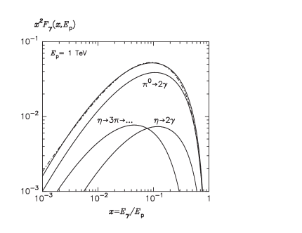
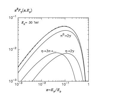
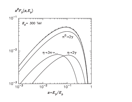
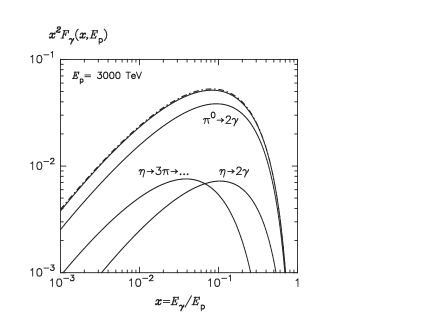
Figure 6: Energy spectra of gamma-rays from pp interactions corresponding to four different energies of incident protons: (a) 1 TeV, (b) 30 TeV, (c) 300 TeV, (d) 3000 TeV. Solid lines - numerical calculations based on simulations of production of $\pi$ and $\eta$ mesons using the SIBYLL code, dot-dashed line - analytical presentation given by Eq.(58). The partial contributions from $\pi^{0}$ and $\eta$ meson decays are also shown.

Eqs.(III.3) – (III.3)

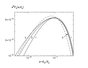
Figure 7: Energy spectra of gamma-rays described by Eq.(58) for three energies of incident protons: 0.1 TeV (curve 1), 100 TeV (curve 2) and 1000 TeV (curve 3). The dashed curve corresponds to the Hillas parameterization of the spectra obtained for proton energies of several tens of TeV.

IV.2 Energy spectra of leptons

The calculations of energy distributions of electrons and neutrinos from p-p have been performed numerically, substituting Eq.(57) into Eqs. (51), (52), and (53). The spectra of electrons from the $\pi\to\mu\,\nu_{\mu}$ decays is well described by the following function

$$F_{e}(x,\,E_{p})=B_{e}\,\frac{(1+k_{e}(\ln x)^{2})^{3}}{x\,(1+0.3/x^{\beta_{e}})}\,(-\ln(x))^{5}\,,$$ (62)

where

$$B_{e} = \frac{1}{69.5+2.65\,L+0.3\,L^{2}}\,,$$ (63)

$$\beta_{e} = \frac{1}{(0.201+0.062\,L+0.00042\,L^{2})^{1/4}}\,,$$ (64)

$$k_{e} = \frac{0.279+0.141\,L+0.0172\,L^{2}}{0.3+(2.3+L)^{2}}\,,$$ (65)

Here $x=E_{e}/E_{\pi}$ and $L=\ln(E_{p}/1\,{\rm TeV})$.

The spectrum of muonic neutrino from the decay of muon, $F_{\nu_{\mu}^{(2)}}(x,\,E_{p})$, is described by the same function; in this case $x=E_{\nu_{\mu}}/E_{p}$.

The spectrum of muonic neutrino produced through the direct decays $\pi\to\mu\,\nu_{\mu}$ can be described as

$$F_{\nu_{\mu}^{(1)}}(x,\,E_{p})=B^{\prime}\,\frac{\ln(y)}{y}\left(\frac{1-y^{\beta^{\prime}}}{1+k^{\prime}y^{\beta^{\prime}}(1-y^{\beta^{\prime}})}\right)^{4}\times$$

$$\left[\frac{1}{\ln(y)}-\frac{4\beta^{\prime}y^{\beta^{\prime}}}{1-y^{\beta^{\prime}}}-\frac{4k^{\prime}\beta^{\prime}y^{\beta^{\prime}}(1-2y^{\beta^{\prime}})}{1+k^{\prime}y^{\beta^{\prime}}(1-y^{\beta^{\prime}})}\right],$$ (66)

where $x=E_{\nu_{\mu}}/E_{p}$, $y=x/0.427$,

$$B^{\prime}=1.75+0.204\,L+0.010\,L^{2}\,,$$ (67)

$$\beta^{\prime}=\frac{1}{1.67+0.111\,L+0.0038L^{2}}\,,$$ (68)

$$k^{\prime}=1.07-0.086\,L+0.002\,L^{2}\,.$$ (69)

The spectrum of $F_{\nu_{\mu}^{(1)}}$ sharply cutoffs at $x=0.427$. The total spectrum of muonic neutrinos $F_{\nu_{\mu}}=F_{\nu_{\mu}^{(1)}}+F_{\nu_{\mu}^{(2)}}$, where $F_{\nu_{\mu}^{(1)}}=F_{e}$. Also, with good accuracy (less than 5%) $F_{\nu_{e}}\approx F_{e}$.

The spectra of electrons and muonic neutrinos for different energies of protons (0.1, 100, and 1000 TeV) are shown in Figs. 8 and 9, respectively.

Although $\pi^{\pm}$-decays strongly dominate in the lepton production (see e.g. Gaisser ), the contribution through decays of other unstable secondaries, first of all K-mesons, is not negligible. In particular, calculations based on simulations of all relevant channels using the SIBYLL code show that the total yield of electrons and neutrinos exceeds Eq.(62) by approximately 10 % at $x\sim 0.1$. At very small values of $x$ the difference increases and could be as large as 20 % at $x\ll 0.1$; at very large values of x, $x\geq 0.5$, it is reduced to 5 %. Thus, for power-law energy distributions of protons, Eqs.(62) and (66) underestimate the flux of neutrinos and electrons by a factor of 1.1. For production of gamma-rays, the simulations performed with the SIBYLL code show that the combined contribution from $\pi^{0}$ and $\eta$ meson decays exceeds 95 % of the total gamma-ray production rate.

To compare the contributions of the final products of decays, in Fig. 10 we show the spectra of gamma-rays, electrons and muonic neutrinos for two energies of incident protons, $E_{p}=0.1$ and 1000 TeV. It is interesting that for significantly different energies of primary protons the spectra of all secondary products are rather similar, although not identical. This explains why for broad and smooth (e.g. power-law type) energy distribution of protons the so-called delta-functional approach of calculating gamma-ray spectra gives quite accurate results (e.g. AhAt00 ; Torres ). However for proton spectra with distinct spectral features, like sharp pileups or cutoffs, this method may lead to wrong conclusions concerning, in particular, the predictions of the energy spectra of gamma-rays and neutrinos.

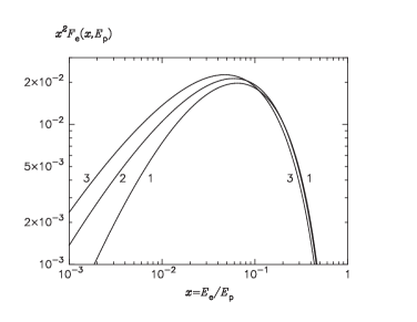
Figure 8: Energy spectra of electrons described by Eq.(62) for three energies of incident protons: 0.1 TeV (curve 1), 100 TeV (curve 2) and 1000 TeV (curve 3).

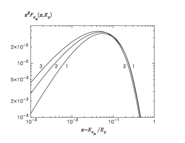
Figure 9: Energy spectra of all muonic neutrinos described by Eq.(62) and (66) for three energies of incident protons: 0.1 TeV (curve 1), 100 TeV (curve 2) and 1000 TeV (curve 3).

 

Figure 10: Energy spectra of all decay products produced at p-p interactions for two energies of incident protons: (a) 0.1 TeV and (b) 1000 TeV. The spectrum of electronic neutrinos is not shown because it practically coincides with the spectrum of electrons.

V Production rates and spectra of photons and leptons for wide energy distributions of protons

The simple analytical approximations presented in the previous section for the energy spectra of secondary particles produced by a proton of fixed energy make the calculations of production rates and spectra of gamma-rays and leptons for an arbitrary energy distribution of protons quite simple. Below we assume that the gas density as well as the magnetic of the ambient medium are sufficiently low, so all secondary products decay before interacting with the gas and the magnetic field.

Let denote by

$$dN_{p}=J_{p}(E_{p})\,dE_{p}$$ (70)

the number of protons in a unite volume in the energy interval $(E_{p},\,E_{p}+dE_{p})$. Below for the function $J_{p}(E_{p})$ we will use units ${\rm cm}^{-3}\,{\rm TeV}^{-1}$. Then the function

$$\Phi_{\gamma}(E_{\gamma})\equiv\displaystyle\frac{dN_{\gamma}}{dE_{\gamma}}=$$

$$\displaystyle c\,n_{H}\int\limits_{E_{\gamma}}^{\infty}\!\sigma_{\rm inel}(E_{p})\,J_{p}(E_{p})\,F_{\gamma}\!\left(\frac{E_{\gamma}}{E_{p}},\,E_{p}\right)\frac{dE_{p}}{E_{p}}\,.$$ (71)

describes the gamma-ray production rate in the energy interval $(E_{\gamma},\,E_{\gamma}+dE_{\gamma})$, where $n_{H}$ is the density of the ambient hydrogen gas, $\sigma_{\rm inel}(E_{p})$ is the cross-section of inelastic p-p interactions, and $c$ is the speed of light. The function $F_{\gamma}(x,\,E_{p})$ is defined by Eq.(58). For the variable $x=E_{\gamma}/E_{p}$ Eq.(71) can be written in the following form

$$\Phi_{\gamma}(E_{\gamma})=$$

$$\displaystyle c\,n_{H}\int\limits_{0}^{1}\!\sigma_{\rm inel}(E_{\gamma}/x)\,J_{p}(E_{\gamma}/x)\,F_{\gamma}(x,\,E_{\gamma}/x)\,\frac{dx}{x}\,.$$ (72)

Analogous equations describe the production of neutrinos $\nu+\tilde{\nu}$ and electrons $e^{-}+e^{+}$; for muonic neutrinos both contributions from Eqs.(62) and (66) should be included in calculations. The inelastic part of the total cross-section of p-p interactions $\sigma_{\rm inel}(E_{p})$ can be presented in the following form

$$\sigma_{\rm inel}(E_{p})=34.3+1.88\,L+0.25\,L^{2}\,,\;{\rm mb}\,,$$ (73)

where $L=\ln(E_{p}/1\,{\rm TeV})$. This approximation is obtained with the fit of the numerical data included in the SIBYLL code.

Thus, the calculation of production rates of gamma-rays, electrons and neutrinos for an arbitrary energy distribution of protons is reduced to one-dimensional integrals like the one given by Eq.(72). The analytical presentations described in the previous section can be used, however, only at high energies: $E_{p}>0.1\,{\rm TeV}$, and $x_{i}=E_{i}/E_{p}\geq 10^{-3}$. Continuation of calculations to lower energies requires a special treatment which is beyond the scope of this paper. This energy region has been comprehensively studied by Dermer Dermer86 and recently by Kamae et al. Kamae05 . On the other hand one may suggest a simple approach which would allow to continue the calculations, with a reasonable accuracy, down to the threshold energies of production of particles at pp interactions. In particular, for distributions of protons presented in the form

$$J_{p}(E_{p})=\frac{A}{E_{p}^{\alpha}}\,\exp\left[-\left(\frac{E_{p}}{E_{0}}\right)^{\beta}\right]\,,$$ (74)

the spectra of gamma-rays and other secondaries can be continued to low energies using the $\delta$-functional approximation as proposed in Ref.AhAt00 . We suggest a modified version of this approach. Namely, we adopt for the production rate of $\pi$-mesons

$$\tilde{F}_{\pi}=\tilde{n}\,\delta\left(E_{\pi}-\frac{\kappa}{\tilde{n}}\,E_{\rm kin}\right),$$ (75)

where $E_{\rm kin}=E_{p}-m_{p}$ is the kinetic energy of protons. The physical meaning of parameters $\tilde{n}$ and $\kappa$ is clear from the following relations:

$$\int\!\tilde{F}_{\pi}\,dE_{\pi}=\tilde{n}\,,\quad{\rm and}\quad\int\!E_{\pi}\,\tilde{F}_{\pi}\,dE_{\pi}=k\,E_{\rm kin}\,.$$ (76)

$\tilde{n}$ is the number of produced pions for the given distribution function $\tilde{F}_{\pi}$, and $\kappa$ is the fraction of kinetic energy of the proton transferred to gamma-rays or leptons. For example for power-law type distribution functions $\tilde{F}_{\pi}(E)\propto E^{-\alpha}$ with $\alpha\geq 2$, the parameter $\tilde{n}\sim 1$.

Assuming that the parameters $\tilde{n}$ and $\kappa$ depend weakly on the proton energy, from Eq.(75) one finds the production rate of $\pi^{0}$-mesons

$$q_{\pi}(E_{\pi})=\tilde{n}\,\frac{c\,n_{H}}{K_{\pi}}\,\sigma_{\rm inel}\!\left(m_{p}+\frac{E_{\pi}}{K_{\pi}}\right)J_{p}\!\left(m_{p}+\frac{E_{\pi}}{K_{\pi}}\right),$$ (77)

where $K_{\pi}=\kappa/\tilde{n}$. For the procedure described below $\tilde{n}$ and $K_{\pi}$ are free parameters.

The emissivity of gamma-rays is related to $q_{\pi}(E_{\pi})$ though the equation

$$\frac{dN_{\gamma}}{dE_{\gamma}}=2\int\limits_{E_{\min}}^{\infty}\frac{q_{\pi}(E_{\pi})}{\sqrt{E_{\pi}^{2}-m_{\pi}^{2}}}\,dE_{\pi}\,,$$ (78)

where $E_{\min}=E_{\gamma}+m_{\pi}^{2}/4E_{\gamma}$.

The feasibility of the $\delta$-functional approximation in the energy range $E<100\,{\rm GeV}$ is explained by the following reasons.

1. In the energy range $1\ll E\lesssim 100\,{\rm GeV}$ the cross-section given by Eq.(73) is almost constant, and the spectrum of protons given by Eq.(74) has a power-law form. Therefore the spectra of gamma-rays and leptons are also power-law with the same index $\alpha$. In this case the $\delta$-functional approximation leads to power-law spectra for any choice of parameters $\tilde{n}$ and $K_{\pi}$. Therefore for the given $K_{\pi}$ and defining the value of $\tilde{n}$ from the condition of continuity of the spectrum at the point $E=100\,{\rm GeV}$, one can obtain correct dependence and absolute value of the gamma-ray spectrum at $1\ll E\lesssim 100\,{\rm GeV}$.

2. For the value of $K_{\pi}=0.17$, the $\delta$-functional approximation for power-law proton spectra agrees quite well, as is demonstrated in Ref.AhAt00 , with numerical Monte Carlo calculations Mori , even at energies as low as $E\sim 1\;{\rm GeV}$ (see also discussion in Torres ). At lower energies one has to use, instead of Eq. (73), a more accurate approximation for the inelastic cross-section:

$$\sigma_{\rm inel1}(E_{p})=(34.3+1.88\,L+0.25\,L^{2})\,\times$$

$$\displaystyle\left[1-\left(\frac{E_{th}}{E_{p}}\right)^{\!\!4}\right]^{2}\,,\;{\rm mb}\,,$$ (79)

where $E_{th}=m_{p}+2m_{\pi}+m_{\pi}^{2}/2m_{p}=1.22\cdot 10^{-3}\,{\rm TeV}$ is the threshold energy of production of $\pi^{0}$-mesons. Eq.(79) correctly describes the cross-section also at energies close to the threshold, and at $E_{p}>3\,E_{th}$ almost coincides with Eq.(73). The comparison with experimental data ParticleData shows that Eq.(79) can be used in wider energy range of protons, as it is demonstrated in Fig. 11.

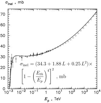
Figure 11: Inelastic cross-secton of p-p interactions approximated by Eq.(79). The experimental data are from http:wwwppds.ihep.su:8001/c5-5A.HTML, the open points correspond to the cross-sections which are used in the SIBYLL code.

In Fig. 12 we show the spectra of gamma-rays and leptons calculated for the proton distribution given by Eq.(74). The constant $A$ is determined from the condition

$$\int_{1\,{\rm TeV}}^{\infty}E_{p}\,J_{p}(E_{p})\,dE_{p}=1\;{\rm erg}\;{\rm cm}^{-3}\,.$$ (80)

In the energy range $E\geq 0.1\;{\rm TeV}$ calculations are performed using Eq. (72) with functions $F_{j}(x,\,E_{p})$ presented in Section IV; at lower energies the $\delta$-functional approximation is used with $K_{\pi}=0.17$. As discussed above, $\tilde{n}$ is treated as a free parameter determined from the condition to match the spectrum based on accurate calculations at $E=0.1\,{\rm TeV}$. The parameter $\tilde{n}$ depends on the spectrum of primary protons. For example, for gamma-rays, $\tilde{n}=1.10$; 0.86, and 0.91 for power-law proton spectra with $\alpha=2\,;$ 2.5, and 3, respectively. For electrons these numbers are somewhat different, namely $\tilde{n}=0.77$; 0.62, and 0.67 for the same spectral indices of protons.

In In Fig. 12 we show also the gamma-ray spectrum obtained with the $\delta$-functional approximation in the entire energy range (dashed line). At low energies where the gamma-ray spectrum behaves like power-law, the $\delta$-functional approximation agrees very well with accurate calculations. However in the high energy regime where the proton spectrum deviates from power-law, the $\delta$-functional approximation fails to describe correctly the gamma-ray spectrum.

It should be noted that the noticeable spectral feature (hardening) around $E\sim 0.1\;{\rm TeV}$ in Fig. 12a is not a computational effect connected with the transition from the $\delta$-functional approximation at low energies to accurate calculations at higher energies. This behavior is caused, in fact, by the increase of the cross-section $\sigma_{\rm inel}$ which becomes significant at energies of protons above 1 TeV (see Fig. 11). This is demonstrated in Fig. 13. Indeed, it can be seen that under a formal assumption of energy-independent cross-section, $\sigma_{\rm inel}={\rm const}$, the effect of the spectral hardening disappears.

One can seen from Figs. 12a,b that the exponential cutoff in the spectrum of protons at $E_{0}=10^{3}$ TeV has an impact on the spectrum of gamma-rays already at 10 TeV, i.e. as early as $0.01E_{0}$. The reason for such an interesting behavior can be understood from the following qualitative estimates. The integrand of Eq.(72) at $E_{\gamma}\ll E_{0}$ has sharp maximum in the region of small $x$. To find the location of the maximum, let’s assume $\sigma_{\rm inel}={\rm const}$, and replace the distribution $F_{\gamma}$ from Eq.(58) by a model function $F_{\gamma}\propto(1-x)^{4}/x$ which correctly describes the features of $F_{\gamma}$ at points $x=0$ and $x=1$. Then for $\alpha=2$ and $\beta=1$ the integrand is proportional to the following function

$$g(x)=(1-x)^{4}\,e^{-\rho/x}\,,$$ (81)

where $\rho=E_{\gamma}/E_{0}$. Presenting the function $g(x)$ in the form $g(x)=\exp[h(x)]$, one can estimate the integral of this function using the saddle-point integration method,

$$\int\limits_{0}^{1}\!g(x)\,dx\sim\exp[h(x_{*})]\ ,$$ (82)

where $x_{*}=\frac{1}{8}\,(\sqrt{\rho^{2}+16\rho}-\rho)$ is the location of the maximum of the function $h(x)$. At $\rho\lesssim 1$ one has $h(x_{*})\approx-4\,\rho^{1/2}-\rho/2$. Therefore the spectrum of gamma-rays contains an exponential term $\exp\left[-(16\,E_{\gamma}/E_{0})^{1/2}\right]$. The impact of this term is noticeable already at energies $E_{\gamma}\gtrsim 10^{-2}\,E_{0}$. This formula also shows that the spectrum of gamma-rays decreases slower compared to the spectrum of parent protons. In the $\delta$-functional approximation the gamma-ray spectrum repeats the shape of the proton spectrum. The deviation of the $\delta$-functional approximation from the correct description of the gamma-ray spectrum is clearly seen in Figs.12a,b.

Finally we note that for $\alpha=2$ and at energies $E\ll E_{0}$, the amplitide of the gamma-ray spectrum exceeds the level of the flux of muonic neutrinos. The difference is due to the additional contribution of $\eta$-mesons in production of gamma-rays. If one takes into account only gamma-rays from decays of $\pi^{0}$-mesons, the spectra of gamma-rays and muonic neutrinos are almost identical at energies well below the cutoff region, where both have power-law behavior. This conclusion is in good agreement with early studies Berez91 ; Gaisser ; DAV ; Vissani , and does not contradict to the fact that in each pp interaction the number of muonic neutrinos is a factor of 2 larger, on average, than the number of gamma-rays. The disbalance is compensated, in fact, at low energies. In Fig. 14 we show spectra of photons and leptons at very low energies (see Section III). It is seen that the number of muonic neutrinos indeed significantly exceeds the number of gamma-rays.

Figure 12: Energy spectra of gamma-rays and leptons from p-p interactions calculated for the distribution of protons given by Eq.(74) with parameters $E_{0}=$1000 TeV, $\beta=1$ and (a) $\alpha=2$, (b)$\alpha=1.5$. The dashed curves are calculated in the $\delta$-functional approximation.

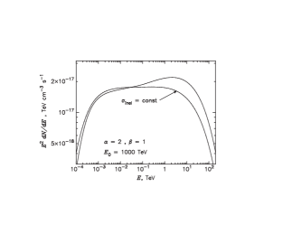
Figure 13: Comparison of energy spectra of gamma-rays calculated for the nominal inelastic cross-section given by Eq.(73) and a formally assumed energy independent cross-section $\sigma_{\rm inel}=34\,{\rm mb}$. The proton distribution is given by Eq.(74), the relevant parameters are shown in figure.

Figure 14: Energy spectra of gamma-rays and leptons from pp interactions in the very low energy band. The energy distribution of parent protons is given by Eq.(74), the relevant parameters $\alpha$, $\beta$, $E_{0}$ are shown in figures.

VI Summary

We present new parameterizations of energy spectra of gamma-rays, electrons and neutrinos produced in proton-proton collisions. The results are based on the spectral fits of secondaries produced in inelastic p-p interactions simulated by the SIBYLL code. The recommended simple analytical presentations provide accuracy better than 10 percent over the energy range of parent protons $0.1-10^{5}$ TeV and $x=E_{i}/E_{p}\geq 10^{-3}$.

Appendix A Energy distributions of neutrinos and electrons from decays of charged pions

For derivation of the energy distributions of electrons and neutrinos at decays of charged pions, below we introduce three systems of reference – $K^{\prime}$, $K_{0}$, and $K$ corresponding to the the muon rest system, the pion rest system and the laboratory system, respectively. For certainty, we will consider the $\pi^{-}$-decay Since $m_{\mu}\gg m_{e}$ we will neglect the mass of the electron.

Let’s denote by $g_{e}(E^{\prime}_{e},\cos\tilde{\theta}^{\prime})\,dE^{\prime}_{e}\,d\Omega^{\prime}$ the energy and and angular distribution of electrons in the system $K^{\prime}$, where $\tilde{\theta}^{\prime}$ – is the angle between the muon spin and the electron momentum. Since at the $\pi^{-}$ decay the muon’s spin is parallel to its momentum, for derivation of the distribution in the $K_{0}$ system one needs to perform Lorentz transformation towards the muon’s spin. This results in

$$g^{(0)}_{e}(E_{e0},\cos\theta_{0})\,dE_{e0}\,d\Omega_{0}=\frac{1}{\gamma_{\mu}(1-\beta_{\mu}\cos\theta_{0})}\times$$

$$g_{e}\!\left(E_{e0}\gamma_{\mu}(1-\beta_{\mu}\cos\theta_{0}),\,\frac{\cos\theta_{0}-\beta_{\mu}}{1-\beta_{\mu}\cos\theta_{0}}\right)dE_{e0}\,d\Omega_{0}\,,$$ (83)

where $E_{e0}$ is the energy of the electron, $\theta_{0}$ is the angle between the electron and muon momenta, and

$$\gamma_{\mu}=\frac{1+r}{2\sqrt{r}}\,,\quad\beta_{\mu}=\frac{1-r}{1+r}\,,$$ (84)

are the Lorentz factor and speed of the muon - all in the $K_{0}$ system; $r=m_{\mu}^{2}/m_{\pi}^{2}$.

In the $K_{0}$ system the muon can be emitted, with same probability, at any angle, therefore Eq.(83) should be averaged over the muon directions. The function $g_{e}$ is given by Eq.(31) in Sec.III. Then, denoting $\cos\theta_{0}={\bf n}_{e}{\bf n}_{\mu}$ (${\bf n}_{e}$ and ${\bf n}_{\mu}$ – are unite vectors towards the electron and muon momenta), and integrating over the directions of the vector ${\bf n}_{\mu}$, one obtains

$$\bar{g}_{e0}(E_{e0})\,dE_{e0}\,d\Omega_{0}=F_{e}(\xi)\;d\xi\,\frac{d\Omega_{0}}{4\pi}\,.$$ (85)

Here

$$F_{e}(\xi)=\Psi_{e}^{(1)}(\xi)\,\Theta(r-\xi)+\Psi_{e}^{(2)}(\xi)\,\Theta(\xi-r)\,,$$ (86)

where $\xi=2E_{e0}/m_{\pi}$ varies within $0\leq\xi\leq 1$, and

$$\Psi_{e}^{(1)}(\xi)=\frac{2\xi^{2}}{3r^{2}}\,(3+6r-2\xi-4r\xi)\,,$$ (87)

$$\Psi_{e}^{(2)}(\xi)=\frac{2\,(3-2r-9\xi^{2}+6r\xi^{2}+6\xi^{3}-4r\xi^{3})}{3(1-r)^{2}}\,.$$ (88)

The spherically symmetric function given by Eq.(85) describes the energy and angular distribution of electrons in the pion rest system.

Similar calculations for electronic neutrinos result in

$$\bar{g}_{\nu_{e}0}(E_{e0})\,dE_{\nu_{e}0}\,d\Omega_{0}=F_{\nu_{e}}(\xi)\;d\xi\,\frac{d\Omega_{0}}{4\pi}\,.$$ (89)

In this equation $\xi=2E_{\nu_{e}}/m_{\pi}$ ($0\leq\xi\leq 1$), and

$$F_{\nu_{e}}(\xi)=\Psi_{\nu_{e}}^{(1)}(\xi)\,\Theta(r-\xi)+\Psi_{\nu_{e}}^{(2)}(\xi)\,\Theta(\xi-r)\,,$$ (90)

where

$$\Psi_{\nu_{e}}^{(1)}(\xi)=\frac{4\xi^{2}}{r^{2}}\,(3r-\xi-2r\xi)\,,$$ (91)

$$\Psi_{\nu_{e}}^{(2)}(\xi)=\frac{4\,(-r+3\xi-6\xi^{2}+3r\xi^{2}+3\xi^{3}-2r\xi^{3})}{(1-r)^{2}}\,.$$ (92)

Now one can calculate, for the distributions of electrons and neutrinos in the $K_{0}$ system given by Eqs.(85) and (89), the corresponding energy distributions in the Laboratory system $K$. Generally, the exact analytical presentations of these distributions appear quite complex, therefore in Sec.III we present Eqs.(III.3) – (III.3) derived for the most interesting case of ultrarelativistic pions.

Finally we should note that the energy distributions of electrons published in Ref.Mosk are not correct. From derivation of Eq.(C2) of that paper one can conclude that this equation is obtained under the assumption that the muon and pion momenta are strictly parallel, i.e. the important step of integration of Eq.(C2) over the muon directions was erroneously skipped. Consequently, the integration of Eq.(C2) over the energy distribution of muons leads to inaccurate Equations (C6) - (C12) of Ref.Mosk .

References

- (1) P. Morrison, Nuovo Cimento 7, 858 (1957).
- (2) V.L. Ginzburg and S.I. Syrovatskii, Origin of Cosmic Rays, New York: Macmillan (1964).
- (3) S. Hayakawa, Cosmic RayPhysics, New York: Wiley (1964).
- (4) F.W. Stecker, Cosmic gamma rays, Baltimore: Mono Book Corp. (1971).
- (5) V.S. Berezinsky, V.V.Volynsky, in Proc. 16th ICRC, Kyoto, 1979, vol. 10, p. 326; p.332.
- (6) S.A. Stephens and G.D. Badhwar, Astrophys. Space Sci. 76, 213 (1981).
- (7) C.D. Dermer, Astron. Astrophys. 157, 223 (1981).
- (8) V.S. Berezinsky, S.V. Bulanov, V.A. Dogiel, V.L. Ginzburg and S.V. Ptuskin, Astrophysics of Cosmic Rays, Amsterdam: North-Holland (1990).
- (9) T.K. Gaisser, Cosmic Rays and Particle Physics, Cambridge: Cambridge University Press (1990).
- (10) V.S. Berezinsky, Nucl. Phys B Proc Suppl 19, 375 (1991).
- (11) M.L. Costantini and F. Vissani, Astroparticle Physics 23, 477 (2005).
- (12) M. Mori, ApJ 478, 225 (1997).
- (13) F.A. Aharonian and A.M. Atoyan, Astron. Astrophys. 362, 937 (2000).
- (14) A.W. Strong, I.V. Moskalenko, O. Reimer ApJ 537, 763 (2000).
- (15) T. Kamae, T. Abe, T. Koi 2005, ApJ 620, 244 (2005); T. Kamae, N. Karlsson, T. Misuno, T. Abe, T. Koi 2006, submitted to ApJ, (astro-ph/0605581)
- (16) E. Domingo-Santamaria, D. Torres, Astron. Astrophys., in press (astro-ph/0506240).
- (17) T. Sjöstrand, L. Lonnblad, S. Mrenna, Pythia 6.2: Physics and Manual (hep-ph/0108264), 2001.
- (18) R.S. Fletcher, T.K. Gaisser, P. Lipari and T. Stanev, Phys. Rev. D50, 5710 (1994).
- (19) N.N. Kalmykov, S.S. Ostapchenko, A.I. Pavlov 1997, Nucl. Phys. Proc. Suppl. B52, 17 (1997).
- (20) D. Heck, J. Knapp 2003, Extensive Air Shower Simulatrion with CORSIKA: A user’s Guide (v. 6.020, KZK Report, Feb 18, 2003).
- (21) S.R. Blattnig, R. Swaminathan, A.T. Kruger, M. Ngom, J.N. Norbury, Phys ReV 62, 094030 (2000).
- (22) P. Lipari, Astroparticle Physics 1, 195 (1993).
- (23) L.B. Okun, Weak interaction of elementary particles, New York: Pergamon Press (1965).
- (24) I.V. Moskalenko, A.W. Strong, ApJ 493, 694 (1998).
- (25) A. M. Hillas, J. Phys. G: Nucl. Part. Phys. 31, R95 (2005).
- (26) S. Eidelman et al., Review of Particle Physics, Phys. Lett. B592, 1 (2004).
- (27) L.O’C. Drury, F.A. Aharonian, H.J. Völk, Astron. Astrophys. 287, 959 (1994).