Observations of the Hot Horizontal-Branch Stars in the Metal-Rich Bulge Globular Cluster NGC 6388

The metal-rich bulge globular cluster NGC 6388 shows a distinct blue horizontal-branch tail in its colour-magnitude diagram (Rich et al. 1997) and is thus a strong case of the well-known 2^nd Parameter Problem. In addition, its horizontal branch (HB) shows an upward tilt toward bluer colours, which cannot be explained by canonical evolutionary models. Several noncanonical scenarios have been proposed to explain these puzzling observations. In order to test the predictions of these scenarios, we have obtained medium resolution spectra to determine the atmospheric parameters of a sample of the blue HB stars in NGC 6388. Using the medium resolution spectra, we determine effective temperatures, surface gravities and helium abundances by fitting the observed Balmer and helium lines with appropriate theoretical stellar spectra. As we know the distance to the cluster, we can verify our results by determining masses for the stars. During the data reduction we took special care in subtracting the background, which is dominated by the overlapping spectra of cool stars. The cool blue tail stars in our sample with effective temperatures ${\rm T_{eff}}$ $\approx$ 10,000 K have lower than canonical surface gravities, suggesting that these stars are, on average, ${\approx}$0$\aas@@fstack{m}$4 brighter than canonical HB stars in agreement with the observed upward slope of the HB in NGC 6388. Moreover, the mean mass of these stars agrees well with theoretical predictions. In contrast, the hot blue tail stars in our sample with ${\rm T_{eff}}$ $\geq$ 12,000 K show significantly lower surface gravities than predicted by any scenario, which can reproduce the photometric observations. Their masses are also too low by about a factor of 2 compared to theoretical predictions. The physical parameters of the blue HB stars near 10,000 K support the helium pollution scenario. The low gravities and masses of the hot blue tail stars, however, are probably caused by problems with the data reduction, most likely due to remaining background light in the spectra, which would affect the fainter hot blue tail stars much more strongly than the brighter cool blue tail stars. Our study of the hot blue tail stars in NGC 6388 illustrates the obstacles which are encountered when attempting to determine the atmospheric parameters of hot HB stars in very crowded fields using ground-based observations. We discuss these obstacles and offer possible solutions for future projects.

1 Introduction

Ever since its discovery over 30 years ago (Sandage & Wildey sawi67 (1967); van den Bergh vdbe67 (1967)), the 2^nd parameter effect has stood as one of the major unsolved challenges in the study of the Galactic globular clusters. While it was recognized quite early that the horizontal branch (HB) becomes redder on average with increasing metallicity, many pairs of globular clusters are known with identical metallicities but markedly different HB morphologies, e.g., M 3 versus M 13. Thus some parameter(s) besides metallicity (the 1^st parameter) must affect the evolution of the HB stars in these globular clusters. Possible 2^nd parameter candidates include the globular cluster age, mass loss along the red-giant branch (RGB), helium abundance $Y$, $\alpha$-element abundance, cluster dynamics, stellar rotation, deep mixing, etc.

Hubble Space Telescope observations by Rich et al. (riso97 (1997)) have found an unexpected population of hot HB stars in the metal-rich globular clusters NGC 6388 and NGC 6441 ([Fe/H] $\approx-0.5$), making these clusters the most metal-rich clusters to show the 2^nd parameter effect. Ordinarily metal-rich globular clusters have only a red HB clump. However, NGC 6388 and NGC 6441 possess extended blue HB tails containing ${\approx}15$% of the total HB population. Quite remarkably, the HBs in both clusters slope upward with decreasing $B-V$ with the stars at the top of the blue tail being nearly 0$\aas@@fstack{m}$5 brighter in $V$ than the well-populated red HB clump. Moreover, the RR Lyrae variables in these clusters have unusually long periods for the cluster metallicity, leading Pritzl et al. (prsm00 (2000)) to suggest that NGC 6388 and NGC 6441 may represent a new Oosterhoff group. For all of these reasons the HBs of NGC 6388 and NGC 6441 are truly exceptional.

In the next section we will discuss the implications of NGC 6388 and NGC 6441 for the 2^nd parameter effect and will review a number of scenarios for explaining the HB morphology of these clusters. Sect. 3 describes the observations and reduction of the medium resolution spectra that we have obtained to test these scenarios, while Sect. 4 gives the atmospheric parameters derived from these spectra. These results are compared with the theoretical HB tracks in Sect. 5. Sect. 6 summarizes our conclusions.

2 Horizontal-Branch Morphology: Problems and Scenarios

The presence of hot HB stars in globular clusters as metal-rich as NGC 6388 and NGC 6441 may provide an important diagnostic for understanding the 2^nd parameter effect for the following reason. In intermediate-metallicity globular clusters such as M 3 the HB spans a wide range in color that extends both blueward and redward of the instability strip. The location of a star along the HB is then quite sensitive to changes in the stellar parameters. In fact, this is why the HB is “horizontal”. In metal-rich globular clusters, however, the situation is different. Due to their high envelope opacity, metal-rich HB stars are normally confined to a red clump. To move such stars blueward requires a larger change in the stellar structure than for intermediate-metallicity stars. Thus any 2^nd parameter candidate capable of producing hot HB stars in a metal-rich globular cluster might also have other observational consequences. Indeed, the upward sloping HBs in NGC 6388 and NGC 6441 suggest that the 2^nd parameter in these globular clusters is affecting both the temperature and the luminosity of the HB stars.

Can canonical models explain the upward sloping HBs in NGC 6388 and NGC 6441? In principle, one could produce hot HB stars in these globular clusters by increasing the cluster age or by enhancing the amount of mass loss along the RGB. Rich et al. (riso97 (1997)) considered both of these possibilities but found neither of them to be satisfactory because the required increase in the cluster age is quite large and because the frequency of stellar interactions within the cores of these clusters seems too low to produce the additional RGB mass loss. This conclusion was further supported by the theoretical HB simulations of Sweigart & Catelan (swca98 (1998), hereafter SC98). They found that the HB morphology predicted by canonical HB models is flat in the (${M_{V}}$, $B-V$) plane. Increasing the cluster age or the RGB mass loss simply moves the models blueward in $B-V$ without increasing their luminosity. Thus canonical HB models cannot account for the HB morphology of NGC 6388 and NGC 6441. In particular, two of the most prominent 2^nd parameter candidates – age and RGB mass loss – do not work.

More recently, Raimondo et al. (raca02 (2002)) have argued that canonical HB models can produce upward sloping HBs if the metallicity is sufficiently high or if the mixing-length ratio $\alpha$ describing the superadiabatic convection in the outer layers of the red HB stars is sufficiently small. Their solar metallicity models with $\alpha$ = 1.0 predict a luminosity difference $\Delta V$ between the top of the blue tail and the red HB clump that exceeds the 0$\aas@@fstack{m}$5 observed in NGC 6388 and NGC 6441. However, such a small value for the mixing-length ratio is untenable because it would imply a $B-V$ colour for the RGB that is much redder than observed. The predicted $\Delta V$ for the more appropriate mixing-length ratio $\alpha$ = 1.6 is only ${\approx}$ 0$\aas@@fstack{m}$2 for a solar metallicity and decreases further with decreasing [Fe/H]. At the metallicity of NGC 6388 and NGC 6441 the Raimondo et al. models predict little difference in the luminosity of HB stars at the top of the blue tail compared to those in the red clump, further confirming that some noncanonical effect must be influencing the HB morphology in NGC 6388 and NGC 6441.

The failure of canonical HB models to produce upward sloping HBs has prompted the study of other noncanonical solutions. Theoretical models show that the HB luminosity at a fixed metallicity depends on two parameters: the helium abundance $Y$ and the core mass ${M_{c}}$. This fact lead SC98 to suggest 3 noncanonical scenarios involving increases in either $Y$ or ${M_{c}}$ which might potentially produce upward sloping HBs.

The first (“high-$Y$”) scenario assumes that the stars in NGC 6388 and NGC 6441 formed with a high primordial helium abundance due to a peculiar chemical enrichment history in these clusters. From theoretical models we know that HB tracks at high helium abundances have very long blue loops which deviate considerably from the zero-age HB (ZAHB). The HB simulations of SC98 show that such high-$Y$ tracks can indeed produce upward sloping HBs as seen in NGC 6388 and NGC 6441 provided $Y$ is very large ($\stackrel{{\scriptstyle>}}{{\scriptstyle\sim}}$ 0.4). However, this scenario predicts too large a value for the number ratio $R$ of HB stars to RGB stars brighter than the HB (Layden et al. lari99 (1999)) as well as too bright a luminosity for the RGB bump (Raimondo et al. raca02 (2002)). Thus a high primordial helium abundance in NGC 6388 and NGC 6441 can be ruled out.

The second (“rotation”) scenario is based on the fact that internal rotation within an RGB star can delay the helium flash, thereby leading to a larger core mass and greater mass loss near the tip of the RGB. This increase in the core mass ${M_{c}}$ together with the corresponding decrease in the total mass $M$ will shift a star’s HB location towards higher effective temperatures and luminosities. HB simulations show that this scenario can also produce upward sloping HBs similar to those observed in NGC 6388 and NGC 6441. However, it is difficult to understand how the blue HB stars in NGC 6388 and NGC 6441 could have the high rotation rates required by this scenario. Preliminary results from high resolution spectra of three cool blue HB stars (${\rm T_{eff}}$ $\lesssim$ 10,000 K) in NGC 6388 do not show evidence for rotation velocities of $v\sin i\gtrsim 10$ km sec^-1 (Moehler & Sweigart mosw06 (2006)). Thus the rotation scenario seems unlikely.

The third (“helium-mixing”) scenario is motivated by the large star-to-star abundance variations which are found among the red-giant stars within individual globular clusters and which are sometimes attributed to the mixing of nuclearly processed material from the vicinity of the hydrogen shell out to the stellar surface (Kraft kraf94 (1994)). The observed enhancements in Al are particularly important because they would require the mixing to penetrate deeply into the hydrogen shell (Cavallo et al. casw98 (1998)). Such mixing would dredge up fresh helium together with Al, thereby increasing the envelope helium abundance and leading to a brighter RGB tip luminosity and hence greater mass loss. Thus a helium-mixed star would arrive on the HB with both a higher envelope helium abundance and a lower mass and would therefore be both bluer and brighter than its canonical counterpart - just what is needed to produce an upward sloping HB. Indeed, the HB simulations of SC98 confirm that helium mixing can produce HB morphologies similar to those in NGC 6388 and NGC 6441. However, the existence of helium mixing on the RGB can be questioned on several grounds. The O-Na and Mg-Al anticorrelations observed in turnoff stars of NGC 6752 by Gratton et al. (grbo01 (2001)) indicate that the Al enhancements are more likely due to primordial pollution from an earlier generation of stars than to deep mixing on the RGB. It is also questionable whether the mixing currents could overcome the large gradient in the mean molecular weight within the hydrogen shell of a RGB star. Thus helium mixing also seems unlikely.

These difficulties have prompted a number of additional suggestions for explaining the HB morphologies of NGC 6388 and NGC 6441. One of the earliest suggestions, offered by Piotto et al. (piso97 (1997)), was a spread in metallicity. In this case the blue HB stars would be metal-poor compared to the stars in the red HB clump. Because the HB becomes brighter in $V$ with decreasing metallicity, the blue HB stars would also be brighter. Thus a metallicity spread might also produce an upward sloping HB. This possibility was studied by Sweigart (swei02 (2002)), who showed that upward sloping HBs similar to those in NGC 6388 and NGC 6441 would require the stars at the top of the blue HB tail to be approximately 2 dex more metal-poor than the stars in the red HB clump. However, Raimondo et al. (raca02 (2002)) have noted that the progenitors of the blue HB stars should appear as a population of metal-poor giants lying well to the blue of the metal-rich RGB. Since such metal-poor giants are not seen in the colour-magnitude diagrams of NGC 6388 and NGC 6441, Raimondo et al. (raca02 (2002)) conclude that any metallicity spread must be small. Again preliminary results of the high resolution spectra mentioned above do not show any evidence for a significant metal deficiency in these blue HB stars compared to the overall metallicity of NGC 6388 (Moehler & Sweigart mosw06 (2006)).

Piotto et al. (piso97 (1997)) also suggested that NGC 6388 and NGC 6441 might contain two stellar populations with different ages. This possibility has been further explored by Ree et al. (reyo02 (2002)). Their population models for NGC 6388 and NGC 6441 are able to produce blue HB stars provided these stars are older by 1.2 Gyr and metal-poor by 0.15 dex compared to the stars in the red HB clump. Such a small difference in metallicity between the blue and red HB stars avoids the problem with the missing metal-poor giants discussed above. However, while such models might produce bimodal HBs, they do not produce an upward sloping HB. As shown by SC98, differences in age merely move an HB star horizontally along the HB, and, as shown by Sweigart (swei02 (2002)), a metallicity difference of 0.15 dex is too small to produce a significant HB slope. Thus the Ree et al. (reyo02 (2002)) models do not account for a key property of the HBs in NGC 6388 and NGC 6441. Ree et al. (reyo02 (2002)) also suggest that the long RR Lyrae periods might be explained if these stars are highly evolved from the blue HB. While such stars would be brighter and hence have longer periods, they would also evolve rapidly across the instability strip on their way to the asymptotic-giant branch (AGB). Explaining the observed number of RR Lyrae stars under such a scenario would therefore be very difficult (Pritzl et al. prsm02 (2002)).

Table 1: Coordinates and photometric data for our target stars (from Piotto et al. piso97 (1997))

number	$\alpha_{2000}$	$\delta_{2000}$	$V$	$B-V$	setup
1283	17h36m23$\stackrel{{\scriptstyle\rm s}}{{.}}$899	-44∘44′58$.\!\!{\arcsec}$45	$\rm 18\stackrel{{\scriptstyle m}}{{.}}690$$\pm$$\rm 0\stackrel{{\scriptstyle m}}{{.}}032$	$\rm+0\stackrel{{\scriptstyle m}}{{.}}230$$\pm$$\rm 0\stackrel{{\scriptstyle m}}{{.}}041$	1
1775	17h36m14$\stackrel{{\scriptstyle\rm s}}{{.}}$921	-44∘43′08$.\!\!{\arcsec}$87	$\rm 18\stackrel{{\scriptstyle m}}{{.}}811$$\pm$$\rm 0\stackrel{{\scriptstyle m}}{{.}}040$	$\rm+0\stackrel{{\scriptstyle m}}{{.}}292$$\pm$$\rm 0\stackrel{{\scriptstyle m}}{{.}}047$	1
2612	17h36m22$\stackrel{{\scriptstyle\rm s}}{{.}}$560	-44∘44′01$.\!\!{\arcsec}$93	$\rm 19\stackrel{{\scriptstyle m}}{{.}}622$$\pm$$\rm 0\stackrel{{\scriptstyle m}}{{.}}059$	$\rm+0\stackrel{{\scriptstyle m}}{{.}}279$$\pm$$\rm 0\stackrel{{\scriptstyle m}}{{.}}068$	1
4113	17h36m22$\stackrel{{\scriptstyle\rm s}}{{.}}$884	-44∘44′24$.\!\!{\arcsec}$63	$\rm 16\stackrel{{\scriptstyle m}}{{.}}776$$\pm$$\rm 0\stackrel{{\scriptstyle m}}{{.}}026$	$\rm+0\stackrel{{\scriptstyle m}}{{.}}545$$\pm$$\rm 0\stackrel{{\scriptstyle m}}{{.}}037$	1
6239	17h36m19$\stackrel{{\scriptstyle\rm s}}{{.}}$813	-44∘43′05$.\!\!{\arcsec}$88	$\rm 19\stackrel{{\scriptstyle m}}{{.}}147$$\pm$$\rm 0\stackrel{{\scriptstyle m}}{{.}}036$	$\rm+0\stackrel{{\scriptstyle m}}{{.}}244$$\pm$$\rm 0\stackrel{{\scriptstyle m}}{{.}}041$	1
7104	17h36m17$\stackrel{{\scriptstyle\rm s}}{{.}}$879	-44∘45′05$.\!\!{\arcsec}$02	$\rm 19\stackrel{{\scriptstyle m}}{{.}}310$$\pm$$\rm 0\stackrel{{\scriptstyle m}}{{.}}026$	$\rm+0\stackrel{{\scriptstyle m}}{{.}}230$$\pm$$\rm 0\stackrel{{\scriptstyle m}}{{.}}037$	1
7788	17h36m21$\stackrel{{\scriptstyle\rm s}}{{.}}$842	-44∘42′55$.\!\!{\arcsec}$70	$\rm 17\stackrel{{\scriptstyle m}}{{.}}410$$\pm$$\rm 0\stackrel{{\scriptstyle m}}{{.}}023$	$\rm+0\stackrel{{\scriptstyle m}}{{.}}360$$\pm$$\rm 0\stackrel{{\scriptstyle m}}{{.}}026$	1
396	17h36m21$\stackrel{{\scriptstyle\rm s}}{{.}}$160	-44∘44′24$.\!\!{\arcsec}$42	$\rm 17\stackrel{{\scriptstyle m}}{{.}}383$$\pm$$\rm 0\stackrel{{\scriptstyle m}}{{.}}025$	$\rm+0\stackrel{{\scriptstyle m}}{{.}}303$$\pm$$\rm 0\stackrel{{\scriptstyle m}}{{.}}029$	2
1233	17h36m24$\stackrel{{\scriptstyle\rm s}}{{.}}$565	-44∘43′15$.\!\!{\arcsec}$21	$\rm 16\stackrel{{\scriptstyle m}}{{.}}867$$\pm$$\rm 0\stackrel{{\scriptstyle m}}{{.}}029$	$\rm+0\stackrel{{\scriptstyle m}}{{.}}428$$\pm$$\rm 0\stackrel{{\scriptstyle m}}{{.}}038$	2
2483	17h36m21$\stackrel{{\scriptstyle\rm s}}{{.}}$915	-44∘44′08$.\!\!{\arcsec}$02	$\rm 16\stackrel{{\scriptstyle m}}{{.}}927$$\pm$$\rm 0\stackrel{{\scriptstyle m}}{{.}}024$	$\rm+0\stackrel{{\scriptstyle m}}{{.}}467$$\pm$$\rm 0\stackrel{{\scriptstyle m}}{{.}}028$	2
2897	17h36m23$\stackrel{{\scriptstyle\rm s}}{{.}}$334	-44∘43′56$.\!\!{\arcsec}$46	$\rm 18\stackrel{{\scriptstyle m}}{{.}}835$$\pm$$\rm 0\stackrel{{\scriptstyle m}}{{.}}029$	$\rm+0\stackrel{{\scriptstyle m}}{{.}}264$$\pm$$\rm 0\stackrel{{\scriptstyle m}}{{.}}038$	2
5235	17h36m21$\stackrel{{\scriptstyle\rm s}}{{.}}$301	-44∘45′14$.\!\!{\arcsec}$05	$\rm 17\stackrel{{\scriptstyle m}}{{.}}113$$\pm$$\rm 0\stackrel{{\scriptstyle m}}{{.}}019$	$\rm+0\stackrel{{\scriptstyle m}}{{.}}341$$\pm$$\rm 0\stackrel{{\scriptstyle m}}{{.}}024$	2
7567	17h36m16$\stackrel{{\scriptstyle\rm s}}{{.}}$614	-44∘44′59$.\!\!{\arcsec}$74	$\rm 18\stackrel{{\scriptstyle m}}{{.}}882$$\pm$$\rm 0\stackrel{{\scriptstyle m}}{{.}}145$	$\rm+0\stackrel{{\scriptstyle m}}{{.}}343$$\pm$$\rm 0\stackrel{{\scriptstyle m}}{{.}}158$	2

Table 2: Observation parameters for the spectroscopic data. The FORS2 value of the seeing has been measured on the acquisition image taken immediately before the spectroscopic exposures. Between the first and second observation of setup 2 no acquisition image was taken.

setup	date	start of	exposure	seeing		airmass	moon
		exposure	time	DIMM	FORS2		illumination	distance
1	2002-07-10	03:36:27.049 UT	3320 sec	0$\aas@@fstack{\prime\prime}$91	0$\aas@@fstack{\prime\prime}$75	1.095	0.1%	$\rm 153\stackrel{{\scriptstyle\circ}}{{.}}7$
	2002-08-02	03:37:04.339 UT	3238 sec	1$\aas@@fstack{\prime\prime}$78	1$\aas@@fstack{\prime\prime}$25	1.245	42.5%	$\rm 136\stackrel{{\scriptstyle\circ}}{{.}}6$
2	2002-08-02	01:34:19.337 UT	3238 sec	1$\aas@@fstack{\prime\prime}$70	1$\aas@@fstack{\prime\prime}$00	1.075	43.5%	$\rm 135\stackrel{{\scriptstyle\circ}}{{.}}5$
		02:31:37.199 UT	3238 sec	1$\aas@@fstack{\prime\prime}$75	—	1.121	43.0%	$\rm 136\stackrel{{\scriptstyle\circ}}{{.}}0$

Figure 1: The colour-magnitude diagram of the hot horizontal-branch stars in NGC 6388 (Piotto et al. piso97 (1997)) with our spectroscopic targets marked by open circles.

A more promising possibility is based on the suggestion by D’Antona & Caloi (daca04 (2004)) that the stars in globular clusters with blue HB tails are born in two events: a first generation of helium-normal stars and a second generation of helium-rich stars which form from the ejecta of the first generation. Various candidates have been proposed for producing this helium-rich ejecta, including AGB stars, massive main-sequence stars, type II supernovae, and even stars external to the globular cluster (Bekki & Norris beno06 (2006) and references therein). Support for such helium pollution comes from the recent discoveries of a double main sequence in $\omega$ Cen (Anderson ande97 (1997); Norris norr04 (2004); Piotto et al. pivi05 (2005)) and a blueward extension of the main sequence in NGC 2808 (D’Antona et al. dabe05 (2005)). These globular clusters apparently contain a significant population of helium-rich ($Y\approx 0.4$) stars. Since a helium-rich star has a lower turnoff mass at a given age, it will be bluer on the HB than a helium-normal star. It will also be brighter due to the increased energy output of the hydrogen-burning shell. Thus the spread in the helium abundance predicted by this helium pollution scenario will lead to a spread in color along the HB, with the red clump stars corresponding to the helium-normal, first generation stars and the blue tail stars being progressively more helium-rich as the effective temperature increases. An upward sloping HB is a natural consequence of this spread in helium. The fact that the HB slope is more prominent in NGC 6388 and NGC 6441 than in other blue tail globular clusters may be simply due to their higher metallicity which requires a larger increase in helium in order to force a star blueward of the red clump. We emphasize that this scenario differs from the high-$Y$ scenario, mentioned above, in which all of the stars are helium-rich and from the helium-mixing scenario in which the spread in helium arises from deep mixing on the RGB.

All of the scenarios which can produce an upward sloping HB predict that the gravities of the blue HB stars should be lower than the gravities of canonical blue HB stars. In 1998 we observed some of the brighter objects in both clusters ($B<$18; four stars in NGC 6388, three in NGC 6441) to test this prediction. Unfortunately the results only added to the confusion as most of the stars had even higher gravities than predicted by canonical evolution (Moehler et al. mosw99 (1999)). In 2002 we obtained additional medium resolution spectra of about a dozen blue HB stars along the blue tail of NGC 6388 to determine their effective temperatures and surface gravities. In the following sections we will describe our analysis of these spectra and will compare the derived effective temperatures and gravities with the predictions of the helium pollution scenario.

Figure 2: Finding charts for all target stars from a FORS2 image obtained in white light with a seeing of 0$\aas@@fstack{\prime\prime}$6.

3 Observations and Data Reduction

3.1 Target Selection

Our spectroscopic targets were selected from the catalog of Piotto et al. (piso97 (1997); Fig.1), and include six stars in the roughly horizontal part of the horizontal branch ($\rm 16\stackrel{{\scriptstyle m}}{{.}}6$ $<V<$ $\rm 17\stackrel{{\scriptstyle m}}{{.}}6$) and seven stars at the hot end of the blue tail ($\rm 18\stackrel{{\scriptstyle m}}{{.}}6$ $<V<$ $\rm 19\stackrel{{\scriptstyle m}}{{.}}8$). We tried to select the most isolated stars from the original WFPC2 images, which were obtained close to the core of the globular cluster. The coordinates and photometry for our targets are given in Table 1. Fig. 2 shows finding charts for the stars.

3.2 Spectroscopy

We obtained medium-resolution spectra ($R\approx$1200) at the VLT-UT4 (Yepun) with FORS2 in service mode (see Table 2 for details). We used the multi-object spectroscopy (MOS) mode of FORS2 (slit length 20″respectively 22″) with the standard collimator (0$.\!\!{\arcsec}$2/pixel), a slit width of 0$\aas@@fstack{\prime\prime}$6 and grism B600. The slitlets were positioned to cover at least the wavelength range of 3700 Å to 5200 Å. As FORS2 is equipped with an atmospheric dispersion corrector, MOS observations at higher airmass are not a problem. Due to a mistake during the Phase 2 preparations the mask for the second observation of setup 1 was prepared with 1$\aas@@fstack{\prime\prime}$2 wide slitlets. In combination with the mediocre seeing these wide slits made the data useless due to the high crowding evident in Fig. 2. Therefore we have only one spectrum for each star in setup 1.

FORS2 has two 2k$\times$4k thinned MIT CCD detectors with anti-reflection coating and a pixel size of (15$\mu$m)² with a gain of 0.7 e^-/count and a read-out noise of 2.7 e^-. The CCDs are read out with binning 2$\times$2, resulting in a scale of 0$\aas@@fstack{\prime\prime}$25/pixel respectively 1.5Å/pixel. Due to the limited field-of-view of the WFPC2 photometry, from which we selected our targets, we used only the master CCD for our observations.

For each night screen flat fields with two different illumination patterns and CdHeHg wavelength calibration spectra were observed. As part of the standard calibration we were also provided with masterbias frames for our data. The masterbias showed no evidence for hot pixels and was smoothed with a 30$\times$30 box filter to keep any possible large scale variations while erasing noise. The flat fields were averaged for each night and bias-corrected by subtracting the smoothed masterbias of that night. From the flat fields we determined the limits of the slitlets in spatial direction. Each slitlet was extracted and from there on treated like a long-slit spectrum. The flat fields were normalized with 4^th to 7^th order polynomials. The dispersion relation was obtained from the wavelength calibration frames by fitting 4^rd to 6^th order polynomials to the line positions along the dispersion axis. We used 15 to 19 unblended lines between 3600 Å and 5900 Å and achieved a typical r.m.s. error of 0.05 Å to 0.08 Å per CCD row.

Due to exposure times of more than 50 minutes the scientific observations contained a large number of cosmic ray hits. Those were corrected with the algorithm described in Pych (pych04 (2004)) with the default parameters. To ensure that this procedure did not introduce any artefacts, we also reduced the uncorrected frames for comparison. We did not find any problems with the cosmic ray rejection routine. The slitlets with the stellar spectra were extracted in the same way as the flat field and wavelength calibration slitlets. The smoothed masterbias was subtracted, and the spectra were divided by the corresponding normalized flat fields, before they were rebinned 2-dimensionally to constant wavelength steps. We then corrected the curvature of the spectra along the spatial axis using a routine by O. Stahl (priv. comm.), which traces a spectrum in a predefined spatial region and determines and corrects the curvature derived that way for the complete slitlet. If possible (i.e. if the target was sufficiently isolated and/or sufficiently bright) we used the target spectrum for the curve tracing, otherwise the brightest spectrum in the slitlet.

3.3 Sky Subtraction

The MOS observations were obtained in very crowded fields, and due to the fact that several stars were observed simultaneously we could not orient the individual slitlets in a way to avoid nearby stars. Therefore most slitlets contain spectra of several stars, in many cases overlapping so strongly that it is impossible to directly extract the spectrum of our intended target (see Fig. 3). In order to account for this overlap, we proceeded as follows:

1. we corrected the curvature of the FORS2 spectra

2. we averaged the wavelength-calibrated two-dimensional spectra along their dispersion axis between 3500 Å and 5200 Å (roughly the range which is later used for fitting the line profiles), thereby producing a one-dimensional spatial profile along the slitlet (cf. Fig. 3, upper histogram)

3. the one dimensional spatial distribution of light was fitted with a combination of Moffat functions, i.e.

   $$I_{(x)}=bck+\sum_{j=1}^{n}I_{j(x)}$$

   with

   $$I_{j(x)}=a_{j}\left(1+\frac{4(x-b_{j})^{2}}{c^{2}}\right)^{-d}$$

   For each profile the parameters $a_{j}$ (amplitude) and $b_{j}$ (position) were fitted individually, whereas the parameters $c$ and $d$, which determine the profile width and shape (and should depend only on the seeing and instrumental broadening), had to be the same for all objects within one slitlet. We used up to 13 individual profiles to fit the full spatial light distribution along one slitlet (see Fig. 3, light solid line).

4. After achieving a good fit to the observed spatial profiles we kept the parameters $b_{j}$, $c$, and $d$ fixed and used these profiles to fit the spatial profile now at every wavelength step. The amplitudes $a_{j}$ and the spatial constant $bck$ (for the true sky background) were allowed to vary with wavelength, in order to describe the various spectra.

5. The sum of all profiles except the target profile was then used as background (cf. Fig. 3, dashed line) and subtracted from the wavelength calibrated two-dimensional image. The resulting image – containing only the target spectrum – was again averaged over the same wavelength range as above to verify the quality of the sky correction (see Fig. 3, lower histogram).

The sky-subtracted spectra were extracted using Horne’s (horn86 (1986)) algorithm as implemented in MIDAS. As is well-known, optimum extraction procedures fail for data with good S/N. We therefore also extracted the target spectra by simple averaging and compared the results from the two procedures in order to avoid artefacts introduced by optimum extraction. Finally the spectra were corrected for atmospheric extinction using the extinction coefficients for La Silla (Tüg tueg77 (1977)) as implemented in MIDAS, because they provide the closest approximation to Paranal conditions, for which no spectroscopic extinction coefficients are available.

For a relative flux calibration we used response curves derived from spectra of LTT 6248 with the data of Hamuy et al. (hawa92 (1992)). The response curves were fit by splines and averaged for the two nights. The individual target spectra were corrected for Doppler shifts determined from Balmer and helium absorption lines and co-added if both available spectra were of comparable quality. Finally all spectra were corrected for an interstellar extinction of $\rm 0\stackrel{{\scriptstyle m}}{{.}}37$. In order to allow easy comparison of the spectra, we normalized them using the model spectra provided by the fit procedure (see Sect. 4). These normalized spectra are shown in Fig. 4.

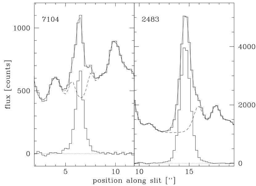
Figure 3: The spatial light distribution along two slitlets (left: star 7104, setup 1; right: star 2483, setup 2). The upper histogram is the observed light distribution, the grey continuous line gives the fit of all sources, the grey dashed line marks the subtracted sky background (= fit of all sources except target). The lower histogram is the spatial profile of the sky subtracted image.

Figure 4: Normalized spectra for all target stars. Spectral regions affected by cosmics are left out. On the right we show the region of the Mg 1b triplet, which is quite prominent in cool stars and may indicate contamination of our spectra by such stars.

Star 7567 shows a prominent G-band and a clear Mg 1b absorption, which in combination with its very red colour and high photometric error, suggest that this star has a cool companion (either a physical one or an unresolvable blend). It is therefore excluded from the further analysis and discussion.

4 Analysis

4.1 Atmospheric Parameters

For the analysis of the FORS2 spectra we used two sets of ATLAS9 model atmospheres (Kurucz kuru93 (1993)): For stars with $V<$ $\rm 17\stackrel{{\scriptstyle m}}{{.}}5$, which are presumably cooler than 11,000 K and therefore not affected by diffusion, we used a metallicity of [M/H] = $-0.5$ and solar helium abundance. For the fainter stars with $V>$ $\rm 18\stackrel{{\scriptstyle m}}{{.}}5$, which are presumably hotter than 12,000 K and therefore affected by diffusion, we used a super-solar metallicity of [M/H] = $+0.5$ and helium abundances ranging from solar to 1/100 solar. These models should account in a rough way for the effects of radiative levitation of heavy elements and gravitational settling of helium (see Moehler et al. mosw00 (2000) for details). From these model atmospheres we calculated spectra with Lemke’s version of the LINFOR program (developed originally by Holweger, Steffen, and Steenbock at Kiel University). To establish the best fit, we used the routines developed by Bergeron et al. (besa92 (1992)) and Saffer et al. (sabe94 (1994)), as modified by Napiwotzki et al. (nagr99 (1999)), which employ a $\chi^{2}$ test. The $\sigma$ necessary for the calculation of $\chi^{2}$ is estimated from the noise in the continuum regions of the spectra. The fit program normalizes model spectra and observed spectra using the same points for the continuum definition. We used the Balmer lines H_β to H₁₂ (excluding H_ϵ to avoid the Ca ii H line) for the fit. For the hot stars we included also the He i lines $\lambda\lambda$ 4026 Å, 4388 Å, 4471 Å, 4921 Å  to determine helium abundances, whereas the helium abundance was kept fixed at the solar value for the cool stars. The results are given in Table 3 and plotted in Fig. 5.

Recent tests have shown, however, that these fit routines underestimate the formal errors by at least a factor of 2 (Napiwotzki 2005, priv. comm.). In addition, the errors provided by the fit routine do not include possible systematic errors due to, e.g., flat field inaccuracies or imperfect sky subtraction. As we cannot estimate these systematic errors, we multiplied the formal errors by 2 to provide at least a lower limit to the errors.

4.2 Reddening

Using the effective temperatures derived this way, we also estimated reddenings by comparing the predicted colour from ATLAS9 model colours (for the same metallicities as the model spectra used in the fits) to the observed colours. Table 3 shows an obvious and very suspicious trend, namely, that the reddening increases towards higher effective temperatures: The cool stars show an average reddening of $\rm 0\stackrel{{\scriptstyle m}}{{.}}35$$\pm$$\rm 0\stackrel{{\scriptstyle m}}{{.}}05$, which is consistent with the literature value for NGC 6388. However, the fit results for stars below 9000 K are uncertain, as such stars show more and more metal lines, which are not included in the model spectra and possibly not evident in the observed spectra due to the low resolution of the data (although some lines can be seen in the spectra of the reddest stars 4113, 2483, and 1233 in Fig. 4). Restricting the averaging to the stars around 10,000 K yields a mean reddening of $\rm 0\stackrel{{\scriptstyle m}}{{.}}39$. The hot stars, however, show an average reddening of $\rm 0\stackrel{{\scriptstyle m}}{{.}}45$$\pm$$\rm 0\stackrel{{\scriptstyle m}}{{.}}04$, which is considerably larger than the accepted value. While Raimondo et al. (raca02 (2002)) report on possible differential reddening of up to $\rm 0\stackrel{{\scriptstyle m}}{{.}}1$, the correlation between reddening and temperature looks suspicious and might indicate an overestimate of the effective temperatures in the hot stars. As discussed below such an overestimate may be due to a partial filling of the line cores by residual light from cool stars (see Sect. 5.2).

Table 3: The atmospheric parameters and estimated reddenings from the spectroscopic analyses of our target stars. The spectroscopic results for stars below 9000 K (italized in table) are considered uncertain. For all stars below 11,000 K we assumed a solar atmospheric helium abundance, as these stars should not be affected by diffusion (see text for details).

star	${\rm T_{eff}}$	$\log{\rm g}$	${\rm\log{\frac{n_{He}}{n_{H}}}}$	${\rm E_{B-V}^{spec}}$
	[K]	[cm s-2]
396	10200$\pm$  300	3.52$\pm$0.12		$\rm 0\stackrel{{\scriptstyle m}}{{.}}360$
1233	7640$\pm$  110	2.85$\pm$0.12		$\it 0\stackrel{{\scriptstyle\rm m}}{{.}}287$
1283	17200$\pm$  760	4.28$\pm$0.12	$-$1.71$\pm$0.22	$\rm 0\stackrel{{\scriptstyle m}}{{.}}408$
1775	16100$\pm$  880	4.04$\pm$0.18	$-$1.68$\pm$0.32	$\rm 0\stackrel{{\scriptstyle m}}{{.}}464$
2483	7780$\pm$  110	2.97$\pm$0.12		$\it 0\stackrel{{\scriptstyle\rm m}}{{.}}345$
2612	24800$\pm$3300	4.68$\pm$0.38	$-$1.66$\pm$0.20	$\rm 0\stackrel{{\scriptstyle m}}{{.}}511$
2897	18700$\pm$1400	4.59$\pm$0.20	$-$1.48$\pm$0.32	$\rm 0\stackrel{{\scriptstyle m}}{{.}}451$
4113	7200$\pm$  140	2.72$\pm$0.22		$\it 0\stackrel{{\scriptstyle\rm m}}{{.}}323$
5235	9960$\pm$  320	3.61$\pm$0.16		$\rm 0\stackrel{{\scriptstyle m}}{{.}}385$
6239	19300$\pm$1900	4.33$\pm$0.26	$-$1.55$\pm$0.26	$\rm 0\stackrel{{\scriptstyle m}}{{.}}443$
7104	19500$\pm$2000	4.43$\pm$0.24	$-$2.06$\pm$0.36	$\rm 0\stackrel{{\scriptstyle m}}{{.}}429$
7788	10200$\pm$  280	3.51$\pm$0.14		$\rm 0\stackrel{{\scriptstyle m}}{{.}}360$

At least a part of the correlation might be due to the different effective temperatures of the stars. As discussed by Grebel & Roberts (grro95 (1995)) and others, the reddening effect of interstellar matter depends on the spectral type of a star. On average the reddening increases for bluer spectral types. Thus one would expect blue HB stars to have a higher reddening than the red giants in the same globular cluster. However, using their Fig. 9, we estimate that the reddening difference between red giants with [M/H] = $-0.5$ and blue tail stars with an atmospheric metallicity of [M/H] = $+0.5$ is at most about $\rm 0\stackrel{{\scriptstyle m}}{{.}}04$ for a reddening of ${\rm E_{B-V}}$ = $\rm 0\stackrel{{\scriptstyle m}}{{.}}37$ and the difference between cool blue HB stars and hot blue tail stars is below $\rm 0\stackrel{{\scriptstyle m}}{{.}}01$. This effect could therefore explain the slightly higher reddening of the cooler blue HB stars compared to the reddening of the cluster in general.

However, from the colour-magnitude diagram in Fig. 1, it is obvious that our “hot” targets have a higher reddening than the “cool” ones, as they lie all on the red side of the blue tail and in some cases even overlap with the cooler and brighter targets in $B-V$.

5 Comparison with Theoretical Tracks

Figure 5: Effective temperatures and surface gravities for our target stars as derived from line profile fits. For comparison we show the zero-age HB (ZAHB) for both a canonical helium abundance ($Y$ = 0.23, solid line) and two helium-rich compositions ($Y$ = 0.33, long dashed line; $Y$ = 0.43, short dashed line). For comparison we also show the results for the metal-poor globular cluster NGC 6752 from Moehler et al. (mosw00 (2000)).

We next compare the derived atmospheric parameters given in Table 3 with the theoretical HB tracks for both canonical and helium-rich compositions. Our goals are to determine if the blue tail stars provide any support for the helium enhancement predicted by the helium pollution scenario and, more specifically, to see if the stars near the top of the blue tail have the lower than canonical gravities inferred from the upward slope of the HB in NGC 6388. In Fig. 5 we plot the effective temperatures and surface gravities of our target stars together with the ZAHBs for a canonical helium abundance ($Y$ = 0.23) and two helium-rich compositions ($Y$ = 0.33, 0.43), as might arise from helium pollution. According to the helium pollution scenario, the helium abundance should increase along the HB from its canonical value in the reddest HB stars to a helium-rich value along the blue tail. Thus the blue tail stars should show the maximum offset from the canonical surface gravities.

The stars in Fig. 5 fall into three groups: three stars cooler than 9000 K, three stars near 10,000 K and six stars hotter than 12,000 K. As discussed in the previous section, the coolest stars with ${\rm T_{eff}}$ below 9000 K have less reliable parameters and thus will not be considered further.

5.1 Cool Blue Tail Stars Near 10,000 K

The moderately cool stars near 10,000 K lie above the canonical ZAHB in Fig. 5. At first glance this might be interpreted as evidence for a helium enhancement in these stars of perhaps as much as $Y$ $\approx$ 0.33. However, before drawing such a conclusion, we need to determine if the masses of these stars, as obtained from their atmospheric parameters, are consistent with the theoretical HB masses. Previous experience with the analysis of hot stars in globular clusters has shown that low surface gravities are often associated with impossibly small HB masses, thus indicating that the surface gravities are not reliable. To carry out this consistency check, we have estimated masses for all of our target stars using the approach outlined by Moehler et al. (mosw00 (2000)). Fig. 6 compares these masses with the theoretical ZAHB masses for both canonical and helium-rich compositions. We note that the ZAHB masses in Fig. 6 depend only weakly on the helium abundance. The mean mass of the cool blue tail stars is 0.52  $\rm M_{\odot}$ in good agreement with the theoretical masses.

Given this consistency check, we can now examine how the predicted surface gravity and luminosity of the cool blue tail stars depend on the helium abundance. In order to reduce the uncertainty in our results, we will use the average effective temperature and surface gravity of these stars instead of the individual measurements, i.e., $<$${\rm T_{eff}}$$>$ = 10,120 K and $<$log g$>$ = 3.547. These average values should better represent the mean atmospheric parameters during the HB phase. The dependence of the surface gravity at ${\rm T_{eff}}$ = 10,120 K on $Y$ is given in the top panel of Fig. 7 for stars at the ZAHB, at the midpoint of the HB phase and at the point 90% through the HB phase. We see that the bulk of the HB phase is spent within a narrow range in log g at a given helium abundance. Only near the end of the HB phase does the surface gravity decrease significantly below its ZAHB value. The corresponding variation in the luminosity with $Y$ is shown in the lower panel of Fig. 7. We again see that most of the HB phase is spent close to the ZAHB luminosity as long as $Y$ $\lesssim$ 0.35. At higher helium abundances an HB star will evolve along a blue loop that becomes increasingly more extended in effective temperature and that deviates more and more from the ZAHB. This leads to the substantial increase in the predicted luminosity width of the HB evident in Fig. 7.

The results in Fig. 7 are combined in Fig. 8 to show the predicted variation of the luminosity with surface gravity at ${\rm T_{eff}}$ = 10,120 K. The thin vertical line represents the mean surface gravity of our cool blue tail stars. We see that the luminosity at this surface gravity does not depend very much on whether the cool blue tail stars are near the ZAHB or near the end of the HB phase. Assuming that, on average, they are near the midpoint of the HB phase, we find a mean luminosity $<$log L$>$ of 1.62 for $\log{\rm g}$ = 3.547. The corresponding luminosity of a canonical HB star at the midpoint of its HB phase is log L = 1.46 at ${\rm T_{eff}}$ = 10,120 K. The difference in these luminosities implies that our cool blue tail stars are $\approx$0$\aas@@fstack{m}$4 brighter than canonical HB stars. This result is in reasonable agreement with the 0$\aas@@fstack{m}$5 increase in luminosity implied by the upward slope of the HB in NGC 6388. While our sample of cool blue tail stars is admittedly very small and the errors in their surface gravities significant, our results do suggest a brighter than canonical luminosity that is at least consistent with the scenarios that can explain the HB slope in NGC 6388.

One can also ask what helium abundance is required to produce the lower surface gravities of the cool blue tail stars. From the top panel of Fig. 7 we find that a mean surface gravity of log g = 3.547 corresponds to a helium abundance of $Y$ = 0.32 if the cool blue tail stars are in the main part of their HB phase. If, however, they are near the end of their HB phase, then the required helium abundance would be $Y$ = 0.28. In either case a helium enrichment, as might be expected from the helium pollution scenario, could account for the properties of the cool blue tail stars in our sample. Accounting for such an increased helium abundance in the theoretical model spectra, which were used to determine effective temperatures and surface gravities, would lower the derived surface gravities, because an increase in helium abundance broadens the Balmer line profiles. Thus a given observed profile will yield a lower surface gravity if fitted with helium-enriched model spectra.

Figure 6: Effective temperatures and masses for our target stars. For comparison we show both the canonical ZAHB ($Y$ = 0.23, solid line) and two helium-rich ZAHBs ($Y$ = 0.33, long dashed line; $Y$ = 0.43, short dashed line).

Figure 7: Predicted surface gravity and luminosity of HB stars at ${\rm T_{eff}}$ = 10,120 K as a function of the helium abundance $Y$. The solid curves refer to the ZAHB, the dashed curves to the midpoint of the HB phase, and the dotted curves to the point 90% through the HB phase.

Figure 8: Variation of the luminosity of HB stars at ${\rm T_{eff}}$ = 10,120 K with surface gravity over a range in the helium abundance from $Y$ = 0.23 to $Y$ = 0.43. The solid curve refers to the ZAHB, the dashed curve to the midpoint of the HB phase, and the dotted curve to the point 90% through the HB phase. The values of $Y$, indicated by the solid squares along the ZAHB curve, increase from $Y$ = 0.23 in the lower right to $Y$ = 0.43 in the upper left in increments of 0.05. The thin vertical line at log g = 3.547 denotes the mean gravity of the cool blue tail stars.

5.2 Blue Tail Stars Hotter Than 12,000 K

The hot blue tail stars in Fig. 5 have surface gravities that are substantially smaller than the canonical values and indeed even smaller than the surface gravities along the helium-rich ZAHB for $Y$ = 0.43. As in the case of the cool blue tail stars, we can use the masses obtained from the atmospheric parameters to test the reliability of these surface gravities. The masses of the hot blue tail stars plotted in Fig. 6 are, on average, about a factor of 2 smaller than the theoretically predicted masses and, moreover, are strongly correlated with the offset in log g from the ZAHB in Fig. 5. The only exception is star 2897 at ${\rm T_{eff}}$ = 18,700 K, which has a mass in good agreement with the theoretical value and which lies close to the $Y$ = 0.43 ZAHB in Fig. 5. The atmospheric parameters of star 2897, if representative of the true atmospheric parameters of a typical hot blue tail star, would be consistent with an increase in the helium abundance along the blue tail. However, the surface gravities of the other hot blue tail stars seem spuriously too low.

The fact that the cool blue tail stars, which are visually about 2 magnitudes brighter than the hot blue tail stars, have reasonable parameters in Figs. 5 and 6 suggests that the problems with the parameters of the hot blue tail stars may be due to problems with background subtraction. A possible effect would be a filling of the Balmer line cores by residual light from cool stars, which would simulate a higher effective temperature (= less deep cores) for the hotter stars. The wings would be less affected by such light, and the surface gravity determined from them would probably be closer to the true value. However, with our current data we have no way of verifying this possibility.

For comparison we show also results for stars in the metal-poor globular cluster NGC 6752, which were analysed in the same way as the stars discussed here, but are almost uncrowded. Obviously the stars in NGC 6388 show lower surface gravities at a given temperature than those in NGC 6752, whereas canonical stellar evolutionary theory would argue in the opposite direction. This may be taken as support for the influence of background subtraction. On the other hand, however, one should keep in mind that the helium enrichment required to produce hot HB stars in a metal-rich globular cluster would produce significantly higher luminosities and thus lower gravities.

Blue tail stars hotter than 12,000 K are also affected by radiative levitation which can increase the atmospheric metallicity to super-solar values (Behr et al. beco99 (1999), Moehler et al. mosw00 (2000), Moehler moeh01 (2001), Behr behr03 (2003)). We attempted to include this effect in our analysis by using metal-rich stellar atmospheres when determining the atmospheric parameters of the hot blue tail stars. However, these stellar atmospheres assume a scaled solar abundance distribution which may not adequately account for the highly non-solar abundance distribution produced by radiative levitation. Further study is needed to see if this difference between the assumed and actual abundance distributions can partly explain the low gravities of the hot blue tail stars. This explanation is supported by the low gravities found for hot blue tail stars in NGC 6752 (Moehler et al. mosw00 (2000)) and M 13 (Moehler et al. mola03 (2003)). It is important to note that the low helium abundances observed in the hot blue tail stars are caused by diffusion effects and do not contradict any helium pollution scenario.

Fig. 5 compares the surface gravities of the hot blue tail stars only with the surface gravities of ZAHB models. Since at high helium abundances the HB evolutionary tracks can deviate considerably from the ZAHB, we also need to examine how the post-ZAHB evolution affects the predicted gravities. In Fig. 9 we overplot the hot blue tail stars onto an HB simulation covering the entire HB phase for $Y$ = 0.43. For simplicity a uniform distribution in mass was assumed in this simulation. The hottest star in our sample (star 2612) is not included in Fig. 9 because its surface gravity is much too low to be explained by HB evolution. Not surprisingly, star 2897 lies within the bulk of the HB stars in Fig. 9. However, all of the other hot blue tail stars lie in regions that are poorly populated. We conclude that HB evolution is unlikely to account for the low surface gravities of the hot blue tail stars - a further indication of the uncertainty in the atmospheric parameters of these stars.

Figure 9: Comparison of the atmospheric parameters of the hot blue tail stars with an HB simulation for a helium abundance $Y$ = 0.43.

6 Conclusions

Our results for the cool blue tail stars in NGC 6388 are consistent with both the upward slope of the HB in NGC 6388 and the predictions of the helium pollution scenario. Moreover, they resolve the puzzling conundrum discussed by Moehler et al. (mosw99 (1999)), who found higher than canonical surface gravities for a sample of blue tail stars in NGC 6388 and NGC 6441 in contradiction to all scenarios for explaining the upward sloping HBs in these globular clusters. Most likely, these large gravities can be attributed to problems with the background subtraction from the spectra.

Our results for the hot blue tail stars remain problematical. The low surface gravities and masses found for these stars might be due to problems with the background subtraction or possibly to inadequacies in the stellar atmospheres used in the analysis. Further work is needed to clarify this point. Unfortunately the atmospheric parameters for the hot blue tail stars do not permit a stringent test of the helium pollution scenario. In particular, the present data cannot test the prediction for a greater gravity offset from the canonical ZAHB in the hot blue tail stars compared to the cool blue tail stars, as one would expect if the helium abundance increased along the blue tail.

The present study illustrates the difficulties encountered when doing spectroscopy in crowded fields. From our experience we conclude that the problem of the hot stars in NGC 6388 cannot be solved by means of current ground-based observations. One would need either optical spectra at a much better spatial resolution (around 0$\aas@@fstack{\prime\prime}$1) or multi-colour photometry including the near and far UV. Spectroscopy at such high spatial resolution is currently available only at near-IR wavelengths, which would worsen the contrast between the hot and cool stars and, in addition, would allow only the use of hydrogen lines, for which the model atmospheres have not been tested. Multi-colour photometry might provide an estimate of the effective temperatures and luminosities of these stars, but as they are hot, the satellite UV is definitely required.

- (1) Anderson, J. 1997, Ph.D. thesis, Univ. California, Berkeley
- (2) Behr, B. B. 2003, ApJS, 149, 67
- (3) Behr, B. B., Cohen, J. G., McCarthy, J. K. & Djorgovski, S. G. 1999, ApJ, 517, L135
- (4) Bekki, K. & Norris, J. E. 2006, ApJ, 637, L109
- (5) Bergeron, P., Saffer, R. A. & Liebert, J. 1992, ApJ, 394, 228
- (6) Cavallo, R. M., Sweigart, A. V. & Bell, R. A. 1998, ApJ, 492, 575
- (7) D’Antona, F., Bellazzini, M., Caloi, V., Fusi Pecci, F., Galleti, S. & Rood, R. T. 2005, ApJ, 631, 868
- (8) D’Antona, F. & Caloi, V. 2004, ApJ, 611, 871
- (9) Gratton, R. G., Bonifacio, P., Bragaglia, A., et al. 2001, A&A, 369, 87
- (10) Grebel, E. K. & Roberts, J. W. 1995, A&AS, 109, 293
- (11) Hamuy, M., Walker, A. R., Suntzeff, N. B., et al. 1992, PASP, 104, 533
- (12) Horne, K. 1986, PASP, 98, 609
- (13) Kraft, R. P. 1994, PASP, 106, 553
- (14) Kurucz, R. L. 1993, ATLAS9 Stellar Atmospheres Program and 2 km s-1 grid, CD-ROM No. 13, http://kurucz.harvard.edu/
- (15) Layden, A. C., Ritter, L. A., Welch, D. L., Webb, T. M. A. 1999, AJ, 117, 1313
- (16) Moehler, S. 2001, PASP, 113, 1162
- (17) Moehler, S. & Sweigart, A. V. 2006, Balt. Astron. 15, 41
- (18) Moehler, S., Sweigart, A. V. & Catelan, M. 1999, A&A, 351, 519
- (19) Moehler, S., Sweigart, A.V., Landsman, W.B. & Heber, U. 2000, A&A, 360, 120
- (20) Moehler, S., Landsman, W.B. Sweigart, A.V., & Grundahl, F. 2003, A&A, 405, 135
- (21) Napiwotzki, R., Green, P. J. & Saffer, R. A. 1999, ApJ, 517, 399
- (22) Norris, J. E. 2004, ApJ, 612, L25
- (23) Piotto, G., Sosin, C., King, I. R., et al., 1997, in Advances in Stellar Evolution, eds. R. T. Rood & A. Renzini, Cambridge University Press, Cambridge, 84
- (24) Piotto, G., Villanova, S., Bedin, L. R., et al. 2005, ApJ, 621, 777
- (25) Pritzl, B., Smith, H. A., Catelan, M. & Sweigart, A. V. 2000, ApJ, 530, L41
- (26) Pritzl, B., Smith, H. A., Catelan, M. & Sweigart, A. V. 2002, AJ, 124, 949
- (27) Pych, W. 2004, PASP, 116, 148
- (28) Raimondo, G., Castellani, V., Cassisi, S., Brocato, E. & Piotto, G. 2002, ApJ, 569, 975
- (29) Ree, C. H., Yoon, S.-J., Rey, S.-C. & Lee, Y.-W. 2002, in Centauri, A Unique Window into Astrophysics, eds. F. van Leeuwen, J. D. Hughes & G. Piotto, ASP Conf. Ser., 265, p.101
- (30) Rich, R. M., Sosin, C., Djorgovski, S. G., et al. 1997, ApJ, 484, L25
- (31) Saffer, R. A., Bergeron, P., Koester, D. & Liebert, J. 1994, ApJ, 432, 351
- (32) Sandage, A. & Wildey, R. 1967, ApJ, 150, 469
- (33) Sweigart, A. V. 2002, in Highlights of Astronomy, ed. H. Rickman, ASP, San Francisco, p. 292
- (34) Sweigart, A. V. & Catelan, M. 1998, ApJ, 501, L63 (SC98)
- (35) Tüg, H. 1977, ESOMe, 11, 7
- (36) van den Bergh, S. 1967, AJ, 72, 70