Braneworld inflation from an effective field theory after WMAP three-year data

Abstract

In light of the results from the WMAP three-year sky survey, we study an inflationary model based on a single-field polynomial potential, with up to quartic terms in the inflaton field. Our analysis is performed in the context of the Randall-Sundrum II braneworld theory, and we consider both the high-energy and low-energy (i.e. the standard cosmology case) limits of the theory. We examine the parameter space of the model, which leads to both large-field and small-field inflationary type solutions. We conclude that small-field inflation, for a potential with a negative mass square term, is in general favored by current bounds on the tensor-to-scalar perturbation ratio $r_{s}$.

I Introduction

Inflation, originally introduced to solve the initial condition problems of standard cosmology (SC) Guth (1981), is at present the favorite paradigm for explaining both the Cosmic Microwave Background Radiation (CMBR) temperature anisotropies and the initial conditions for structure formation. Indeed, it is during this epoch of accelerated expansion that the primordial density perturbations, which act as seeds for large-structure formation in the universe, are generated through the amplification of quantum fluctuations of the field(s) Mukhanov and Chibisov (1981). In the simplest inflationary models, the energy density of the universe is dominated by a single scalar field $\phi$, the so-called inflaton, that slowly rolls down its self-interaction potential.

The recent publication of the three year results of the Wilkinson Microwave Anisotropy Probe (WMAP) Hinshaw et al. (2006); Spergel et al. (2006) continues to support the standard inflationary predictions. WMAP data provides no indication of any significant deviations from gaussianity and adiabaticity of the CMBR power spectrum and suggests that the universe is spatially flat to within the limits of observational accuracy. Moreover, it allows for very accurate constraints on the spectral index; the WMAP three-year data (WMAP3) yield Spergel et al. (2006)

$$n_{s}=0.951^{+0.015}_{-0.019}~{},$$ (1)

at $68\%$ confidence level (CL), for vanishing running and no tensor modes. This result is in agreement with the one previously obtained in Ref. Sanchez et al. (2006), $n_{s}=0.954\pm 0.023$, using a joint analysis of the power spectrum of galaxy clustering measured from the final two-degree field galaxy redshift survey (2dfGRS) and a pre-WMAP3 compilation of measurements of both the temperature power spectrum and the temperature-polarization cross-correlation of the CMBR. A remarkable feature of these results is that the Harrison-Zel’dovich scale-invariant spectrum seems to be ruled out at around $3\sigma$ level.

Another feature of WMAP3 data is the evidence for a significant running of the scalar spectral index Spergel et al. (2006),

$$\alpha_{s}=-0.102^{+0.050}_{-0.043}~{},$$ (2)

at $68\%$ CL and considering tensor perturbations. This evidence was already present in the WMAP1 analysis Spergel et al. (2003) and persists when large scale structure data is included Spergel et al. (2006), although it is diluted by the addition of Lyman-$\alpha$ forest data Seljak et al. (2005); Lewis (2006); Seljak et al. (2006). We should note however that zero running is at about $2\sigma$ from the central value and hence WMAP3 does not demand a nonvanishing running. In fact, vanishing running is still a good fit to the CMBR data, and the improvement of the $\chi^{2}$ is small ($\Delta\chi^{2}=-3$), if running is allowed. Notice also that if both tensor modes and running are taken into account, the WMAP team obtained $n_{s}=1.21^{+0.13}_{-0.16}$ as the best fit value for the scalar tilt.

On the theoretical side, motivated by developments in string/M-theory, there has been considerable interest in the so-called braneworld constructions, where the matter fields are trapped in a lower dimensional brane, while (in the simplest models) only gravity can propagate into the bulk. Of special interest for cosmology is the Randall-Sundrum II (RSII) construction Randall and Sundrum (1999), consisting of a single brane with positive tension embedded in a 5-dimensional bulk with a negative cosmological constant (anti-de Sitter spacetime). A remarkable feature of the RSII brane cosmology (BC) is the modification of the expansion rate of the universe, $H=\dot{a}/a$, before the nucleosynthesis era Binetruy et al. (2000). While in standard cosmology the expansion rate scales with the energy density $\rho$ as $H\propto\sqrt{\rho}$, this dependence becomes $H\propto\rho$ at very high energies in brane cosmology. This behavior may have important consequences on early universe phenomena such as inflation Maartens et al. (2000); Bento and Bertolami (2002) and the generation of the baryon asymmetry Mazumdar (2001).

In this paper we study the RSII braneworld inflationary period in the light of WMAP3 results, for a single-field power-law inflaton potential of the form Hodges et al. (1990)

$$V(\phi)=V_{0}+\dfrac{1}{2}\,s\,m^{2}\,\phi^{2}+\dfrac{1}{3}\,m\,\widetilde{g}\,\phi^{3}+\dfrac{1}{4}\,\widetilde{\lambda}\,\phi^{4}~{}.$$ (3)

Here $s=1$ (unbroken symmetry) or $s=-1$ (broken symmetry) and $m>0$. The parameters $\widetilde{\lambda}$ and $\widetilde{g}$ are dimensionless constants; $\widetilde{\lambda}$ must be positive in order to ensure the stability of the potential, while $\widetilde{g}$ can have either sign.

This potential has been studied previously in the literature in the SC context Hodges et al. (1990); Cirigliano et al. (2005); Boyanovsky et al. (2006); de Vega and Sanchez (2006) and covers a wide class of inflationary scenarios: for both spontaneously broken and unbroken (negative and positive mass square term, respectively) potentials one can obtain small and large-field inflation (hereafter also called new and chaotic inflationary solutions, respectively). Monomial potentials have already been widely studied both in standard cosmology (for a recent update following WMAP3 data see Refs. Kinney et al. (2006); Alabidi:2006qa_plus ) and in the braneworld context Maartens et al. (2000); Bento and Bertolami (2002); Tsujikawa and Liddle (2004); these can be regarded as particular cases of the one considered here. It is also worth noticing that potentials of the type we are considering, Eq. (3), can be obtained as effective potentials in some supergravity models (for a recent study see Ref. Ibe et al. (2006)).

The paper is organized as follows. After discussing in Section II the main features of the inflaton potential, we briefly review in Section III the slow-roll inflation formalism in the braneworld context. In Section IV we present and discuss our results. Some final comments and conclusions are given in Section V.

Figure 1: The potential of Eq. (6) for the cases discussed in the text. The full (dashed) lines correspond to large (small) field inflation. The curves correspond to different values of the asymmetry parameter $h$: (a) $h=-0.2,0$, (b) $h=-0.8,0$ and (c) $h=-1.15,-\sqrt{9/8},-1.02$. We will only consider inflation occurring on the black branches of the potential (cf. Table 1).

	s	$h$ range	$\varphi$ range	Inflation type	Case
	$-1$	$h\leq 0$	$0\lesssim\varphi<\varphi_{+}$	Small-field (a)	A
	$-1$	$h\leq 0$	$\varphi>\varphi_{+}$	Large-field (a)	B
	$+1$	$-1\leq h\leq 0$	$\varphi>0$	Large-field (b)	C
	$+1$	$-\sqrt{9/8}\leq h\leq-1$	$0<\varphi\lesssim\varphi_{-}$	Large-field (c)	D
	$+1$	$h\leq-\sqrt{9/8}$	$\varphi_{-}\lesssim\varphi<\varphi_{+}$	Small-field (c)	E
	$+1$	$h\leq-\sqrt{9/8}$	$\varphi>\varphi_{+}$	Large-field (c)	F

Table 1: Cases A-F correspond to different ranges of the potential parameters and field values, see Eqs. (6) and (9), leading to large and small-field inflation. Labels (a)-(c) correspond to the cases shown in Fig. 1.

II Inflation from an effective field theory

The potential of Eq. (3) is the most general renormalizable (power law) potential. Of course, more complicated single-field potentials can be obtained from low-energy effective field theories, but the terms in the potential of Eq. (3) can, in many cases, be regarded as the leading terms in a power series expansion of such potentials, as e.g. it is the case of supergravity models. Moreover, as noticed in the Introduction, this single-field potential already covers different types of inflationary scenarios, namely small and large-field inflation.

In view of the stringent limits on the present vacuum energy density, a reasonable assumption is to set the global minimum of the potential to zero. This ensures that inflation does not run forever and ends with a finite number of e-folds. This also fixes the parameter $V_{0}$ in terms of the potential parameters $m$, $\widetilde{g}$ and $\widetilde{\lambda}$. One should also notice that the potential has a $\phi\rightarrow-\phi$, $\widetilde{g}\rightarrow-\widetilde{g}$ symmetry. Thus, in order to explore the parameter space it is sufficient to choose a definite sign for $\widetilde{g}$. In our analysis we will consider $\widetilde{g}\leq 0$ and assume $\phi$ to be positive.

In order to analyze the potential it is useful to redefine the inflaton field as

$$\varphi\equiv\dfrac{\phi}{M_{P}}~{},$$ (4)

where $M_{P}\simeq 2.4\times 10^{18}$ GeV is the reduced four-dimensional Planck mass, and rewrite the potential as

$$V(\varphi)=m^{2}\,M_{P}^{2}\;v(\varphi)~{},$$ (5)

where the dimensionless part is given by

$$v(\varphi)=v_{0}+\dfrac{1}{2}\,s\,\varphi^{2}+\dfrac{2}{3}\,g\,\varphi^{3}+\dfrac{1}{32}\,\lambda\,\varphi^{4}~{},$$ (6)

with

$$v_{0}=\dfrac{V_{0}}{m^{2}\,M_{P}^{2}}~{},~{}\quad g=\dfrac{\widetilde{g}\,M_{P}}{2\,m}~{},~{}\quad\lambda=\dfrac{8\,\widetilde{\lambda}\,M_{P}^{2}}{m^{2}}~{}.$$ (7)

The qualitative behavior of the potential is easily understood with the determination of the critical points (maxima, minima or inflection points), obtained from $v^{\prime}(\varphi)=0$, where the prime denotes the derivative with respect to the dimensionless field $\varphi$. There is a critical point at $\varphi_{0}=0$ and two more possible critical points (depending on the parameters $g$ and $\lambda$) at

$$\varphi_{\pm}=\dfrac{8\,|g|\pm 2\sqrt{16\,g^{2}-2\,s\,\lambda}}{\lambda}~{},$$ (8)

where we are restricting to the case $g\leq 0$.

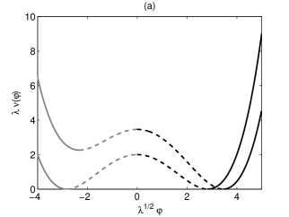
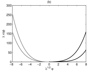
It is easy to see that for $s=-1$ the potential has one maximum at $\varphi_{0}=0$ and a global minimum at $\varphi_{+}$ (there is also a local minimum at $\varphi_{-}$, which for $g=0$ is degenerated with the first one) - see Fig. 1(a). The parameter $g$ determines the asymmetry of the potential: the larger its absolute value is, the more asymmetric is the potential. In this case, one can have both large and small-field inflation, depending on the initial value of the inflaton field (cases A and B in Table I).

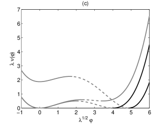
For $s=1$ we can distinguish two cases. If $\lambda\geq 8g^{2}$, the only critical point of the potential is $\varphi_{0}=0$, corresponding to the minimum of the potential. Once more, the larger $|g|$ is, the more asymmetric the potential becomes [see Fig. 1(b)]. In this case only large-field inflation is possible. If $\lambda<8g^{2}$, the potential has three critical points: one maximum at $\varphi_{-}$ and two minima at $\varphi_{0}$ and $\varphi_{+}$. For $\lambda=64\,g^{2}/9$ the minima are degenerated, for $\lambda>64\,g^{2}/9$ the global minimum is at $\varphi_{0}$ and for $\lambda<64\,g^{2}/9$ at $\varphi_{+}$ [see Fig. 1(c)]. In this parameter range we can have either small or large-field inflation.

It is useful to reformulate the previous discussion in terms of the parameter

$$h=g\,\sqrt{\dfrac{8}{\lambda}}~{}.$$ (9)

For $s=1$ and $-1\leq h\leq 0$ (we are considering only negative values of $g$), the potential has only one minimum at $\varphi_{0}=0$. In this case only large-field inflation is possible, corresponding to case C of Table 1. For $h<-\sqrt{9/8}$, the global minimum of the potential is at $\varphi_{+}$ (and there is a local minimum at $\varphi_{0}=0$). Both large and small-field inflation are possible but in order to obtain small-field inflation, case E of Table 1, the initial value of the field should lie between $\varphi_{-}$ and $\varphi_{+}$, thus implying a certain amount of fine-tuning; hence, we will consider only the large-field case. For the same reason, we will neglect the range $-\sqrt{9/8}<h<-1$, where the global minimum of the potential is at $\varphi_{0}=0$ and there is also a local minimum at $\varphi_{+}$, case D of Table 1. Notice also that, in Table 1, only the cases where the field rolls towards the global minimum are taken into consideration.

	$n_{s}^{high}$	$r_{s}^{high}$	$n_{s}^{low}$	$r_{s}^{low}$
$p$	$\dfrac{(p+2)\,N_{\star}-3\,p-2}{(p+2)\,N_{\star}+p}$	$\dfrac{24\,p}{(p+2)\,N_{\star}+p}$	$\dfrac{2\,N_{\star}-3}{2\,N_{\star}-1+p}$	$\dfrac{8\,p}{2\,N_{\star}-1+p}$
$2$	$\dfrac{2\,(N_{\star}-2)}{2\,N_{\star}+1}=0.959$	$\dfrac{24}{2\,N_{\star}+1}=0.20$	$\dfrac{2\,N_{\star}-3}{2\,N_{\star}+1}=0.967$	$\dfrac{16}{2\,N_{\star}+1}=0.13$
$4$	$\dfrac{3\,N_{\star}-7}{3\,N_{\star}+2}=0.951$	$\dfrac{48}{3\,N_{\star}+2}=0.26$	$\dfrac{2\,N_{\star}-3}{2\,N_{\star}+3}=0.951$	$\dfrac{32}{2\,N_{\star}+3}=0.26$

Table 2: High- and low-energy limits in the RS II braneworld model for the scalar spectral index $n_{s}$ and the tensor-to-scalar perturbation ratio $r_{s}$, in the case of a simple monomial inflationary potential of the form $V\propto\phi^{p}$. The numerical values are computed taking $N_{\star}=60$.

III Slow-roll braneworld inflation

We will consider the RSII scenario, where all matter fields are confined to the brane and, hence, inflation is driven by a 4D scalar field trapped on the brane. In this scenario, the detailed form of perturbations produced by the inflationary potential is modified due to the modification of the Friedmann equation at high energies and because gravitational wave perturbations are able to go into the bulk. In fact, in a cosmological scenario in which the metric projected onto the brane is a spatially flat Friedmann-Lemaître-Robertson-Walker model, the Friedmann equation in 4D acquires an extra term, becoming Binetruy et al. (2000)

$$H^{2}={1\over 3\,M_{P}^{2}}\,\rho\,\left[1+{\rho\over 2\widetilde{\sigma}}\right]~{},$$ (10)

after setting the four-dimensional cosmological constant to zero and assuming that inflation rapidly makes any dark radiation term negligible. The brane tension $\widetilde{\sigma}$ relates the four- and five-dimensional Planck masses through the relation

$$\widetilde{\sigma}=\frac{3}{32\pi^{2}}\frac{M_{5}^{6}}{M_{P}^{2}}~{},$$ (11)

where $M_{5}$ is the 5D Planck mass. Notice that Eq. (10) reduces to the usual Friedmann equation at sufficiently low energies, $\rho\ll\widetilde{\sigma}$, while at very high energies we have $H\propto\rho$. Successful big bang nucleosynthesis (BBN) requires that the change in the expansion rate due to the new terms in the Friedmann equation be sufficiently small at scales $\sim\mathcal{O}$(MeV); this implies $M_{5}\gtrsim 40~{}\mbox{TeV}$ Cline et al. (1999). A more stringent bound, $M_{5}\gtrsim 10^{5}~{}\mbox{TeV}$, is obtained by requiring the theory to reduce to Newtonian gravity on scales larger than 1 mm Maartens et al. (2000). For the sake of convenience, in the following we shall work with a dimensionless brane tension defined as

$${\sigma}=\frac{\widetilde{\sigma}}{m^{2}\,M_{P}^{2}}~{}.$$ (12)

Since the scalar field is confined to the brane, the conservation equation implies that the field satisfies the usual Klein-Gordon equation,

$$\ddot{\varphi}+3\,H\,\dot{\varphi}+m^{2}\,v^{\prime}(\varphi)=0~{},$$ (13)

where $v(\varphi)$ is the dimensionless potential defined in Eq. (6), and the prime denotes the derivative with respect to the dimensionless field $\varphi$. The high-energy corrections provide increased Hubble damping,

$$H^{2}\simeq{m^{2}\over 3}\,v\,\left[1+{v\over 2\,\sigma}\right]~{},$$ (14)

which makes the evolution of the inflaton slower.

Figure 2: $n_{s}$ as a function of $\widetilde{\lambda}$ and $M_{5}$ (upper panel) and $r_{s}$ as a function of $\widetilde{\lambda}$ and $M_{5}$ (lower panel), in the RSII braneworld model, for the potential of Eq. (3), broken symmetry case. Gray (black) lines indicate small (large) field inflationary solutions (respectively, cases A and B of Table I). The numbers $10^{-4}-10^{2}$ refer the value of the brane tension $\sigma$. The asymmetry parameter h is fixed at $|h|=1$ and we have taken $N_{\star}=60$. The horizontal dashed lines indicate the observational bounds on $n_{s}$ and the dot-dashed lines correspond to the upper bound on $r_{s}$, see Eqs. (32) and (33).

Figure 3: As in Fig. 2, but for the case of unbroken symmetry and large-field inflation (case C of Table I). We take $|h|=0.1$.

The number of e-folds during the inflationary period is given in the slow-roll approximation by Maartens et al. (2000)

$$N(\varphi)\simeq-\int_{\varphi}^{\varphi_{\rm F}}\dfrac{v}{v^{\prime}}\left[1+{v\over 2\,\sigma}\right]d{\varphi}~{},$$ (15)

where the subscript F corresponds to the end of inflation. Braneworld effects at high energies increase the Hubble rate by a factor $v/2\,\sigma$, yielding more inflation between any two values of $\varphi$ for a given potential. The value of $\varphi$ at the end of inflation can be obtained from the condition

$${\rm max}\{\epsilon(\varphi_{F}),|\eta(\varphi_{F})|\}=1~{},$$ (16)

where the slow-roll parameters are now defined as

$$\epsilon ={1\over 2}\left({v^{\prime}\over v}\right)^{2}{1+{v/\sigma}\over(1+{v/2\,\sigma})^{2}}~{},$$ (17)

$$\eta ={v^{\prime\prime}\over v}{1\over 1+{v/2\,\sigma}}~{}.$$ (18)

The prediction for the inflationary variables typically depends on the number of e-folds of inflation occurring after the observable universe leaves the horizon, $N_{\star}=N(\varphi_{\star})$. Although a wide variety of assumptions about $N_{\star}$ can be found in the literature, the determination of this quantity requires a model of the entire history of the universe. However, while from nucleosynthesis onwards this is now well established, at earlier epochs there are considerable uncertainties such as the mechanism ending inflation and details of the reheating process. This issue has been recently reviewed in Refs. Liddle and Leach (2003); Dodelson and Hui (2003), where a model-independent upper bound was derived, namely $N_{\star}<60$. In fact, $N_{\star}=55$ is found to be a reasonable fiducial value with an uncertainty of about 5 e-folds around that value. However, the authors stress that there are several ways in which $N_{\star}$ could lie outside that range, in either direction. Moreover, in the braneworld context, one expects $N_{\star}$ to depend on the brane tension. Actually, larger values of $N_{\star}$ are expected because, in the high-energy regime, the expansion laws corresponding to matter and radiation domination are slower than in the standard cosmology, which implies a greater change in $aH$ relative to the change in $a$, therefore requiring a larger value of $N_{\star}\,$. This was confirmed by the results of Ref. Wang and Abdalla (2004), where the bound $N_{\star}<75$ was found for brane-inspired cosmology. In what follows we shall use $N_{\star}=60$.

In the RSII model, the scalar and tensor perturbation amplitudes are given by Maartens et al. (2000); Langlois et al. (2000)

$$A_{s}^{2} =\dfrac{m^{2}}{75\,\pi^{2}\,M_{P}^{2}}\,\dfrac{v^{3}}{v^{\prime 2}}\left[1+\dfrac{v}{2\,\sigma}\right]^{3}~{},$$ (19)

$$A_{t}^{2} =\dfrac{m^{2}}{150\,\pi^{2}\,M_{P}^{2}}\,v\,\left(1+\dfrac{v}{2\,\sigma}\right)F^{2}~{},$$ (20)

where

$$F^{2}=\left[\sqrt{1+x^{2}}-x^{2}\sinh^{-1}\left({1\over x}\right)\right]^{-1}~{},$$ (21)

and

$$x\equiv\left(\dfrac{3\,H^{2}}{4\pi\,m^{2}\,\sigma}\right)^{1/2}=\left[\dfrac{2\,v}{\sigma}\left(1+\dfrac{v}{2\,\sigma}\right)\right]^{1/2}~{}.$$ (22)

In the low-energy limit ($x\ll 1$), $F^{2}\approx 1$, whereas $F^{2}\approx 3\,v/2\,\sigma$ in the high-energy limit. The right hand side of Eqs. (19) and  (20) should be evaluated at horizon crossing, $k=aH$, where $k$ is the commoving wavenumber, which in terms of the inflaton field, corresponds to setting $\varphi=\varphi_{\star}$.

The mass parameter $m$ can be determined from Eq. (19),

$$m=5\sqrt{3}\,\pi\,M_{P}\,\dfrac{v^{\prime}}{v^{3/2}}\left[1+\dfrac{v}{2\,\sigma}\right]^{-3/2}A_{s}^{cmb}~{},$$ (23)

where $A_{s}^{cmb}$ is given by the WMAP amplitude of density fluctuations $A_{s}^{2}\approx 4.72\times 10^{-10}A$ with $A(k=0.002~{}{\rm Mpc}^{-1})\sim 0.8$. Notice that while in SC the mass parameter $m$ is fixed by the other potential parameters, in BC there is an extra degree of freedom - the brane tension.

The tensor power spectrum can be parameterized in terms of the tensor-to-scalar ratio as

$$r_{s}\equiv 16\,\dfrac{A_{t}^{2}}{A_{s}^{2}}~{},$$ (24)

where we have chosen the normalization so as to be consistent with the one of Refs. Peiris et al. (2003); Spergel et al. (2006), in the low-energy limit. WMAP3 Spergel et al. (2006) alone gives $r_{s}<0.55$ (with vanishing running) and $r_{s}<1.5$ (with running), both at $95\%$ CL. However, models with higher values of $r_{s}$ require larger values of $n_{s}$ and lower amplitude of the scalar fluctuations in order to fit the CMBR data, and these are in conflict with large scale structure measurements (in the case of vanishing running). Hence the strongest overall constraints on the tensor mode contribution comes from the combination of CMBR and large scale structure data. The combination of WMAP3 and Sloan Digital Sky Survey (SDSS) measurements Spergel et al. (2006) give: $r_{s}<0.28$ (without running) and $r_{s}<0.67$ (with running), at $95\%$ CL. If the Lyman-$\alpha$ forest spectrum from SDSS is also considered, then Seljak et al. (2006) $r_{s}<0.22$ (at $95\%$ CL and without running).

The spectral tilt for scalar perturbations can be written in terms of the slow-roll parameters as  Maartens et al. (2000)

$$n_{s}-1 \equiv{d\ln A_{s}^{2}\over d\ln k}=-6\,\epsilon+2\,\eta~{}.$$ (25)

The tensor index

$$n_{t} \equiv{d\ln A_{t}^{2}\over d\ln k}$$ (26)

obeys a more complicated equation Huey and Lidsey (2001). However, it can be shown that the consistency relation

$$n_{t}=-\dfrac{r_{s}}{8}$$ (27)

holds independent of the brane tension and, consequently, it has precisely the same form as the one obtained in standard cosmology. This means that perturbations do not contain any extra information as compared to SC, and, in particular, that they cannot be used to determine the brane tension: for any value of $\sigma$ one can always find a potential that generates the observed spectra Liddle and Taylor (2002).

The running of the scalar spectral tilt

$$\alpha_{s}\equiv{dn_{s}\over d\ln k}$$ (28)

can also be written in terms of the slow-roll parameters for the two limiting cases

$$\alpha_{s} =16\,\epsilon\,\eta-24\,\epsilon^{2}-2\,\xi\quad\quad{\rm for}~{}~{}v/\sigma\ll 1~{}~{}{\rm(SC)}~{},$$ (29)

$$\alpha_{s} =16\,\epsilon\,\eta-18\,\epsilon^{2}-2\,\xi\quad\quad{\rm for}~{}~{}v/\sigma\gg 1~{}~{}{\rm(BC)}~{},$$ (30)

where

$$\xi=\dfrac{v^{\prime}\,v^{\prime\prime\prime}}{v^{2}}\dfrac{1}{\left(1+{v/2\,\sigma}\right)^{2}}~{}$$ (31)

is the “jerk” parameter.

Figure 4: $n_{s}$ as a function of $\widetilde{\lambda}$ and $m$ (upper panel) and $r_{s}$ as a function of $\widetilde{\lambda}$ and $n_{s}$ (lower panel), in the SC limit, for the potential of Eq. (3), broken symmetry case. Gray (black) lines indicate small (large) field inflationary solutions (cases A and B of Table I, respectively). The numbers $0.1-100$ refer to the value of $|h|$ for each curve and $N_{\star}=60$ is assumed. Horizontal dashed lines indicate the observational bounds on $n_{s}$ and the dot-dashed lines correspond to the upper bound on $r_{s}$, see Eqs. (32) and (33).

Figure 5: As for Fig. 4 but for the case of unbroken symmetry, large-field inflation (black and gray lines correspond to cases C and F of Table I, respectively).

In the following we will analyze the different regimes (broken/unbroken, small/large field) for the potential of Eq. (5), in the braneworld context, taking into account the bounds obtained from the WMAP3 data. For completeness we will also study the low-energy limit ($v/\sigma\ll 1$), i.e. the standard cosmology limit. It is also interesting to consider the limiting cases of the monomial potentials $V\propto\phi^{p}$, for $p=2$ or $4$, obtained, for $s=1$, when $\lambda\rightarrow 0$ and $\lambda\gg 1$, respectively. In these cases the inflationary observables depend only on the number of e-folds of inflation occurring after the observable universe leaves the horizon, $N_{\star}$. In Table 2 we show the values of the scalar spectral index and ratio of tensor-to-scalar perturbations, as a function of $N_{\star}$, for monomial potentials of the form $V\propto\phi^{p}$, both in the high- and low-energy limits of brane cosmology.

We also remark in the models under consideration, the running $\alpha_{s}\sim 10^{-4}$ is very small, and therefore, one can make use of the observational bounds obtained in the case of vanishing running. If besides the WMAP3 data we also take into account the galaxy clustering and supernovae data, as well as the Lyman-$\alpha$ forest power spectrum data from SDSS, these bounds are Seljak et al. (2006)

$$n_{s} =0.965\pm 0.012~{}\left(\,{}^{+0.025}_{-0.024}\,\right)~{},$$ (32)

$$r_{s} <0.22~{}\left(\,<0.37\,\right)~{}.$$ (33)

The error bars are at $1\sigma$ ($2\sigma$) and the upper bounds at $95\%$ ($99.9\%$) CL. The recent analysis of Kinney et al Kinney et al. (2006) is in good agreement with Refs. Lewis (2006); Seljak et al. (2006), but shows significant inconsistencies with the results of WMAP3 team Spergel et al. (2006). Moreover, in their analysis the Harrison-Zel’dovich scale-invariant spectrum, with no running and no tensor component, is consistent with the WMAP3 data alone at 95$\%$ CL. In our numerical analysis and the discussion that follows we shall use the bounds given in Eqs. (32) and (33).

IV Results and discussion

In this Section we present the predictions for the density fluctuations in the RSII braneworld context for the case of the inflationary potential given by Eq. (3).

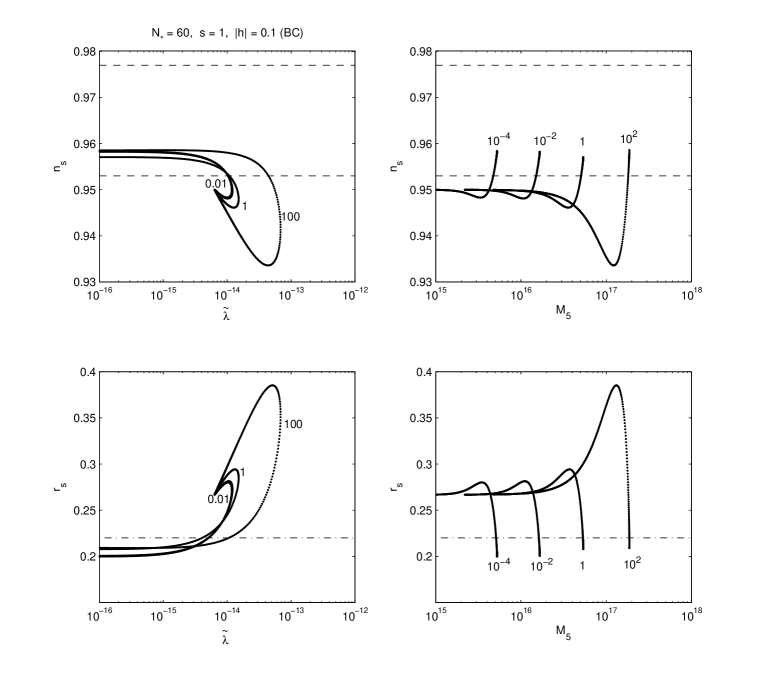
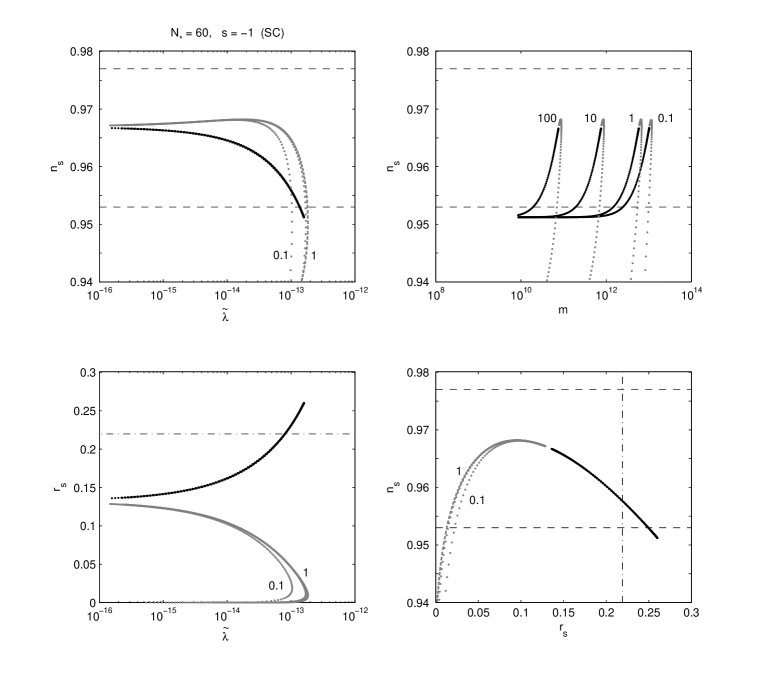
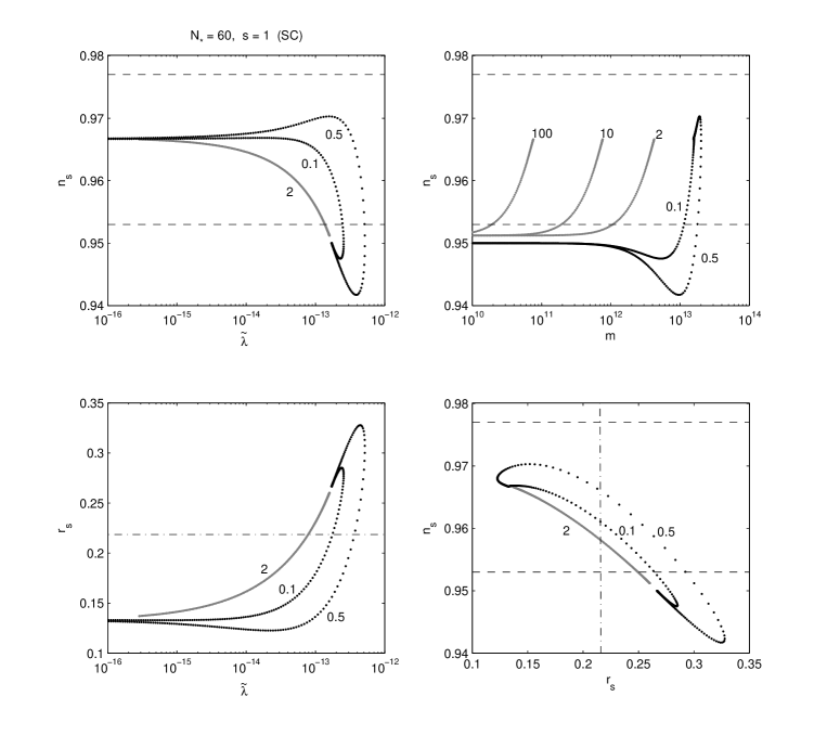
In Fig. 2 we plot $n_{s}$ as a function of $\widetilde{\lambda}$ and $M_{5}$ (upper panel) and $r_{s}$ as a function of $\widetilde{\lambda}$ and $M_{5}$ (lower panel) for the broken symmetry case ($s=-1$). Gray (black) lines indicate small (large) field inflationary solutions, which correspond to cases A and B of Table I, respectively. For illustration, the asymmetry parameter $|h|$ is fixed at $|h|=1$. The numbers $0.1-100$ refer to the value of the brane tension $\sigma$ for each curve, and $N_{\star}=60$ is assumed. Horizontal dashed lines indicate (upper and lower) observational bounds on $n_{s}$ and dot-dashed lines the upper bound on $r_{s}$ as given in Eqs. (32) and (33).

We see from Fig. 2 that, in the broken symmetry case, the new inflationary solutions are favored as compared with chaotic ones when we take into consideration the observational bound on $r_{s}$. In fact, chaotic inflationary solutions for a quartic polynomial potential, yield larger values of $r_{s}$ than the new inflationary ones for a given value of $n_{s}$. This feature is also present in standard cosmology, as first pointed out in Ref. Cirigliano et al. (2005). For comparison, the SC case is presented in Fig. 4, where we show $n_{s}$ as a function of the quartic coupling $\widetilde{\lambda}$ and the mass parameter $m$ (upper panel) and $r_{s}$ as a function of $\widetilde{\lambda}$ and $n_{s}$ (lower panel), for different values of $|h|$. Notice also that the fact that new inflation is favored over chaotic inflation is even more evident in the high-energy regime of BC than in the SC limit. This is already apparent from Table II, for the limiting case of the $\varphi^{2}$ potential, since we need higher values of $N_{\star}$ to satisfy the $r_{s}$ bound in BC ($N_{\star}>54$) than in SC ($N_{\star}>36$). As expected, in order to reproduce the CMB density fluctuations, the value of the quartic coupling $\widetilde{\lambda}$ should be small; we get the bound $\widetilde{\lambda}\lesssim 10^{-13}$.

In Fig. 3 we show the results for the case of unbroken symmetry, choosing $|h|=0.1$, which corresponds to case C of Table I (case F leads to results that are similar to case B, see Fig. 2). Remarkably, this type of solutions will be excluded for $r_{s}<0.2$, noticeably close to the bound given in Eq. (33). Comparing with the corresponding case in SC (cf. Fig. 5), we see that the high-energy regime of BC is indeed much more constrained by the $r_{s}$ bound. In this case, we get the upper bound $\widetilde{\lambda}\lesssim 10^{-12}$. This bound, together with the relation $|\widetilde{g}|=2\,|h|\,\widetilde{\lambda}^{1/2}$ and the condition $|h|\leq 1$, leads then to the following bound on the cubic coupling: $|\widetilde{g}|\lesssim 10^{-6}$.

Let us now briefly comment on the inflaton mass scale $m$, which is fixed by the amplitude of the scalar adiabatic fluctuations, as can be readily seen from Eq. (23). In the SC case and for small values of $|h|$, using the e-fold equation (15) one expects $\varphi\sim\mathcal{O}(\sqrt{N}),\,v(\varphi)\sim\mathcal{O}(N)$ and $v^{\prime}(\varphi)\sim\mathcal{O}(\sqrt{N})$ at horizon exit. Thus, we obtain

$$m\simeq 5\sqrt{3}\,\pi\,M_{P}\,\frac{A_{s}^{cmb}}{N_{\star}}\simeq 2\times 10^{13}~{}\textrm{GeV}.$$ (34)

On the other hand, for large values of $|h|$, one can show that there is an additional suppression factor $\mathcal{O}(1/|h|)$. In this case, higher values of the asymmetry parameter $|h|$ would require smaller values of the inflaton mass $m$ in order to correctly reproduce $A_{s}^{cmb}$. Such a behavior is also evident from Figs. 4 and Fig. 5.

In the high-energy BC regime, Eq. (15) suggests the scaling behavior $\varphi\sim\mathcal{O}[(\sigma N)^{1/4}],\,v(\varphi)\sim\mathcal{O}[(\sigma N)^{1/2}]$ and $v^{\prime}(\varphi)\sim\mathcal{O}[(\sigma N)^{1/4}]$ at horizon exit. Therefore, from Eqs. (11), (12) and (23) one finds for $|h|\lesssim 1$,

$$m\simeq\frac{(5\sqrt{\pi}\,A_{s}^{cmb})^{2/3}}{N_{\star}^{5/6}}\,M_{5}\simeq 10^{-4}\,M_{5}\,.$$ (35)

Moreover, as in the SC case, large values of $|h|$ imply smaller values of $m$ due to an extra suppression $\mathcal{O}(1/|h|)$.

After inflation ceases, the inflaton field starts to oscillate near the minimum of the effective potential, gradually producing a large number of particles, which interact with each other and come to a state of thermal equilibrium at some temperature $T_{\textrm{reh}}$, the reheating temperature. While we do not wish to commit ourselves to any specific reheating model, thus keeping our discussion as general as possible, we can make a rough estimate of the reheating temperature using the relation between $N_{\star}=N(k_{\star})$, the number of e-folds before the end of inflation when the scale of wavenumber $k_{\star}$ crosses the Hubble radius during inflation, i.e. when $k=aH$, and the energy density at the end of the reheating period, $\rho_{\textrm{reh}}$. Although such a relation crucially depends on the entire history of the universe, a plausible estimate can be obtained under simple assumptions about the sequence of epochs which follow inflation. We also recall that in the high-energy regime of brane cosmology the expansion laws during the matter and radiation dominated eras are slower than in standard cosmology. Nevertheless, the behavior of the densities is unchanged with respect to the scale factor.

Using the slow-roll approximation during inflation one can write Liddle and Leach (2003)

$$N_{\star}= \,\ln\dfrac{k_{\star}^{-1}}{3000\,h^{-1}\mbox{Mpc}}+\dfrac{1}{12}\ln\dfrac{\rho_{\textrm{reh}}}{\rho_{\textrm{end}}}+\dfrac{1}{4}\ln\dfrac{\rho_{\textrm{eq}}}{\rho_{\textrm{end}}}$$

$$+\ln\dfrac{H_{\star}}{H_{\textrm{eq}}}+\ln 219\,\Omega_{m}\,h\,,$$ (36)

where $H_{\textrm{eq}}$ and $H_{\star}=H(k_{\star})$ are the values of the Hubble radius at the matter-radiation equality epoch and at the scale $k_{\star}$, respectively; $\rho_{\textrm{end}}$ and $\rho_{\textrm{eq}}$ are the values of the energy density at the end of inflation and at equilibrium; $\Omega_{m}$ is the fractional matter energy density at present. We have

$$H_{\textrm{eq}} =5.25\times 10^{6}h^{3}\,\Omega_{m}^{2}\,H_{0}~{},$$ (37)

$$H_{0} =8.77\times 10^{-61}h\,M_{P}~{},$$ (38)

$$\rho_{\textrm{reh}} =\dfrac{\pi^{2}}{30}\,g_{*}\,T_{\textrm{reh}}^{4}\,,$$ (39)

where $H_{0}$ is the present Hubble radius and $g_{*}\simeq\mathcal{O}(10^{2})$ is the effective number of relativistic degrees of freedom. The CMBR anisotropy measured by WMAP allows a determination of the fluctuation amplitude at the scale $k=0.002~{}\mbox{Mpc}^{-1}$ and we use the WMAP3 central values $h=0.73,~{}\Omega_{m}h^{2}=0.127$ Spergel et al. (2006).

We find that, for an inflationary period driven by the power-law potential of Eq. (3), the relation

$$T_{\textrm{reh}}^{SC}\simeq(10^{7}-10^{8})\times e^{3(N_{\star}-55)}~{}\mbox{GeV}~{},$$ (40)

provides a good fit to our numerical results in the SC limit, as we allow $N_{\star}$ to vary in the expected range $55\leq N_{\star}\leq 70$ (see discussion in Section III). Similarly, in the high-energy regime of BC we get

$$T_{\textrm{reh}}^{BC}\sim 10^{2}\,\dfrac{M_{5}}{M_{P}}\,T_{\textrm{reh}}^{SC}~{},$$ (41)

which is valid for $M_{5}\lesssim 10^{-2}M_{P}\approx 10^{16}$ GeV. For larger values of $M_{5}$, $M_{5}>10^{16}$ GeV, one has $T_{\textrm{reh}}^{BC}\simeq T_{\textrm{reh}}^{SC}$. We also remark that the variation of $T_{\textrm{reh}}$ as a function of the density fluctuation parameters $n_{s}$ and $r_{s}$ is mild in both the SC and BC regimes.

V Conclusions

In this paper we have explored inflationary solutions for a single-field polynomial potential, with up to quartic terms in the inflaton field, in light of the results from the WMAP three-year sky survey. Our analysis is done in the framework of the Randall-Sundrum II braneworld theory, and we have examined both the high-energy and standard cosmology regimes. As in the case of SC, the model displays large-field and small-field inflationary type solutions compatible with the observational data.

For a potential with a negative mass square term, cases A and B of Table I, we conclude that small-field inflation is in general favored by current bounds on $r_{s}$. We also get the bound $\widetilde{\lambda}\lesssim 10^{-13}$ on the quartic coupling of the inflaton potential. The case with positive mass square term and $|h|\leq 1$ (large-field solutions), which corresponds to case C of Table I, is also very much constrained by the $r_{s}$ bound and, in particular, this type of solutions will be excluded if, as expected, $r_{s}<0.2$. In this case we get the following bounds on the parameters of the inflationary potential: $\widetilde{\lambda}\lesssim 10^{-12}$ and $|\widetilde{g}|\lesssim 10^{-6}$.

We have also made an estimate of the reheating temperature for this model and we have found that, for $M_{5}>10^{16}$ GeV and $N_{\star}\leq 60$, one has $T_{\textrm{reh}}^{BC}\simeq T_{\textrm{reh}}^{SC}\lesssim 10^{13}-10^{14}$ GeV, whereas for $M_{5}<10^{16}$ GeV, one gets the relation $T_{\textrm{reh}}^{BC}\sim 10^{2}\,T_{\textrm{reh}}^{SC}{M_{5}}/{M_{P}}\,$. At this point, it is worth noting that in supergravity models the presence of the gravitino could lead to serious cosmological problems unless the reheating temperature is sufficiently low. In particular, in gravity-mediated supersymmetry breaking models, the gravitino mass is expected in the range $m_{3/2}\sim\mathcal{O}(10^{2-4})$ GeV. Such a gravitino is most likely unstable and its decays could destroy the light elements synthesized during BBN. On the other hand, in gauge-mediated supersymmetry breaking models, the gravitino can be the lightest supersymmetric particle, and thus stable, with a mass $m_{3/2}\lesssim\mathcal{O}(10)$ GeV. In this case, its contribution to the present cosmic density can be excessive. In either case, this leads to stringent constraints on $T_{\textrm{reh}}$ after inflation Kawasaki et al. (2006). In the braneworld scenario, one expects such bounds to translate into additional constraints on the 5D fundamental Planck mass $M_{5}$.

Finally, let us comment on the running of the scalar index $\alpha_{s}$. One should notice that it is not possible to obtain large values for $\alpha_{s}$, either in SC or the high-energy BC scenarios, for polynomial potentials of the form given in Eq. (3). However, this is still consistent with observation, since the evidence for running is still weak and it can evaporate as more data becomes available. In fact, the addition of Lyman-$\alpha$ forest data reduces the need for a negative value of $\alpha_{s}$ Seljak et al. (2005); Lewis (2006); Seljak et al. (2006). Recently Easther $\&$ Peiris Easther:2006tv have analyzed the implications of a large running spectral index for single-field slow-roll inflation in SC, using the inflationary flow equations Hoffman:2000ue_plus ; Liddle:2003py and retaining all terms in $\alpha_{s}$ up to quadratic order in the slow-roll parameters. They found that, for all parameter choices consistent with a large negative running, inflation lasts less than 30 e-folds after CMBR scales leave the horizon. They concluded that a definitive observation of a large negative running would imply that inflationary stage requires multiple fields or the breakdown of slow-roll. The underlying conclusions of their work can presumably be carried over to the BC case, as the flow equations are quite insensitive to the expansion dynamics Ramirez:2004fb . However, one should notice, as shown in Liddle:2003py , that the flow equation approach does not directly incorporate inflationary dynamics. In fact, one can determine analytically the set of inflationary potentials which correspond to solutions of the truncated flow equations. Hence, conclusions obtained from an analysis based on the flow equations should be considered with some care, since it is certainly possible to find potential shapes that are not represented by the set of inflationary potentials for which the formalism is valid. An example of a model where it is possible to obtain a considerably large running was explored in Ref. Ballesteros:2005eg .