Submillimeter Wave Astronomy Satellite observations of comet 9P/Tempel 1
and Deep Impact

, , , , , ,

Proposed Running Head:
SWAS observations of 9P/Tempel 1

Please send Editorial Correspondence to:
Frank Bensch
Argelander Institut für Astronomie
Abteilung Radioastronomie
Auf dem Hügel 71
53121 Bonn, Germany.

Email: fbensch@astro.uni-bonn.de
Phone: +49 (228) 73-1774
Fax: +49 (228) 72-1775

ABSTRACT

On 4 July 2005 at 5:52 UT the Deep Impact mission successfully completed its goal to hit the nucleus of 9P/Tempel 1 with an impactor, forming a crater on the nucleus and ejecting material into the coma of the comet. NASA’s Submillimeter Wave Astronomy Satellite (SWAS) observed the $1_{10}-1_{01}$ ortho-water ground-state rotational transition in comet 9P/Tempel 1 before, during, and after the impact. No excess emission from the impact was detected by SWAS and we derive an upper limit of $1.8\times 10^{7}$ kg on the water ice evaporated by the impact. However, the water production rate of the comet showed large natural variations of more than a factor of three during the weeks before and after the impact. Episodes of increased activity with $Q_{\rm H_{2}O}\sim 10^{28}$ molecule s^-1 alternated with periods with low outgassing ($Q_{\rm H_{2}O}\mathrel{\mathchoice{\vbox{\offinterlineskip\halign{\hfil$\displaystyle#$\hfil\cr<\cr\sim\cr}}}{\vbox{\offinterlineskip\halign{\hfil$\textstyle#$\hfil\cr<\cr\sim\cr}}}{\vbox{\offinterlineskip\halign{\hfil$\scriptstyle#$\hfil\cr<\cr\sim\cr}}}{\vbox{\offinterlineskip\halign{\hfil$\scriptscriptstyle#$\hfil\cr<\cr\sim\cr}}}}5\times 10^{27}$ molecule s^-1). We estimate that 9P/Tempel 1 vaporized a total of $N\sim 4.5\times 10^{34}$ water molecules ($\sim 1.3\times 10^{9}$ kg) during June-September 2005. Our observations indicate that only a small fraction of the nucleus of Tempel 1 appears to be covered with active areas. Water vapor is expected to emanate predominantly from topographic features periodically facing the Sun as the comet rotates. We calculate that appreciable asymmetries of these features could lead to a spin-down or spin-up of the nucleus at observable rates.

Keywords: Comet Tempel-1, Radiative Transfer, Radio Observations, Comets, Coma

1 Introduction

The primary science goal of the Deep Impact mission is the study of the physical and chemical properties of the material at and below the surface of a comet. This was accomplished by directing a projectile at the nucleus of comet 9P/Tempel 1. The 370 kg impactor separated from its fly-by mother spacecraft one day before encounter with the comet and hit the sunlit side of the nucleus with a relative velocity of 10.3 km s^-1, releasing a kinetic energy of 19 GJ at the impact site. The impact and the ejecta were observed by the fly-by spacecraft of the Deep Impact mission (A’Hearn et al., 2005) as well as by a large number of Earth-based telescopes and satellite-based observatories (for an overview, see Meech et al., 2005a).

9P/Tempel 1, the target comet of the Deep Impact mission, is a low-activity Jupiter-family comet with an orbital period of 5.5 years and a slow rotation period of $41.85\pm 0.10$ hrs measured before the 2005 apparition (see Meech et al., 2005b; Belton et al., 2005, for a summary). Previous estimates of water vapor production through OH measurements give a typical evaporation rate of $Q_{\rm H_{2}O}\sim 10^{28}$ molecule s^-1 near perihelion (Lisse et al., 2005). The abundance of minor gas species in the coma, such as C₂ and CN, is at the low end of the range derived for ’typical’ comets (following the taxonomy by A’Hearn et al., 1995). The dust probed by observations at optical wavelengths indicates that 9P/Tempel 1 is neither particularly dust-poor nor dust-rich.

The choice of 9P/Tempel 1 as the target comet for the Deep Impact mission gave rise to a large number of observing campaigns, which have increased our knowledge of the physical properties of this comet, the chemical composition of the dust and volatiles in its coma, and its periodic variations in activity. The observing campaign for 9P/Tempel 1 culminated during the weeks leading up to the Deep Impact event and the days following impact. First results from the impact experiment have been reported by A’Hearn et al. (2005), and an overview on the results from the Earth-based observing campaign is given by Meech et al. (2005a). First results constraining the amount and composition of the dust in the ejecta are presented by Sugita et al. (2005) and Harker et al. (2005), while the volatiles released by the impact have been studied by Küppers et al. (2005), Mumma et al. (2005), and Keller et al. (2005). Most of the observers report that the activity triggered by the impact was relatively short lived, and that the comet (coma) returned to its pre-impact state $\mathrel{\mathchoice{\vbox{\offinterlineskip\halign{\hfil$\displaystyle#$\hfil\cr<\cr\sim\cr}}}{\vbox{\offinterlineskip\halign{\hfil$\textstyle#$\hfil\cr<\cr\sim\cr}}}{\vbox{\offinterlineskip\halign{\hfil$\scriptstyle#$\hfil\cr<\cr\sim\cr}}}{\vbox{\offinterlineskip\halign{\hfil$\scriptscriptstyle#$\hfil\cr<\cr\sim\cr}}}}5$ days after the impact. Observers conducting monitoring observations for 9P/Tempel 1 over a longer period reported frequent natural outbursts of the comet (Meech et al., 2005a, and references therein). With regard to the total brightness of the comet, these were often much larger than the outburst triggered by the impact, but studied in less detail than the impact itself since most of the observations were conducted around the impact date, July 4, 2005.

Water is the most abundant species among the volatiles in cometary comae. Spectra of water vapor yield information on the amount of water evaporated from the nucleus, and provide reference levels for deriving the relative abundances of minor volatiles while also monitoring overall cometary activity. Water line observations proved useful also for estimating the total amount of water vapor released in response to the Deep Impact event.

Most of the water is rotationally cold throughout the cometary atmosphere (Crovisier, 1984; Weaver and Mumma, 1984; Bockelée-Morvan, 1987; Xie and Mumma, 1992; Bensch and Bergin, 2004). The ground-state transition of ortho water is therefore particularly suitable for tracing the water production rate. Present-day heterodyne receivers provide the high velocity resolution ($<1$ km s^-1) required to resolve cometary emission lines. Observations of low-lying water rotational transitions, however, have to be carried out from space-based platforms because the Earth’s atmosphere is opaque at the line frequencies of these transitions in the submillimeter and far-infrared regime.

Three satellites with instruments capable of observing the $1_{10}\rightarrow 1_{01}$ ground-state transition of ortho water were available during the 2005 apparition of 9P/Tempel 1 and have participated in the Deep Impact observing campaign: the Microwave Instrument for the Rosetta orbiter, MIRO, the Swedish-led satellite mission Odin (Nordh et al., 2003), and the Submillimeter Wave Astronomy Satellite, SWAS (Melnick et al., 2000). In this paper we present the results from the SWAS observing campaign for comet 9P/Tempel 1 and Deep Impact. Constrained only by the comet’s visibility from Earth orbit and a Moon-avoidance angle, SWAS conducted daily monitoring observations of the comet covering approximately a 3-month period, from 5 June to 1 September 2005. The SWAS observations are presented in Sect. 2. These observations are used in Sect. 3 to study the variations in water vapor production and to constrain the amounts of water ice vaporized as a result of the Deep Impact event. A discussion of the results is given in Sect. 4.

2 SWAS observations

NASA’s Submillimeter Wave Astronomy Satellite is a complete space-borne radio observatory (Melnick et al., 2000). SWAS observes the 556.936 GHz $1_{10}\rightarrow 1_{01}$ ground-state transition of ortho water simultaneously with the transitions of three other species of astrophysical interest (¹³CO J=5$\rightarrow$4 at 550.926 GHz, O₂ at 487.249 GHz, and [CI] at 492.161 GHz). A total co-average of the data revealed no line in any of the latter species, however. The velocity resolution of the SWAS acousto-optical spectrometer is 0.8 km s^-1. The angular size of the elliptical SWAS beam at 556.9 GHz is $3.3^{\prime}\times 4.3^{\prime}$ (full width at half maximum). This corresponds to a linear size of 127 000 km $\times$174 000 km at $\Delta=0.89$ AU, the comet-Earth distance of 9P/Tempel 1 on 4 July 2005. The SWAS beam thus encompasses most of the gaseous water region in the coma of 9P/Tempel 1.

SWAS completed its highly successful mission in July 2004. On 1 June 2005 SWAS was brought out of its orbital hibernation for the purpose of supporting the Deep Impact mission. Check-out of the observatory conducted between 1 June and 5 June showed no measurable degradation in the observatory’s performance since July 2004. SWAS monitoring observations of 9P/Tempel 1 began on UT 5.29 June 2005 and were continued until 1.84 September 2005. (All time data in the paper are given in UT.) The comet-Earth distance increased from $\Delta=0.77$ AU to $\Delta=1.34$ AU over this period, while the heliocentric distance varied only slightly between $r_{\rm h}=1.51$ AU and $1.61$ AU. The comet reached its perihelion at $r_{\rm h}=1.506$ AU on 5.32 July 2005.

SWAS is in a 650 km circular orbit around the Earth, and observations were made whenever the comet was 45^∘ above the Earth limb. Typically, this was the case for segments spanning 20-38 min during each 97-min orbit of the spacecraft, and 15 such segments were completed each day. The exceptions were three brief periods (15.67-18.13 June, 14.28-15.82 July, 12.11-13.44 August) when the angular distance between 9P/Tempel 1 and the Moon was too small (below 15^∘) to permit reliable pointing at the target with the SWAS on-board star tracker.

The observations were conducted in position-switching mode, where observations toward a nearby, signal-free reference position approximately $0.5^{\circ}$ separated from the comet were subtracted from observations centered on the comet. This gives a total on-source integration time between $t_{\rm on}=$1.5-3.5 hrs for the observations made over the course of one day, after subtracting the time spent integrating on the reference position and the time needed for slewing the spacecraft between on- and off-source positions and calibration measurements. The Doppler correction for the relative motion of the comet and the spacecraft has been made using the ephemeris provided by JPL using their web-based form. The velocity scale of the reduced data is given in the rest-frame of the comet. The emission line is partially resolved in the SWAS observations. The frequency resolution of the SWAS acousto-optical spectrometer (AOS) is 1.5 MHz (resolution bandwidth) which corresponds to a velocity resolution of 0.81 km s^-1, and the channel spacing of the spectrometer is 0.56 km s^-1. Typical line widths of the SWAS-measured spectra range between 1.2-2.0 km s^-1 (full width at half maximum) with an accuracy typically between 0.25-0.45 km s^-1. A line-width of 1.5 km s^-1 is expected for the SWAS-observations of 9P/Tempel 1 assuming a spherical outgassing velocity of 0.6 km s^-1 (see section 3 below). The observed spectra are scaled to the main beam brightness, $T_{\rm mb}$, using the main beam efficiency of 0.9 measured for the SWAS telescope (Melnick et al., 2000), and the velocity-integrated line intensity is denoted as $I_{\rm mb}=\int T_{\rm mb}\,dv$. A sample spectrum is shown in Fig. 1.

Typically, the observations made for a period of one to three days had to be co-added for a $5\sigma$ detection of the $1_{10}\rightarrow 1_{01}$ emission of 9P/Tempel 1 between 5 June and 10 July. The detected line-integrated intensity varied considerably during this period, between $I_{\rm mb}=0.38$ K km s^-1and 0.11 K km s^-1, see Table 1 and the spectra in Fig. 2. The line emission was significantly weaker throughout the remainder of July and August. This resulted partly from the larger comet-Earth distance and thus the larger beam dilution of the emission for the later dates. The comet-Sun distance, by contrast, did not change significantly over the course of the observations.

The SWAS observations made on 4 July 2005 cover the (Earth received) time of the impact at UT 5:52:02. The corresponding orbital segment started 29 minutes before impact and continued until 8 minutes after impact. Consecutive observations of $\sim 37$ min duration were made every 97 min, the approximate orbital period of SWAS. The on-source integration time of the observations made during a single segment typically was $t_{\rm on}\approx$14 min, too short for the detection of the water vapor emission of the comet before impact. In addition, SWAS detected no statistical significant emission increase from the water released by the impact, even when observations of several segments post-impact are co-added.

3 Results

3.1 Radiative transfer model

We use the rat4com model by Bensch and Bergin (2004) for water line emission in comets to derive the total water vapor production rate from the velocity-integrated line intensity. The model is based on a spherically-symmetric density profile for a comet with a constant outgassing rate (Haser model), and the radiative transfer code by Hogerheijde and van der Tak (2000). The finite lifetime of the water molecules due to photo-destruction in the solar UV field is taken into account in the model. The photo-destruction rate for a given date was calculated from monitoring observations of the solar continuum flux at $\lambda=10.7$ cm published on the DRAO web-page and using the relation derived by Crovisier (1989).

The water-electron collision rates have been updated for the current version of rat4com, using the newer calculations by Faure et al. (2004). The impact of the newer collision rates on the line intensity, however, is small for the ground-state rotational transitions — of the order of a few percent. Larger differences are noted only for the transitions connecting rotationally excited levels (Bensch and Bergin, 2005) which were not observed by SWAS.

We assume a neutral gas kinetic temperature of $T_{\rm kin}=35$ K and an expansion velocity of $v_{\rm exp}=0.6$ km s^-1 throughout the coma. The choice of $v_{\rm exp}$ is based on the study by Bockelée-Morvan (1987) which indicates small expansion velocities of typically $0.5\mathrel{\mathchoice{\vbox{\offinterlineskip\halign{\hfil$\displaystyle#$\hfil\cr<\cr\sim\cr}}}{\vbox{\offinterlineskip\halign{\hfil$\textstyle#$\hfil\cr<\cr\sim\cr}}}{\vbox{\offinterlineskip\halign{\hfil$\scriptstyle#$\hfil\cr<\cr\sim\cr}}}{\vbox{\offinterlineskip\halign{\hfil$\scriptscriptstyle#$\hfil\cr<\cr\sim\cr}}}}v_{\rm exp}\mathrel{\mathchoice{\vbox{\offinterlineskip\halign{\hfil$\displaystyle#$\hfil\cr<\cr\sim\cr}}}{\vbox{\offinterlineskip\halign{\hfil$\textstyle#$\hfil\cr<\cr\sim\cr}}}{\vbox{\offinterlineskip\halign{\hfil$\scriptstyle#$\hfil\cr<\cr\sim\cr}}}{\vbox{\offinterlineskip\halign{\hfil$\scriptscriptstyle#$\hfil\cr<\cr\sim\cr}}}}0.7$ km s^-1 for weak comets ($Q_{\rm H_{2}O}<10^{29}$ s^-1) at heliocentric distances of $r_{\rm h}>1.2$  AU. The kinetic temperature was calculated from the $T_{\rm kin}(r_{\rm h})$ relation derived by Biver et al. (2000) for C/1999 H1 (Lee), a comet with a somewhat higher gas production rate than 9P/Tempel 1. This gives a temperature of 45  K or 25 K, depending on whether the power-law fit in Biver et al. (2000) to the comet C/1999 H1 (Lee) data for pre- or post-perihelion are used, and we adopt $T_{\rm kin}=35\pm 10$ K for the present study. This is consistent with the temperatures derived from gaseous species observed using high-dispersion infrared spectroscopy (Mumma et al., 2005). Our results are not very sensitive to the assumed $T_{\rm kin}$ in this range, however. The water production rate is larger by $\mathrel{\mathchoice{\vbox{\offinterlineskip\halign{\hfil$\displaystyle#$\hfil\cr<\cr\sim\cr}}}{\vbox{\offinterlineskip\halign{\hfil$\textstyle#$\hfil\cr<\cr\sim\cr}}}{\vbox{\offinterlineskip\halign{\hfil$\scriptstyle#$\hfil\cr<\cr\sim\cr}}}{\vbox{\offinterlineskip\halign{\hfil$\scriptscriptstyle#$\hfil\cr<\cr\sim\cr}}}}$3% if we assume a neutral gas temperature of 25 K, and smaller by less than 1% for a higher $T_{\rm kin}$ of $45$ K.

The largest model uncertainty is the assumed electron density profile. For the present model we use the electron density derived by the in-situ measurements in the coma of comet 1P/Halley, scaled to the smaller water production rate and larger heliocentric distance of 9P/Tempel 1 (Biver et al., 2000; Bensch and Bergin, 2004). Several studies of the $1_{10}\rightarrow 1_{01}$ transition observed in other comets suggest a lower electron density (N. Biver, priv. comm., based on data presented by Lecacheux et al. (2003), and Bensch et al. (2004)). In the absence of mapping observations and multi-line observations of water rotational transitions that can be used to constrain the electron density, the uncertainty in the electron density limits the accuracy of the water production rate that can be derived from submillimeter observations. For 9P/Tempel 1, we obtain a water production rate which is larger by 8-13% if we reduce the electron density by a factor of two. Reducing the electron abundance by a factor of 10 gives a 20-25% larger water production. The result is relatively insensitive to the electron density assumed in the model because electrons dominate the rotational water-line excitation for radii between $\sim 100$ km and $\mathrel{\mathchoice{\vbox{\offinterlineskip\halign{\hfil$\displaystyle#$\hfil\cr<\cr\sim\cr}}}{\vbox{\offinterlineskip\halign{\hfil$\textstyle#$\hfil\cr<\cr\sim\cr}}}{\vbox{\offinterlineskip\halign{\hfil$\scriptstyle#$\hfil\cr<\cr\sim\cr}}}{\vbox{\offinterlineskip\halign{\hfil$\scriptscriptstyle#$\hfil\cr<\cr\sim\cr}}}}10^{4}$ km, and thus on a linear scale which is more than a factor of 5 smaller than the SWAS beam at the distance of the comet. The water-line emission detected by SWAS is governed by pumping by solar photons and fluorescence of water molecules in the extended coma, accounting for 75-65% of the emission detected by SWAS. Much of the remaining 25-35% can be attributed to collisions of water with electrons, while the contribution from water-water collisions is at a level of $\mathrel{\mathchoice{\vbox{\offinterlineskip\halign{\hfil$\displaystyle#$\hfil\cr<\cr\sim\cr}}}{\vbox{\offinterlineskip\halign{\hfil$\textstyle#$\hfil\cr<\cr\sim\cr}}}{\vbox{\offinterlineskip\halign{\hfil$\scriptstyle#$\hfil\cr<\cr\sim\cr}}}{\vbox{\offinterlineskip\halign{\hfil$\scriptscriptstyle#$\hfil\cr<\cr\sim\cr}}}}$5% only. Within the range indicated, the larger relative contribution by collisions applies to the observations made in June when the effect of beam-dilution of the area dominated by collisional excitation in the SWAS beam was reduced due to the smaller comet-Earth distance.

3.2 Water vapor production rate June through August 2005

The water vapor production rate of 9P/Tempel 1 derived from the SWAS observations is listed in Table 1 and and its time evolution is shown in Fig. 3. The error bars of $\sim 20$% reflect the accuracy due to the statistical error resulting from the baseline noise in the spectra and is larger than the systematic error resulting from the uncertainties in the water collisional excitation by electrons. (While the electron density might be reduced in the atmosphere of the comet, it is unlikely that electron collisions are entirely negligible.) For the period from June through August 2005, significant variations are noted for the water vapor production rate of more than a factor of three on time scales as short as a few days. This is particularly noticeable in the results obtained in the period from 5 June to 10 July where the emission was strong enough to provide significant signal-to-noise ratios in 2 to 3 days of SWAS observations. For example, the maximum of $Q_{\rm H_{2}O}=(12.9\pm 2.5)\times 10^{27}$ s^-1 (average for 14.0-15.7 June) is followed by a minimum in the water production rate of $Q_{\rm H_{2}O}=(3.8\pm 1.4)\times 10^{27}$ s^-1 only $\sim 5$ days later. Generally, the water vapor production rate fluctuates with periods of increased production rates ($Q_{\rm H_{2}O}\sim 10^{28}$ s^-1) alternating with periods of reduced activity ($Q_{\rm H_{2}O}\mathrel{\mathchoice{\vbox{\offinterlineskip\halign{\hfil$\displaystyle#$\hfil\cr<\cr\sim\cr}}}{\vbox{\offinterlineskip\halign{\hfil$\textstyle#$\hfil\cr<\cr\sim\cr}}}{\vbox{\offinterlineskip\halign{\hfil$\scriptstyle#$\hfil\cr<\cr\sim\cr}}}{\vbox{\offinterlineskip\halign{\hfil$\scriptscriptstyle#$\hfil\cr<\cr\sim\cr}}}}5\times 10^{27}$ s^-1). In particular, three episodes of increased activity are noted between June to mid-July 2005.

We checked for periodic signals in the SWAS data resulting from the rotation of the nucleus by co-adding the data by phase. However, we found that in order to resolve any periodicity in phase-space, the signal-to-noise in the co-added bins is insufficient to obtain meaningful results. Thus, it is not possible to decide whether or not the SWAS-observed line intensity was also periodic on timescales reported by other observers.

The comet activity continued to be highly variable after 10 July. The weaker line emission owing to the larger distance to the comet reduced the signal-to-noise ratio in the spectra and thus the time-resolution of the SWAS-measured water production rate as more spectra had to be co-added to detect the signal. While an emission line is detected in the co-adds of 2-3 days during phases of increased activity, the emission from the comet between these peaks was either at or below the SWAS detection limit even for co-adds of up to $\sim$10 days.

The water vaporization rate of the nucleus is a factor of two lower post-perihelion than pre-perihelion, if the average over longer periods ($\mathrel{\mathchoice{\vbox{\offinterlineskip\halign{\hfil$\displaystyle#$\hfil\cr>\cr\sim\cr}}}{\vbox{\offinterlineskip\halign{\hfil$\textstyle#$\hfil\cr>\cr\sim\cr}}}{\vbox{\offinterlineskip\halign{\hfil$\scriptstyle#$\hfil\cr>\cr\sim\cr}}}{\vbox{\offinterlineskip\halign{\hfil$\scriptscriptstyle#$\hfil\cr>\cr\sim\cr}}}}25$ days) is considered (last three entries in Table 1). Such asymmetries are also evident in the observed light curves for 9P/Tempel 1 made during previous apparitions of the comet (for example, Meech et al., 2005b), as well as for the perihelion passages of other comets (Biver et al., 2000; Chiu et al., 2001), and in particular Jupiter-family comets (A’Hearn et al., 1995). Based on a composite light curve from observations made before 2005, Lisse et al. (2005) find that 9P/Tempel 1 reaches its maximum activity approximately 60 days pre-perihelion.

The SWAS monitoring observations give a total of $N\approx 4.5\times 10^{34}$ water molecules ($\approx 1.3\times 10^{9}$ kg) released by the comet from June through August 2005. Considering that the peak activity might have occurred 60 days before perihelion, and thus $\sim 30$ days before the start of the SWAS monitoring observations, the total amount of water lost by 9P/Tempel 1 during the 2005 apparition might have well been $\sim 10^{35}$ water molecules ($\sim 2.9\times 10^{9}$ kg, approximately twice the amount measured by SWAS for the period from 5 June to 1 September 2005. We estimate a net erosion of $\sim 43$ cm for the active surface areas for the 2005 perihelion passage, ignoring the contribution from dust and gaseous species other than water and assuming the nuclear properties summarized by A’Hearn et al. (2005) and Belton et al. (2005) with $\sim$9% of the $113$ km² total surface area being active, and a mean density of 0.6 g cm^-1. Alternatively, if the scarps identified on the nucleus are the areas responsible for much of the comet’s activity, the amount of material released causes the scarp to retreat by $\sim$220 m per perihelion passage. (Assuming that the scarps have a height of 20 m and a total length of one kilometer).

3.3 Observations following the impact

No increase in the water vapor emission resulting from the impact on 4 July was detected by SWAS, either as a short-lived outburst in intensity due to vaporized water ice in the ejected material or as a permanently increased water vapor production rate from a newly formed active area. In fact, the velocity-integrated line intensity averaged over the three days before and after impact is virtually identical ($I_{\rm mb}=0.16\pm 0.04$ K km s^-1 for both dates; see Fig. 4 and Table 1). This corresponds to a water vapor production rate of $Q_{\rm H_{2}O}=(6.6\pm 1.5)\times 10^{27}$ s^-1 for 1-3 July, and $Q_{\rm H_{2}O}=(6.9\pm 1.6)\times 10^{27}$ s^-1 for 4-6 July. The larger production rate for the later date results from the somewhat larger comet-Earth distance (beam-dilution of the emission) that requires the comet to have a slightly larger $Q_{\rm H_{2}O}$ to give rise to a spectral line with the same integrated intensity. The water vapor production rate derived from a 3-day co-add of SWAS observations centered on the impact date is $(5.2\pm 1.5)\times 10^{27}$ s^-1, consistent with the 3-day co-adds before and after the impact. This SWAS-measured water production rate is a factor of two lower than that derived by Mumma et al. (2005) from their pre-impact observations of water hot-band emission in the near infrared, but is consistent with the water production rate measured by OH observations at UV wavelengths (Küppers et al., 2005; Schleicher et al., 2006). Published water production rates for 9P/Tempel 1 from other observations of submillimeter water lines were not yet available at the time of writing.

In order to derive an upper limit on the water vapor ejected by the impact, we extended the radiative transfer model to include comets for which the water production is time-dependent. The total water vapor production rate is then replaced by $Q_{\rm H_{2}O}=Q_{\rm q}+Q_{\rm b}(t)$, where $Q_{\rm q}$ is the constant component. For 9P/Tempel 1 before impact we adopt $Q_{\rm q}=5.2\times 10^{27}$ s^-1. $Q_{\rm b}(t)$ is the time-variable component representing the water vapor produced by the impact, assumed to be a box-car function for the present simulations. In this case the water production rate is elevated (but constant) for the duration $\tau$ of the outburst and returns to the pre-impact level $Q_{\rm q}$ afterwards. The total number of water molecules released by the impact in our model is $N_{\rm model}=Q_{\rm b}\times\tau$. A more detailed description of the model for water vapor rotational-line emission in comets undergoing outbursts will be presented in a future paper (Bensch et al., in prep.).

Simulations for SWAS observations of an outburst following the impact are presented in Fig. 5. The figure shows the time evolution of the line-integrated intensity for four different outburst models, three models with $\tau=30$ min ($N_{\rm model}=1.5,4,$ and $9\times 10^{32}$ water molecules), and one model with $\tau=8$ hrs ($N_{\rm model}=9\times 10^{32}$ water molecules). The time step in the model series reflects the timing of the SWAS observations (orbital segments) after the impact. The model results presented in the figure show that the signal in the first few hours after the impact is insensitive to the total number of water molecules released. During this phase the ejected water vapor fills only a small portion of the SWAS radio beam, and optical depth effects play an important role. At later times $t\gg\tau$, when the spherical outflow has distributed the gas over a larger area, the beam-averaged optical depth has decreased and the excess emission resulting from the outburst scales approximately linearly (within $\mathrel{\mathchoice{\vbox{\offinterlineskip\halign{\hfil$\displaystyle#$\hfil\cr<\cr\sim\cr}}}{\vbox{\offinterlineskip\halign{\hfil$\textstyle#$\hfil\cr<\cr\sim\cr}}}{\vbox{\offinterlineskip\halign{\hfil$\scriptstyle#$\hfil\cr<\cr\sim\cr}}}{\vbox{\offinterlineskip\halign{\hfil$\scriptscriptstyle#$\hfil\cr<\cr\sim\cr}}}}10$%) with the number of molecules for the models. This linear behavior is evident from a comparison of the models shown by the open symbols in Fig. 5 for times $t\geq 6.3$ hrs. By contrast, the line intensity predicted by the model for $t\gg\tau$ is relatively insensitive to the duration of the outburst.

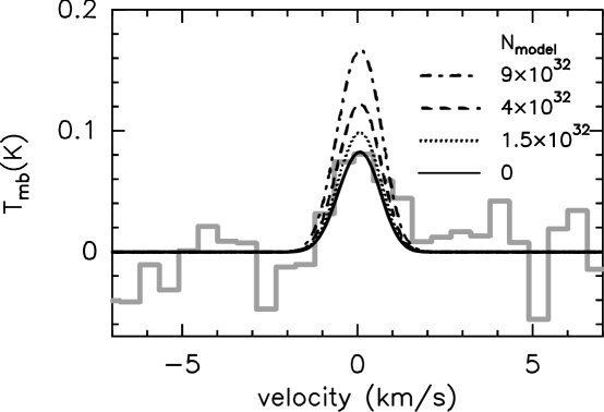
Figure 6: Comparison of SWAS observations and model results for the post-impact period of 4.3 to 6.0 July. The SWAS-observed spectrum is shown as a histogram (weighted average, see text for details). The dashed and dotted lines give the results for outburst models with $\tau=30$ minutes but three different amounts of water in the ejected material. For comparison, the signal expected for a model with a constant water production rate of $Q_{\rm H_{2}O}=5.2\times 10^{27}$ s^-1 is shown as a solid line. The latter is the water production rate of the comet averaged for a 3-day period centered on the impact date.

For a comparison of the SWAS observations to the model, we fit a Gaussian line profile to the observed spectra in each orbital segment after the impact, where we have constrained the fit using the position and width of the line in the model spectrum and only allowed the line intensity to vary. This procedure gives us a line-integrated intensity and a statistical error for the observations made in each orbital segment $i$, $I_{\rm obs,i}\pm\Delta I_{\rm obs,i}$. Note, that no emission line is detected in the spectrum of an individual segment and that the error $\Delta I_{\rm obs,i}$ generally is larger than the integrated intensity from the fit. However, a spectral line of integrated intensity consistent with the pre-impact intensity is detected if $\mathrel{\mathchoice{\vbox{\offinterlineskip\halign{\hfil$\displaystyle#$\hfil\cr>\cr\sim\cr}}}{\vbox{\offinterlineskip\halign{\hfil$\textstyle#$\hfil\cr>\cr\sim\cr}}}{\vbox{\offinterlineskip\halign{\hfil$\scriptstyle#$\hfil\cr>\cr\sim\cr}}}{\vbox{\offinterlineskip\halign{\hfil$\scriptscriptstyle#$\hfil\cr>\cr\sim\cr}}}}25$ segments are co-added. (Fig. 6).

For the evaluation of the post-impact SWAS data, we included observations made up to 42 hrs after the impact. In order to derive an upper limit to the water released by the impact we calculate a weighted average of the SWAS observations, where the spectra in each segment are weighted by the excess intensity resulting from the outburst predicted by the model ($I_{\rm model}-I_{\rm q}$), and by the inverse square of the statistical error of the observed line intensity $(\Delta I_{\rm obs})^{-2}$. The weighted average of the SWAS observations made in several segments allows us to derive a better upper limit than for a single segment, and at the same time avoids that segments where the model predicts a lower intensity are co-added with an equal weight. For a model with a given $\tau$ and $N_{\rm model}$ we first estimate the number of water molecules in the outburst for each individual segment $i$ post-impact by $N_{i}=N_{\rm model}\,(I_{\rm obs,i}-I_{\rm q})/(I_{\rm model,i}-I_{\rm q})$. The accuracy $\Delta N_{i}$ is estimated by standard error propagation of the statistical error of the observed intensity, $\Delta I_{\rm obs,i}$, and of the line intensity before impact, $\Delta I_{\rm q}$. The final estimate for the number of water molecules in the outburst of duration $\tau$ is then calculated as the weighted average of the $N_{i}$,

$$N=\frac{\sum_{i}N_{i}/(\Delta N_{i})^{2}}{\sum_{i}(\Delta N_{i})^{-2}},$$

and the accuracy of this estimate is given by $\Delta N=(\sum_{i}(\Delta N_{i})^{-2})^{1/2}$. The summation is over the orbital segments $i$ after impact. Note, that with $\Delta I_{\rm obs,i}>\Delta I_{\rm q}$ we have $\Delta N_{i}\approx\Delta I_{\rm i,obs}/N_{\rm model}\,(I_{\rm model,i}-I_{\rm q})$ and thus the individual $N_{i}$ are weighted by $(\Delta N_{i})^{-2}\approx(I_{\rm model,i}-I_{\rm q})^{2}/(\Delta I_{\rm i,obs})^{2}$.

The outlined procedure assumes that the excess emission from the outburst is proportional to the number of water molecules in the outburst, whereas optical depth effects mentioned above generally result in a non-linear relation between the number of water molecules in the coma and the detected line intensity. In practice, the upper limit derived from the observations is checked by comparing the results for models with different $N_{\rm model}$, or an iterative process, if needed.

The duration of the outburst following the impact is not known. However, observations suggest that it was relatively short, probably less than a day (Küppers et al., 2005). Assuming an outburst duration $\tau=30$ minutes we obtain $N=(-1.9\pm 2.6)\times 10^{32}$ water molecules for the SWAS observations post impact, and thus a $3\sigma$ upper limit of $5.9\times 10^{32}$ water molecules. Fig. 6 compares a weighted average of the SWAS data post-impact and the model results for four different $N_{\rm model}$. Table 2 lists the results (3$\sigma$ upper limits) for three additional models where we assumed a longer duration for the outburst $\tau=2,8,16$ hrs. The line intensity remains elevated for a longer period in outbursts with $\tau>2$ hrs and the observations of more segments are co-added in this case, resulting in a slightly lower upper limit for the water vapor released by the impact. Therefore, $N<6\times 10^{32}$ molecules ($\sim 1.8\times 10^{7}$ kg) is a conservative upper limit to the water vapor released by the impact.

4 Discussion

No increase in the water rotational-line emission from the impact ejecta was detected by SWAS and we derive a $3$ sigma upper limit to the water vapor generated by the impact, $N_{\rm tot}<6\times 10^{32}$ water molecules ($1.8\times 10^{7}$ kg). The SWAS non-detection is consistent with results from OH observations at UV wavelengths by Küppers et al. (2005) which indicate that only a small amount of water vapor ($\sim 4.5\times 10^{6}$ kg) was produced by the impact and suggest that the dust-to-water ice mass ratio of the ejected material exceeded unity (Keller et al., 2005). However, care has to be taken in arriving at this conclusion. Ice freshly excavated from the impact crater might sublimate rather slowly on exposure to sunlight if the ice was ejected in large chunks, whereas dust ejected into escape orbits by the impact would only linger near the comet for short periods. Early post-impact observations could thus provide a misleading impression of the longer-term integrated dust to water ratio lost by the comet in response to the impact.

No newly formed active area was detected by SWAS to significantly contribute to the water vapor production rate of the comet for more than 2-3 days. The non-detection of water vapor due to the Deep Impact event argues against the impact of meteoritic material as the origin of the natural outbursts observed in 9P/Tempel 1. This is suggested by the small amount of water released by the impact when compared to the natural outbursts, and by the fact that this would require an abundance of meteorites in interplanetary space far higher than all other observations permit in order to explain the number of outbursts observed in 9P/Tempel 1 (eg., Lang, 1992; Ceplecha, 1992; Greenberg et al., 1994, and references therein). Another argument against exogenic processes, such as meteorite impacts, as the reason for the outbursts is the correlation of the outbursts with the light curve observed by A’Hearn et al. (2005).

The water production rate of 9P/Tempel 1 shows large natural variations, and the observed fluctuations are somewhat surprising and difficult to explain. While the surface material of the comet is largely desiccated, periodic spurts of water vapor emission, nevertheless, are observed. Strictly, a model similar to the outburst model presented for the observations made during the Deep Impact event has to be employed for the water monitoring observations, particularly if one considers that the natural outbursts and the overall variability of the water outgassing rate of the comet is much larger than the amount of water vaporized by the impact. While the present paper for the first time presents a model for radio-line emission in outbursting comets, such a modeling is currently computationally prohibitive for the entire data set of the 9P/Tempel 1 observations unless the timing of the outbursts are known (the outburst duration and start time). Several of the strong outbursts recorded by Earth-based instruments are summarized by Meech et al. (2005a), but it is not always possible to exactly constrain the timing of these outbursts because of the limited time coverage of these observations and because tracers other than water were observed in most cases. In fact, the opportunity to correlate observed outburst signals with a well-defined impact date was one of the reasons to conduct the Deep Impact experiment.

For the SWAS observations of a natural outburst, because we average over 2-3 days, it is not possible to decide whether the water molecules were released in a relatively short time ($\tau\ll 3$ days) or at a lower rate over a longer period ($\tau\mathrel{\mathchoice{\vbox{\offinterlineskip\halign{\hfil$\displaystyle#$\hfil\cr<\cr\sim\cr}}}{\vbox{\offinterlineskip\halign{\hfil$\textstyle#$\hfil\cr<\cr\sim\cr}}}{\vbox{\offinterlineskip\halign{\hfil$\scriptstyle#$\hfil\cr<\cr\sim\cr}}}{\vbox{\offinterlineskip\halign{\hfil$\scriptscriptstyle#$\hfil\cr<\cr\sim\cr}}}}$3 days). Presenting an average $Q_{\rm H_{2}O}$ assuming a constant water production rate during the period where the SWAS-detected signal was averaged is therefore acceptable to trace the variation of the cometary activity on time-scales of $\mathrel{\mathchoice{\vbox{\offinterlineskip\halign{\hfil$\displaystyle#$\hfil\cr>\cr\sim\cr}}}{\vbox{\offinterlineskip\halign{\hfil$\textstyle#$\hfil\cr>\cr\sim\cr}}}{\vbox{\offinterlineskip\halign{\hfil$\scriptstyle#$\hfil\cr>\cr\sim\cr}}}{\vbox{\offinterlineskip\halign{\hfil$\scriptscriptstyle#$\hfil\cr>\cr\sim\cr}}}}$days. Since SWAS is sensitive to the total number of water molecules in the extended coma where line excitation is governed by IR-fluorescence, a sudden increase in the water production rate is not immediately visible in the SWAS signal but increases gradually over 1-2 days (Fig. 7). Assuming a two-fold increase of the water production rate, the SWAS-detected signal has reached 90% of the line intensity of the corresponding steady-state model with twice the water production rate within $\sim 30$ hours. Thus, one has to note that the SWAS-derived water production rate for 9P/Tempel 1 presented with Table 1 and Fig. 3) might lag the true water production rate by $\sim 1.3$ days during phases of strong comet variability. A similar conclusion applies to all studies of the water production rate using water-line observations covering a significant fraction of the gaseous coma using a Haser model.

The main indication of desiccation comes from the high surface temperatures and the associated low thermal conductivities and inertia on the sunlit side of the comet. A’Hearn et al. (2005) find that 9P/Tempel 1 has a largely homogeneous color and uniform albedo as low as $0.04\pm 0.02$ over its entire surface. At perihelion, maps of the nucleus show temperature variations across the surface between $260\pm 6$ K to $329\pm 8$ K, with an absolute calibration uncertainty of order 20%. Even at the lowest cited temperature, however, the sublimation rate of ice close to the comet surface would be significantly higher than observed. As A’Hearn et al. (2005) also point out, the high surface temperature argues for a thermal inertia probably lower than $10^{5}$ erg K^-1 cm^-2 s^-1/2. This implies that the 40.83 hr periodic heat pulse on the sunlit side corresponding to the observed 40.83 hr rotation period observed close to perihelion does not penetrate deep into the comet’s surface, and is consistent with the low intra-pulse evaporation rate of water. Most of the frozen water apparently resides deeper beneath the surface than the heat pulse penetrates, and remains at a temperature sufficiently low to limit sublimation. Sunshine et al. (2006) detect water ice on the surface of 9P/Tempel 1, but these ice deposits cover too small a fraction of the surface to account for the total water vaporization rate observed for the comet.

A less compelling indication for dehydration of the comet’s surface layers comes from the debris released by the July 4 impact. A’Hearn et al. (2005) conclude that ejecta consisted largely of very fine dust in the 1 to 100 micrometer size range, while Meech et al. (2005a) find the ratio of dust to gas in the impact ejecta to have been significantly higher than in the pre-impact emission of material from the comet. Meech et al. (2005a) show that the light curve mainly associated with dust emission rose to a maximum within roughly half an hour after impact and then declined after two hours, Mumma et al. (2005) estimate a doubling of the post-impact water vapor production rate integrated over a 24 hour period. A contribution to the water vapor production over this longer period could have come from newly excavated material ejected from the crater and strewn over a sizeable surrounding area, consistent with the observation that an appreciable fraction of the excavated material fell back onto the comet surface. The ice in the ejecta would subsequently have been sublimated by sunlight. As Küppers et al. (2005) point out, the heat required for the evaporation of this much water could not have been provided by the energy of impact and would instead have had to come from the Sun.

A’Hearn et al. (2005) point out that a number of pre-impact cometary outbursts appear to be correlated with the comet’s rotation rate. More specifically, they identify emission from a topographic feature, possibly a scarp or depression, that sees the sun rising around the time of each outburst. The sudden heating of the surface of the topographic feature by direct sunlight could cause both rapid sublimation and the release of dust grains no longer held together by ice. Smaller grains could be carried off into space by the evaporating water. The gravitational attraction of the comet is sufficient to have retained a significant fraction of the solid impact ejecta, as shown by the plume of material raining back down onto the comet’s surface after impact.

The SWAS water vapor detection history shown in Fig. 3 indicates a rough correlation between the times of a natural outburst identified by other observers, and a rise in the 557 GHz water vapor emission integrated over a day or two following the outburst. This time delay is consistent with the expected response of the SWAS-detected signal to an instant increase of the water vaporization rate of the nucleus shown in Fig. 7. In this context it should be noted that the outbursts indicated in Fig. 3 are “big” natural outburst which were also detected by Earth-based telescopes, while the weaker outbursts reported by A’Hearn et al. (2005) were too faint to be detected by Earth-based instruments.

If the prime source of water vapor is a tilted topographic feature on the surface such as a scarp or wall, and the outburst occurs at sunrise, a slight slowing down of the comet’s rotation should become evident in the course of time. The momentum of evaporating water along the direction of rotation is $\sim N(mkT)^{1/2}$, where $N$ is the total number of water molecules released over a period of time, $T\sim 300$ K is the surface temperature at sunrise and $m$ is the molecular weight of water. With a lower limit to the number of water molecules vaporized from the nucleus during the 2005 perihelion passage of $N\sim 10^{35}$ (Sect. 3.2), the net angular momentum transferred to the comet nucleus through evaporation at radius $r\sim 3$ km should have been roughly $N(mkT)^{1/2}r\sim 3\times 10^{22}$g cm² s^-1. The angular momentum of the comet is $\sim\pi Mr^{2}/P$, where $P\sim 40.83\pm 0.33$ hr is the rotation period, $M\sim 4\pi\rho r^{3}/3$ and $\rho\sim 0.6$ g cm^-3 is the density of the nucleus cited by A’Hearn et al. (2005). For comet 9P/Tempel 1, $\pi Mr^{2}/P\sim 2\times 10^{23}$ g cm² s^-1. While the fractional mass lost by the comet due to the sublimation of ice is quite small, the velocity of sublimated molecules is several thousand times higher than the rotational surface velocity of the comet. A systematic change in the rotational period of the comet could, therefore, amount to as much as several percent during a single perihelion passage.

Whether a slowdown in the comet’s rotational period by up to a few percent during the 2005 perihelion passage could be culled out from the data is not clear. Belton et al. (2005) give the pre-perihelion rotation period of the comet at heliocentric distances greater than 4 AU as $41.85\pm 0.10$ hours, although it is not clear whether this significantly differs from the 40.83 hours measured at perihelion. If so, the comet’s rotation rate appears to have sped up during perihelion passage. Either way, it would be useful to re-measure the post-perihelion rotation period at large heliocentric distances to see whether significant changes in the rotation period of Tempel 1 can be established.

Observations and Water Vaporization Rate Date $r_{h}$ $\Delta$ $I_{\rm mb}=\int T_{\rm mb}\,dv$ $Q_{\rm H_{2}O}$ (AU) (AU) (K km s^-1) ($10^{28}\,s^{-1}$) Jun 5-9 1.53 0.78 $0.193\pm 0.041$ $0.63\pm 0.13$ Jun 10-11 1.53 0.79 $0.304\pm 0.067$ $1.02\pm 0.22$ Jun 12-13 1.52 0.80 $0.334\pm 0.053$ $1.12\pm 0.18$ Jun 14-15 1.52 0.81 $0.382\pm 0.073$ $1.29\pm 0.25$ Jun 18-19 1.52 0.82 $0.352\pm 0.079$ $1.21\pm 0.27$ Jun 20-21 1.51 0.83 $0.106\pm 0.039$ $0.38\pm 0.13$ Jun 22-23 1.51 0.84 $0.149\pm 0.041$ $0.54\pm 0.14$ Jun 24-25 1.51 0.85 $0.273\pm 0.059$ $0.98\pm 0.21$ Jun 26-27 1.51 0.86 $0.286\pm 0.064$ $1.05\pm 0.23$ Jun 28-30 1.51 0.87 $0.127\pm 0.044$ $0.49\pm 0.16$ Jul 1-3 1.51 0.89 $0.163\pm 0.038$ $0.66\pm 0.15$ Jul 2.7-5.7 1.51 0.89 $0.121\pm 0.036$ $0.52\pm 0.15$ Jul 4-6 1.51 0.90 $0.164\pm 0.038$ $0.69\pm 0.16$ Jul 7-9 1.51 0.92 $0.221\pm 0.050$ $0.98\pm 0.20$ Jul 10-23 1.51-1.52 0.93-1.01 $0.067\pm 0.022$ $0.32\pm 0.12$ Jul 24-27 1.52 1.01-1.03 $0.133\pm 0.044$ $0.67\pm 0.21$ Jul 28-30 1.53 1.03-1.07 $0.169\pm 0.041$ $0.90\pm 0.21$ Jul 30-Aug 4 1.53-1.54 1.05-1.10 $<0.135$ $<0.75$ Aug 5-10 1.54 1.10-1.14 $0.084\pm 0.024$ $0.49\pm 0.14$ Aug 10-17 1.55-1.57 1.14-1.20 $<0.092$ $<0.58$ Aug 18-20 1.57-1.58 1.20-1.23 $0.154\pm 0.034$ $1.03\pm 0.23$ Aug 21-23 1.58 1.23-1.25 $0.125\pm 0.042$ $0.98\pm 0.32$ Aug 24-Sep 1 1.59-1.61 1.25-1.35 $<0.094$ $<0.72$ Jun 5-Jul 3 1.53-1.51 0.78-0.89 $0.225\pm 0.017$ $0.81\pm 0.06$ Jul 10-Aug 7 1.51-1.54 0.93-1.11 $0.065\pm 0.017$ $0.34\pm 0.08$ Aug 8-Sep 1 1.54-1.61 1.12-1.35 $0.074\pm 0.015$ $0.52\pm 0.10$

Table 1: SWAS monitoring and water vaporization rate of comet 9P/Tempel 1. In columns 4 and 5, the error bars are one sigma and upper limits are 3 sigma.

Total Water released by the Impact
Burst Duration Upper limit (Model) $\tau$ (hrs) $N$ (molec.) 0.5 $<5.9\times 10^{32}$ 2.0 $<6.1\times 10^{32}$ 8.0 $<5.3\times 10^{32}$ 16.0 $<3.9\times 10^{32}$

Table 2: SWAS-derived upper limits on the water released by the impact. The $3\sigma$ upper limit is given for the assumed duration $\tau$ of the outburst

Figure 1: SWAS-measured ground-state 556.936 GHz ortho-water line toward comet 9P/Tempel 1. The spectrum shows emission observed between 10 June and 19 June and the line represents approximately 24 hrs of on-source integration. The velocity scale of the reduced data is given in the rest-frame of the comet.

Figure 2: SWAS observation of the $1_{10}\rightarrow 1_{01}$ ground-state transition of ortho water. The average spectrum is shown respectively for the period of 14.03-19.99 June 2005 (left) and 20.00-24.00 June 2005 (right).

Figure 3: Top panel: Comet-Sun distance ($r_{\rm h}$) and Comet-Earth distance ($\Delta$) for 9P/Tempel 1 for the period of June through August 2005. Bottom panel: total water production rate $Q_{\rm H_{2}O}$ derived from SWAS observations of the $1_{10}\rightarrow 1_{01}$ transition of ortho water. The impact date is marked by the vertical line. Outbursts reported from observations at other wavelengths are marked by filled triangles (Meech et al., 2005a). Note, that the clustering of open triangles in June and July 2005 does not necessarily indicate that the comet was more active during this period. Rather, it likely results from observational bias, since most of the observing campaigns for 9P/Tempel 1 had been conducted during the days leading up to and immediately following the Deep Impact encounter with the comet on 4 July.

Figure 4: SWAS spectra of 9P/Tempel 1, respectively, averaged over a period of 3 days before and after the impact.

Figure 5: Velocity-integrated intensity calculated for four different outburst models (see legend at top right). Open symbols show three models with an outburst duration of $\tau=$30 min but a different amount of water released by the outburst. The filled symbols give the results for a model with $\tau=8$ hrs. The pre-outburst level $I_{q}=0.121$ K km s^-1 is indicated by the dotted horizontal line.

Figure 7: Response of the SWAS-detected line intensity (bottom panel) to an instant, two-fold increase of the water production rate (top panel). The lower panel shows the evolution of the line-integrated intensity if the water production rate of the comet is increased from 5.2 to 10.4$\times 10^{27}$ s^-1 at $t=0$. (The vertical lines give the line intensity for a steady-state model with these water production rates). This model is applicable to a situation where a new active area is created, for example, following an impact or a splitting of a comet nucleus. Other model parameter ($r_{\rm h},\Delta,v_{\rm exp}$) are those applicable to 9P/Tempel 1 on 4 June 2005.