Dark matter clustering: a simple renormalization group approach

Abstract

I compute a renormalization group (RG) improvement to the standard beyond-linear-order Eulerian perturbation theory (PT) calculation of the power spectrum of large-scale density fluctuations in the Universe. At $z=0$, for a power spectrum matching current observations, lowest order RGPT appears to be as accurate as one can test using existing numerical simulation-calibrated fitting formulas out to at least $k\simeq 0.3\,h\,{\rm Mpc}^{-1}$; although inaccuracy is guaranteed at some level by approximations in the calculation (which can be improved in the future). In contrast, standard PT breaks down virtually as soon as beyond-linear corrections become non-negligible, on scales even larger than $k=0.1\,h\,{\rm Mpc}^{-1}$. This extension in range of validity could substantially enhance the usefulness of PT for interpreting baryonic acoustic oscillation surveys aimed at probing dark energy, for example. I show that the predicted power spectrum converges at high $k$ to a power law with index given by the fixed-point solution of the RG equation. I discuss many possible future directions for this line of work. The basic calculation of this paper should be easily understandable without any prior knowledge of RG methods, while a rich background of mathematical physics literature exists for the interested reader.

I Introduction

Statistics of the large-scale density fluctuations in the Universe provide an invaluable source of information on the very early Universe, where the initial density perturbations that grow by gravitational instability were created, and on the material content and gravitational laws of the Universe, which determine the growth of structure and how it looks to us from a distance (Seljak et al., 2006). The standard practical toolbox we use for interpreting observations consists of linear theory on very large scales or at very early times (Seljak and Zaldarriaga, 1996), and everywhere else numerical simulations which compute the fully non-linear evolution of a realization of the density field in a patch of Universe. Fitting formulas, motivated by physical intuition but ultimately heuristic, are often used to more efficiently interpolate between simulation results (Smith et al., 2003; Warren et al., 2006).

Beyond linear order perturbation theory (PT) has been considered for a long time (Peebles, 1980; Juszkiewicz, 1981; Vishniac, 1983; Fry, 1984; Goroff et al., 1986; Jain and Bertschinger, 1994; Scoccimarro and Frieman, 1996), but does not currently play an important role in our interpretation of precision observations (see Bernardeau et al. (2002) for a thorough review of large-scale structure perturbation theory). The desire to measure dark energy properties using observations of baryonic acoustic oscillation features (Eisenstein et al., 1998; Eisenstein and Hu, 1998; Cooray et al., 2001; Eisenstein, 2003; Blake and Glazebrook, 2003; Linder, 2003; Seo and Eisenstein, 2003; Matsubara, 2004; Glazebrook and Blake, 2005; Glazebrook et al., 2005; Amendola et al., 2005; Blake and Bridle, 2005; Blake et al., 2006; Dolney et al., 2006; McDonald and Eisenstein, 2006), which fall more or less exactly in the range of scales where higher order perturbation theory could be most useful, gives this line of work much more pressing practical relevance than it has had in the past (Jeong and Komatsu, 2006). More traditional uses of galaxy clustering to measure cosmological parameters, long reliant on the assumption that galaxy power is simply proportional to linear mass power, have also reached the point where weakly non-linear effects are a substantial limitation (Tegmark et al., 2004; Sánchez et al., 2006). Additionally, other probes of large-scale structure, like the Ly$\alpha$ forest (McDonald et al., 2005; Viel and Haehnelt, 2006), weak lensing (Hoekstra et al., 2006), galaxy cluster/Sunyaev-Zel’dovich effect (SZ) measurements (DeDeo et al., 2005), and possibly future 21cm surveys (Nusser, 2005), could all benefit from improved computational techniques.

The problem with higher order perturbation theory is that it does not work very well in exactly the regime where it could currently be most useful: at low redshift and wavenumber $k\sim 0.1\,h\,{\rm Mpc}^{-1}$, where galaxy clustering is significantly but still only weakly non-linear (Scoccimarro, 2004). Recently, Crocce and Scoccimarro (2006a, b) proposed a renormalization technique aimed at improving PT calculations. They re-sum an infinite series of perturbation theory terms (Feynman diagrams) which determine the memory of perturbations to initial conditions as a function of scale (see also Scoccimarro (2001)). This method is apparently computationally difficult because they have not yet computed a power spectrum using it. The renormalization group (RG) method I present here is different, but surely related. There has been some work toward using RG techniques to model large-scale structure (Barbero G. et al., 1997; Domínguez et al., 1999; Gaite, 2001). The methods used are different than mine, and have not yet seen much practical application for comparison with observations.

My implementation of the RG is inspired more by its use for dealing with secular divergences in perturbative solutions of differential equations (Chen et al., 1994, 1996) than by the probably better known applications in high energy and statistical physics (Wilson and Kogut, 1974; Wilson, 1983; Shankar, 1994; Berges et al., 2002), although all of these uses are related. The basic idea is to identify a quantity in the problem that is not directly observable and modify it to remove breakdowns in the perturbation theory, leading to a well-behaved renormalized observable. In this paper I renormalize the initial (linear theory) power spectrum to remove the relative (not actually infinite for realistic power spectra) divergence of the lowest order correction to linear theory. More detailed mathematical clarification and explanation of the meaning of the method of Chen et al. (1994, 1996), in terms of the theory of envelopes, can be found in Kunihiro (1995, 1997). Even more detailed treatments can be found in (Shirkov and Kovalev, 2001; Kovalev and Shirkov, 2006). These papers should be useful to the reader who is unsatisfied with my presentation, or wants to extend it. During the last several years, Boyanovsky et al. (1999); Boyanovsky and de Vega (1999); Boyanovsky et al. (2000); Wang et al. (2000); Boyanovsky et al. (2002, 2003); Boyanovsky and de Vega (2003) have extended and generalized this dynamical renormalization group method to compute the real time evolution of expectation values of quantum fields.

The rest of the paper is as follows: In §II I derive a simple formula for the RG-improved power spectrum of mass density fluctuations. In §III I show numerical results and compare them to standard PT and fitting formulas calibrated using simulations. Finally, in §IV I discuss possible future directions for this kind of work.

II Calculation

In this section I present the basic calculation. In §II.1 I discuss the time evolution equations for cold dark matter, which are the starting point for perturbation theory. In §II.2 I review standard Eulerian perturbation theory. Finally, in §II.3 I apply the renormalization group improvement.

II.1 Evolution equations

We are interested in the statistics of the mass density field, $\delta(\mathbf{x},\tau)=\rho(\mathbf{x},\tau)/\bar{\rho}-1$, with Fourier transform $\delta(\mathbf{k},\tau)=\int d^{3}\mathbf{x}~{}\exp(i\mathbf{k}\cdot\mathbf{x})~{}\delta(\mathbf{x},\tau)$, where $\mathbf{x}$ is the comoving position and $\tau=\int dt/a$ is the conformal time, with $a=1/(1+z)$ the expansion factor. In particular, I will compute the power spectrum, $P(k,\tau)$, defined by

$$\left<\delta(\mathbf{k},\tau)\delta(\mathbf{k}^{\prime},\tau)\right>=(2\pi)^{3}\delta_{D}(\mathbf{k}+\mathbf{k}^{\prime})P(k,\tau)$$ (1)

For now I will assume only cold dark matter, i.e., collisionless particles with insignificant initial velocity dispersion. The exact evolution is is described by the Vlasov equation (Peebles, 1980)

$$\frac{\partial f}{\partial\tau}+\frac{1}{a~{}m}~{}\mathbf{p}\cdot\mathbf{\nabla}f-a~{}m~{}\mathbf{\nabla}\phi\cdot\mathbf{\nabla}_{\mathbf{p}}f=0~{},$$ (2)

with

$$\nabla^{2}\phi=4~{}\pi~{}G~{}a^{2}\bar{\rho}~{}\delta~{},$$ (3)

where $f(\mathbf{x},\mathbf{p},\tau)$ is the particle density at phase-space position $(\mathbf{x},\mathbf{p})$, $m$ is the particle mass (which plays no role in the final results), and $\mathbf{p}=a~{}m\mathbf{v}$ ($\mathbf{v}$ here is a particle’s peculiar velocity, not to be confused with the mean peculiar velocity of all particles at some point in space, used everywhere else). Except when otherwise indicated $\mathbf{\nabla}=\mathbf{\partial/\partial x}$. The density field is obtained by averaging the distribution function over momentum:

$$\rho(\mathbf{x},\tau)=ma^{-3}\int d^{3}p~{}f(\mathbf{x},\mathbf{p},\tau)~{},$$ (4)

and the bulk (mean) velocity and higher moments of the velocity distribution e.g., the dispersion of particle velocities around their bulk velocity, can be similarly obtained by multiplying the distribution function by any number of $\mathbf{p}$’s (e.g., one to obtain bulk velocity) before integrating over $\mathbf{p}$. As discussed by Peebles (1980), taking moments of the Vlasov equation with respect to momentum leads to a hierarchy of evolution equations for these quantities. Dropping the higher moments of the velocity distribution gives the usual hydrodynamic equations for density and bulk velocity:

$$\frac{\partial\delta}{\partial\tau}+\mathbf{\nabla}\cdot\left[\left(1+\delta\right)\mathbf{v}\right]=0~{},$$ (5)

and

$$\frac{\partial\mathbf{v}}{\partial\tau}+\mathcal{H}\mathbf{v}+\left(\mathbf{v}\cdot\mathbf{\nabla}\right)\mathbf{v}=-\mathbf{\nabla}\phi~{},$$ (6)

where $\mathcal{H}=d\ln a/d\tau=aH$ with $H$ the usual Hubble parameter.

II.2 Standard Eulerian perturbation theory

Perturbation theory consists of writing the density and velocity fields as a series of terms of at least formally increasing order of smallness, i.e., $\delta=\delta_{1}+\delta_{2}+\delta_{3}+...$. The evolution equations are solved order-by-order, with lower order solutions appearing as sources in the higher order equations so that $\delta_{n}$ is of order $\delta_{1}^{n}$ (Bernardeau et al., 2002). The power spectrum for Gaussian initial conditions is given by

$$\left<\delta(\mathbf{k})\delta(\mathbf{k}^{\prime})\right>=\left<\delta_{1}(\mathbf{k})\delta_{1}(\mathbf{k}^{\prime})\right>+\left<\delta_{1}(\mathbf{k})\delta_{3}(\mathbf{k}^{\prime})\right>+\left<\delta_{3}(\mathbf{k})\delta_{1}(\mathbf{k}^{\prime})\right>+\left<\delta_{2}(\mathbf{k})\delta_{2}(\mathbf{k}^{\prime})\right>+...$$ (7)

where no terms 3rd order in $\delta_{1}$ appear because the expectation value of any term cubic in a Gaussian field is zero.

At this point I assume an Einstein-de Sitter Universe for simplicity, and define

$$P(k,\tau)=D^{2}(\tau)P_{11}(k)+D^{4}(\tau)\left[P_{13}(k)+P_{22}(k)\right]+...~{},$$ (8)

where $D(\tau)=\delta_{1}(\tau)/\delta_{\rm initial}$ is the linear theory growth factor. The Einstein-de Sitter assumption is needed to avoid more complicated time dependence of $P_{13}$ and $P_{22}$, but the real Universe is of course not Einstein-de Sitter. Fortunately, this is not a significant problem because, to percent level accuracy (Martel and Freudling, 1991; Bouchet et al., 1992; Bernardeau, 1994; Bouchet et al., 1995; Matsubara, 1995; Catelan et al., 1995; Scoccimarro et al., 1998; Jeong and Komatsu, 2006), the effect of changing the background model can be included by simply using the correct linear growth factor in Eq. (8). I will sometimes refer to $P_{13}$ and $P_{22}$ as 2nd order, meaning in the initial power spectrum amplitude, not to be confused with the fact that they are 4th order in $\delta_{1}$ and require calculating the evolution of $\delta$ to 3rd order, i.e., $\delta_{3}$. Makino et al. (1992) derived the following useful form of the equations for $P_{13}(k)$ and $P_{22}(k)$:

$$P_{13}(k)=\frac{k^{3}P_{11}(k)}{252\left(2\pi\right)^{2}}\int_{0}^{\infty}drP_{11}(kr)\left[\frac{12}{r^{2}}-158+100r^{2}-42r^{4}+\frac{3}{r^{3}}\left(r^{2}-1\right)^{3}(7r^{2}+2)\ln\left|\frac{1+r}{1-r}\right|\right]$$ (9)

and

$$P_{22}(k)=\frac{k^{3}}{98\left(2\pi\right)^{2}}\int_{0}^{\infty}drP_{11}\left(kr\right)\int_{-1}^{1}dxP_{11}\left[k\left(1+r^{2}-2rx\right)^{1/2}\right]\frac{\left(3r+7x-10rx^{2}\right)^{2}}{\left(1+r^{2}-2rx\right)^{2}}~{}.$$ (10)

Note that, due to many cancellations, these terms are not as divergent as they might appear at first glance, their sum being convergent at high $k$ for power law $P_{11}(k)$ with $n=d\ln P/d\ln k<-1$ and at low $k$ when $n>-3$ (Makino et al., 1992). Their sum is zero for $n\simeq-1.4$ (Bernardeau et al., 2002), a fact that will have interesting consequences for our RG calculation.

II.3 Renormalization group improvement

The problem with the standard calculation outlined in §II.2, which leads us to renormalization, is that the 2nd term in Eq. (8) diverges relative to the first (although it does not literally become infinite for realistic power spectra), at increasingly large scales (small $k$) as time progresses. This divergence is not exactly unphysical – we expect non-linearities to become important during gravitational collapse – however, the basic premise of perturbation theory is violated when higher order terms become large. There is no a priori reason to expect the results to be accurate. I employ a renormalization group calculation to cure this divergence. I start in §II.3.1 with a quick derivation motivated by the method of Chen et al. (1994). Then I discuss the mathematical background, physical interpretation, approximations, and limitations of the method in §II.3.2.

II.3.1 Simple calculation

To simplify the presentation of the calculation, I rewrite Eq. (8) in a more compact, schematic form,

$$\tilde{P}(k,\tau)\simeq P_{L}(k)+A~{}\left[P_{L}^{2}\right](k)~{},$$ (11)

where $A\propto D^{2}(\tau)$, $\tilde{P}(k,\tau)\equiv P(k,\tau)/A$, $P_{L}(k)$ is the initial condition power, and $[P_{L}^{2}](k)\equiv P_{13}(k)+P_{22}(k)$ is the higher order correction term, which is quadratic in $P_{L}(k)$, as given by Eqs. (9) and (10). I now follow the method described in Chen et al. (1994) to deal with the problem of the 2nd order term becoming large (deferring a detailed explanation of the meaning of this method to §II.3.2). I rewrite $A=A-A_{\star}+A_{\star}$, where $A_{\star}$ is just an arbitrary constant, so that

$$\tilde{P}(k,\tau)=P_{L}(k)+A_{\star}\left[P_{L}^{2}\right](k)+(A-A_{\star})\left[P_{L}^{2}\right](k)~{}.$$ (12)

I then absorb the constant $A_{\star}\left[P_{L}^{2}\right](k)$ into the initial conditions, $P_{L}(k)$, defining the renormalized initial conditions $P_{\star}(k,A_{\star})$, so that

$$\tilde{P}(k)=P_{\star}(k,A_{\star})+(A-A_{\star})\left[P_{\star}^{2}\right](k)~{},$$ (13)

where I can freely replace $P_{L}$ with $P_{\star}$ in the 2nd term because the change is formally 3rd order (in the initial power spectrum amplitude). The observable power spectrum $\tilde{P}(k)$ obviously must be independent of the completely artificial constant $A_{\star}$, so I impose $d\tilde{P}(k)/dA_{\star}=0$ and find

$$\frac{dP_{\star}(k,A_{\star})}{dA_{\star}}=\left[P_{\star}^{2}\right](k)~{},$$ (14)

where I have dropped the derivative of $\left[P_{\star}^{2}\right](k)$ because it is higher order (this is seen to be self-consistent from Eq. 14 itself). This equation is easy enough to solve numerically, given $P_{\star}(k,A_{\star})$ at some value of $A_{\star}$. Since $A_{\star}$ is completely arbitrary, I will in the end choose $A_{\star}=A$, removing the 2nd term in Eq. (13) entirely. The result for $\tilde{P}(k,\tau)$ is then simply $P_{\star}(k,A_{\star}=A)$, obtained by solving Eq. (14). To reproduce the linear theory result at very early times, the initial conditions for the solution of Eq. (14) must be $P_{\star}(k,A_{\star}=0)=P_{L}(k)$.

II.3.2 Explanation

The method of Chen et al. (1994) and related papers was, by the authors own admission, somewhat lacking in rigorous motivation. This situation was clarified by others Kunihiro (1995, 1997); Shirkov and Kovalev (2001); Kovalev and Shirkov (2006); however, their explanations may be opaque. A very simple example should serve to explain and clarify the method. Consider the differential equation

$$\dot{\delta}=\delta+\delta^{2}.$$ (15)

The exact solution is easy to obtain, but suppose one did not know that and solved Eq. (15) using perturbation theory for small initial $\delta$, as in the cosmological situation. The solution to the linearized equation is $\delta_{1}=g_{1}e^{t}$. The equation for the first non-linear correction, $\delta_{2}$, is then

$$\dot{\delta}_{2}=\delta_{2}+g_{1}^{2}e^{2t}$$ (16)

with solution

$$\delta_{2}=g_{2}e^{t}+g_{1}^{2}e^{2t}.$$ (17)

The approach generally followed in the cosmological case is to set the term that is the solution to the homogeneous equation, $g_{2}e^{t}$, to zero, i.e., to assume that at asymptotically early times $\delta\rightarrow\delta_{1}$; however, this is a choice, not necessary. The key observation here is that solving two differential equations has produced two parameters in the solution, $g_{1}$ and $g_{2}$, but we only need one to satisfy the physical boundary conditions. The RG method exploits and fixes the otherwise arbitrary extra parameter of the perturbative solution (note that this approach gives exactly the same result as the approach of “splitting” the linear solution into two pieces, one of which is considered to be second order and used to cancel the non-linear correction).

For the standard choice $g_{2}=0$, $\delta_{2}$ inevitably becomes larger than $\delta_{1}$, invalidating the perturbation theory. Note, however, that using $g_{2}$ we can actually guarantee that at any one chosen time, $t_{\star}$, $\delta_{2}(t_{\star})=0$, and very near $t_{\star}$, $\delta_{2}\ll\delta_{1}$. This requires $g_{2}=-g_{1}^{2}e^{t_{\star}}$, which leads to full solution

$$\delta\simeq g_{1}e^{t}+g_{1}^{2}e^{t}(e^{t}-e^{t_{\star}}).$$ (18)

Clearly the value of $g_{1}$ must depend on the choice of $t_{\star}$, i.e., $g_{1}=g_{1}(t_{\star})$, for a fixed physical situation (fixed full solution $\delta(t)$); however, nothing would be accomplished by simply fixing $g_{1}(t_{\star})$ to match the initial conditions, because this generally requires using the perturbative solution outside its range of validity. The RG method is to determine $g_{1}(t_{\star})$ by enforcing the idea that the physical solution should be independent of the arbitrary time $t_{\star}$, while using the perturbative solution only for $t$ infinitesimally close to $t_{\star}$, where it should be valid, i.e.,

$$\left.\frac{d\delta(t)}{dt_{\star}}\right|_{t_{\star}=t}=0=\frac{dg_{1}(t)}{dt}e^{t}-g_{1}^{2}e^{2t}$$ (19)

or

$$\frac{dg_{1}(t)}{dt}=g_{1}^{2}e^{t}$$ (20)

The exact solution to this equation is $g_{1}(t)=c/(1-ce^{t})$ where $c$ is a constant which will allow matching of the physical initial conditions. Finally, referring back to Eq. (18), evaluated at $t_{\star}=t$, gives the final solution

$$\delta(t)=\frac{ce^{t}}{1-ce^{t}}.$$ (21)

While such good fortune would generally not be expected, it happens that this is the exact solution to the original differential equation, Eq. (15).

The intuitive picture one should have of this calculation is of stepping forward in time slightly using the perturbative solution centered at the present time, then taking the result and using it as the initial condition for a perturbative solution around the new time, followed by another step, and so on. Kunihiro (1995) showed that this method gives the envelope equation for the set of solutions obtained by applying the perturbation theory near various times $t_{\star}$ (the envelope is the curve which is tangent to each of the different solutions).

To make the analogy with original case of the power spectrum clear, note that changing variables to $A=\exp\left(t\right)$, $A_{\star}=\exp\left(t_{\star}\right)$, and $\tilde{\delta}=\delta/A$ in Eq. (18) produces an equation with the same form as Eq. (13). The rest of the derivation follows identically until, unfortunately, Eq. (14) is not analytically solvable because $P(k)$ represents an infinite number of variables rather than one.

While the resulting equations look similar, the skeptical reader may still question the relation between the derivation of Eq. (14) for the power spectrum and Eq. (20) for a single variable governed by a differential equation, e.g., $\delta$ would be most naturally be identified with the cosmological density field, not the power spectrum. To complete the connection one must return to the original derivation of cosmological perturbation theory. At linear order $\delta_{1}(\mathbf{k})=D~{}g_{1}(\mathbf{k})$ where $g_{1}(\mathbf{k})$ is the normalization and $D=a$ is the growth factor (assuming an EdS Universe as usual), and I have dropped the decaying mode solution as usual (I will discuss this further below). At 2nd order

$$\delta_{2}(\mathbf{k})=D~{}g_{2}(\mathbf{k})+D^{2}\int\frac{d^{3}\mathbf{q}}{\left(2\pi\right)^{3}}g_{1}(\mathbf{q})g_{1}(\mathbf{k}-\mathbf{q})J_{S}^{(2)}(\mathbf{q},\mathbf{k}-\mathbf{q})~{},$$ (22)

where the $D~{}g_{2}(\mathbf{k})$ term is set to zero in the standard calculation (see Heavens et al. (1998) for explicit forms of $J_{S}^{(2)}$ and $J_{S}^{(3)}$ below). Again, this equation is missing terms which grow like $D^{-1/2}$ or slower (naively one would expect them to be unimportant).

$\delta_{3}$ is needed to compute the power spectrum, but computing the bispectrum at this point is informative:

$$\left<\delta(\mathbf{k}_{1})\delta(\mathbf{k}_{2})\delta(\mathbf{k}_{3})\right> = D^{3}\left<g_{1}(\mathbf{k}_{1})g_{1}(\mathbf{k}_{2})g_{1}(\mathbf{k}_{3})\right>+D^{3}\left<g_{2}(\mathbf{k}_{1})g_{1}(\mathbf{k}_{2})g_{1}(\mathbf{k}_{3})\right>$$ (23)

$$+ D^{4}\int\frac{d^{3}\mathbf{q}}{\left(2\pi\right)^{3}}J_{S}^{(2)}(\mathbf{q},\mathbf{k}_{1}-\mathbf{q})\left<g_{1}(\mathbf{q})g_{1}(\mathbf{k}_{1}-\mathbf{q})g_{1}(\mathbf{k}_{2})g_{1}(\mathbf{k}_{3})\right>+{\rm cyclic~{}permutations~{}of}~{}\mathbf{k}_{i}~{}.$$

The last term here is the usual perturbative result. The first term is normally zero, for Gaussian initial conditions. The middle term is normally zero because $g_{2}(\mathbf{k})$ is chosen to be zero. One can look at Eq. (23) two ways: The easy way is to say that there is no breakdown in perturbation theory, where a higher order term becomes larger than a lower order term. The last term is the leading term, i.e., the bispectrum is fundamentally $\mathcal{O}\left(\delta_{1}^{4}\right)$, and there is no need for the first two terms to enter this discussion at all. The second approach is to argue that all possible terms should be included in the calculation – the fact that the first term happens to be zero initially is a peculiarity of the initial conditions, not fundamental to the calculation. In this approach, the new middle term, since it is arbitrary, could be set in a way that would cancel the last term at some chosen $D_{\star}$. The first term becomes a function of $D_{\star}$, and requiring that the solution be independent of $D_{\star}$ would produce an RG equation for $\left<g_{1}(\mathbf{k}_{1})g_{1}(\mathbf{k}_{2})g_{1}(\mathbf{k}_{3})\right>(D_{\star})$, just as above in the simple example. The second approach is clearly more thorough, however, in this paper I will take the easy route and declare the usual bispectrum term to be the leading order, with no need for renormalization, i.e., I will set $g_{2}(\mathbf{k})\equiv 0$ as usual (we will see that this term is not needed to renormalize the power spectrum). While my approach may not give the best possible result, it is not fundamentally incorrect, at least not any more than standard perturbation theory is fundamentally incorrect. Renormalization is a tool, not an imperative, and renormalizing part of the calculation but not all of it should be better than nothing.

Moving on to $\delta_{3}$, and again including the homogeneous solution, gives

$$\delta_{3}(\mathbf{k})=Dg_{3}(\mathbf{k})+D^{3}\int\frac{d^{3}\mathbf{q}_{1}}{\left(2\pi\right)^{3}}\frac{d^{3}\mathbf{q}_{2}}{\left(2\pi\right)^{3}}g_{1}(\mathbf{q}_{1})g_{1}(\mathbf{q}_{2})g_{1}(\mathbf{k}-\mathbf{q}_{1}-\mathbf{q}_{2})J_{S}^{(3)}(\mathbf{q}_{1},\mathbf{q}_{2},\mathbf{k}-\mathbf{q}_{1}-\mathbf{q}_{2})~{},$$ (24)

where terms that grow like $D^{1/2}$ or slower have as usual been dropped. The power spectrum is now

$$\left<\delta(\mathbf{k}_{1})\delta(\mathbf{k}_{2})\right>=D^{2}\left<g_{1}(\mathbf{k}_{1})g_{1}(\mathbf{k}_{2})\right>+D^{2}\left<g_{3}(\mathbf{k}_{1})g_{1}(\mathbf{k}_{2})+g_{1}(\mathbf{k}_{1})g_{3}(\mathbf{k}_{2})\right>+D^{4}(2\pi)^{3}\delta^{D}(\mathbf{k}_{1}+\mathbf{k}_{2})[g_{1}^{4}](k_{1})$$ (25)

where $[g_{1}^{4}](k)\equiv P_{13}(k)+P_{22}(k)$ is, as $[P_{L}^{2}](k)$ above, just a quick way of writing the usual $\mathcal{O}\left(\delta_{1}^{4}\right)$ perturbative correction terms (note that if I had promoted the leading order bispectrum to $\mathcal{O}(\delta_{1}^{3})$ there would be more new terms in the power spectrum). Following the simple example above, we know just what to do here: eliminate the $\mathcal{O}\left(\delta_{1}^{4}\right)$ term at $D_{\star}$ by a specific choice of $g_{3}(\mathbf{k})$, i.e.,

$$\left<g_{3}(\mathbf{k}_{1})g_{1}(\mathbf{k}_{2})+g_{1}(\mathbf{k}_{1})g_{3}(\mathbf{k}_{2})\right>=-D_{\star}^{2}(2\pi)^{3}\delta^{D}(\mathbf{k}_{1}+\mathbf{k}_{2})[g_{1}^{4}](k_{1})~{},$$ (26)

which finally leads to

$$P(k)=D^{2}P_{11}(k)+D^{2}(D^{2}-D^{2}_{\star})[P_{13}(k)+P_{22}(k)]~{},$$ (27)

where $P_{11}(k)$ must be a function of $D_{\star}$. After the same renamings, this is exactly the starting point for the original RG calculation above, Eq. (13).

While the approach described here apparently takes care of the relative divergence of the corrections to the power spectrum of density fluctuations, there is a hidden approximation that guarantees some imperfection. In the usual calculation the initial conditions are specified by simply specifying the density-density power spectrum $P^{\delta\delta}(k)$, because for growing mode initial conditions the power spectrum of velocity divergence fluctuations $\theta\equiv-\mathcal{H}^{-1}\mathbf{\nabla}\cdot\mathbf{v}$, $P^{\theta\theta}(k)$, and the cross-correlation between $\delta$ and $\theta$, $P^{\delta\theta}$, are equal to $P^{\delta\delta}(k)$. However, the non-linear corrections to these three spectra are not equal, i.e., decaying modes are created. To simultaneously cancel the corrections to all three spectra, decaying modes would need to be included in the solutions for $\delta$, e.g., $\delta_{1}=g_{1}(\mathbf{k})D+d_{1}(\mathbf{k})D^{-3/2}$. They do not decay instantly, so the non-linear terms they produce can not be safely dropped. It is hard to estimate how large the net effect of these changes would be without actually doing the full calculation, although (Scoccimarro, 2001) showed that the decaying mode contribution is a modest, although not negligible, fraction of the non-linear evolution (in a somewhat different context). Extension of the calculation in this paper to properly account for decaying modes should not be too difficult. One simply needs to write down solutions for $P^{\delta\delta}(k)$, $P^{\theta\theta}(k)$, and $P^{\delta\theta}(k)$, including the possibility of decaying modes in the initial conditions. This will produce terms similar in form to $P_{13}(k)$ and $P_{22}(k)$, with various changes in numerical factors. It will then be possible to simultaneously cancel all of the corrections to $P^{\delta\delta}(k)$, $P^{\theta\theta}(k)$, and $P^{\delta\theta}(k)$, and obtain RG equations for each of them. If the basic principle behind this method is useful, doing the calculation more carefully should result in even better accuracy.

While the potential usefulness of this RG method appears to be clear, and versions of it have been successful in many previous applications (Goldenfeld et al., 1990; Chen et al., 1994; Kunihiro, 1995; Chen et al., 1996; Kunihiro, 1997; Ei et al., 2000; Shirkov and Kovalev, 2001; Kovalev and Shirkov, 2006; Boyanovsky et al., 1999; Boyanovsky and de Vega, 1999; Boyanovsky et al., 2000; Wang et al., 2000; Boyanovsky et al., 2002, 2003; Boyanovsky and de Vega, 2003), the exact conditions in which it will succeed or fail are not completely understood. However, the presence of an attractive fixed point (or manifold) is clearly a positive feature Kunihiro (1995, 1997). Eq. (14) has such a fixed point at $n=-1.4$, which appears to be attractive (I haven’t proved this but it works for every power spectrum I’ve tried). In the asymptotic (long time) limit the arbitrarily many degrees of freedom in a general power spectrum are reduced to a single amplitude of this power law. The system is naturally driven towards a regime where the perturbation theory approximation works best, i.e., the 2nd order correction to the linear theory power spectrum vanishes. Furthermore, the correction to the bispectrum also vanishes for $n=-1.4$, so we are driven to a place where the Gaussianity of the field is well-preserved. On the other hand, in the simple example of Eq. (15) we obtained an exact solution despite the fact that there is no fixed point – in fact, the relative size of the non-linear term diverges with time. Ultimately, the best way to see whether this rearrangement of the perturbation series is useful or not is probably to simply compute higher order terms to see if the result converges better than standard PT or not.

III Results

In Figs. 1-4 I show the results obtained by solving Eq. (14). As discussed above, I am assuming an Einstein-de Sitter Universe for the background time evolution, to avoid even small time dependence of the $\left[P_{L}^{2}\right](k)$ term. I compare to the simulation-calibrated fitting formulas of Smith et al. (2003), including both their implementation of the formula from Peacock and Dodds (hereafter PD96) Peacock and Dodds (1996) (note that they did not redetermine the parameters using their expanded set of simulations) and their newer HALOFIT formula. These formulas were not calibrated for models with baryonic acoustic oscillations, so I compare using their standard transfer function from Bond and Efstathiou (1984). I choose parameters to produce a power spectrum similar to recent best fits to observations (Seljak et al., 2006): $\sigma_{8}=0.85$, $n=0.96$, and $\Gamma=0.15$. I reiterate that this $\Gamma$ is chosen to give the closest possible match to the best fit power spectrum from Seljak et al. (2006), i.e., it has nothing to do with the Einstein-de Sitter background evolution, and is less than $\Omega_{m}h$ in the concordance model because of broad-band baryonic power suppression which is not otherwise included in the transfer function of Bond and Efstathiou (1984).

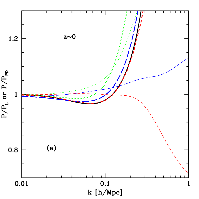
Figure 1: Thick lines show $P(k)/P_{L}(k)$ at $z=0$ for the Peacock and Dodds (PD96) fitting formula Peacock and Dodds (1996) (black, solid), Smith et al. (2003)’s HALOFIT formula (blue, long-dashed), the RG-improved PT of this paper (red, short-dashed), and standard PT (green, dotted). Thin lines show the other cases divided by the prediction of PD96. (a) and (b) are similar except for the axis scales. Note that standard PT was used to calibrate HALOFIT at $k<0.1\,h\,{\rm Mpc}^{-1}$.

Figure 1(a) shows essentially perfect (better than percent level) agreement at $z=0$ between RGPT and the Peacock and Dodds fitting formula Peacock and Dodds (1996) for $k\lesssim 0.3\,h\,{\rm Mpc}^{-1}$. This does not mean that RGPT is perfect – it is likely that the agreement with PD96 is partially a coincidence, because we have no reason to expect their formula itself to be accurate to this level. In fact, because of the approximation discussed above related to decaying modes, RGPT must inevitably have some error as well. I note here that Smith et al. (2003)’s HALOFIT formula is not suitable for testing perturbation theory at low-$k$ because the fit was actually constrained by PT calculations for $k<0.1\,h\,{\rm Mpc}^{-1}$ (R. E. Smith, private communication). The fitting formula is a smooth function, so it is not surprising that it does not agree perfectly with standard PT at $k<0.1\,h\,{\rm Mpc}^{-1}$, i.e., if the PT power is generally greater than the simulation power, the region near $k=0.1\,h\,{\rm Mpc}^{-1}$ will be some average of the two, because a step function is not allowed. It is not surprising that this imperfect fit would be missed by Smith et al. (2003), because the deviation is $<5$%, i.e., smaller than their claimed accuracy. Additionally, the $k<0.1\,h\,{\rm Mpc}^{-1}$ power was not constrained exclusively by PT, because the criterion for using scale free simulation results was different (R. E. Smith, private communication). In any case it is clear that RGPT is an improvement over standard PT.

Figure 1(b) shows the comparison at $z=0$ again, with rescaled axes, this time focusing on higher $k$, including deep in the non-linear regime. I note optimistically that, while the prediction is not precise at high $k$, it continues to be a dramatic improvement over linear theory, i.e., even when the non-linear power is a factor of $\sim 10$ greater than the linear power, the perturbation theory result correctly accounts for most of the difference (admittedly, this was also true of standard PT). If similar improvements are obtained by removing approximations or simply with each additional order of perturbation theory, one could imagine converging quickly to a precise result. However, it is possible, or even likely, that missing higher moments of the velocity distribution will undermine the calculation at high $k$.

One of the notable features of the results is their convergence at high $k$ to the $d\ln P/d\ln k\simeq-1.4$ fixed point of Eq. (14), where the 2nd order PT term vanishes for a pure power law power spectrum (Scoccimarro and Frieman, 1996). At $z=0$ this limit is reached for $k\gtrsim 0.3\,h\,{\rm Mpc}^{-1}$, while at earlier times it is only reached at higher $k$ (e.g., $k\gtrsim 3\,h\,{\rm Mpc}^{-1}$ at $z=3$). Qualitatively, this seems like a positive development. Whatever small-scale structure exists initially, it appears to be effectively taken out of play. This may alleviate one common worry about this kind of PT, that one is integrating over high-$k$ modes that are highly non-linear, violating the premise of the perturbation theory. This fixed-point behavior provides another reason to hope that higher order calculations can significantly extend the range of accuracy of the calculation: it may be that the high $k$ behavior of $P(k)$ can be thought of as a slow rolling with scale, as higher order terms become important, of this kind of fixed-point power law. The fixed point will also be modified by the full inclusion of decaying modes.

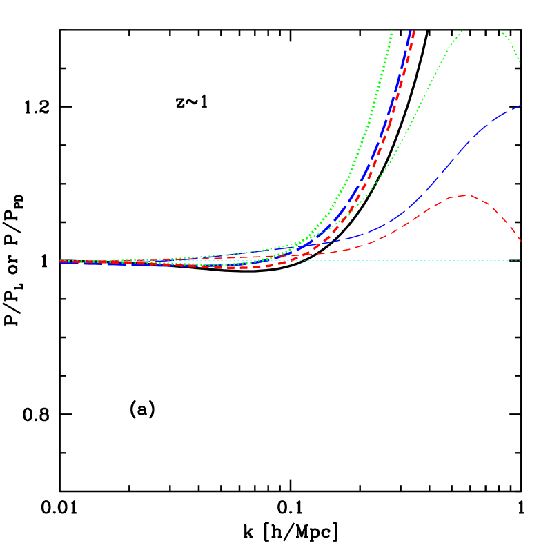
Figure 2: As Fig. 1 except at $z\sim 1$. We label this and subsequent $z>0$ figures by the redshift at which the amplitude of the linear theory power in a flat $\Lambda$CDM model with $\Omega_{m}=0.281$ matches the amplitude in the calculation. The actual redshift in the EdS model used for the calculation is somewhat lower (e.g., for equal $z=0$ linear power, $z=1$ in the realistic $\Lambda$CDM model corresponds to $z=0.61$ in the EdS model).

Figure 2 shows the comparison at $z=1$, a typical redshift for planned galaxy redshift surveys aimed at measuring the baryonic acoustic oscillation feature (Glazebrook et al., 2005). As at $z=0$, RGPT agrees well with the fitting formulas in the mildly non-linear regime, although now the agreement is better with HALOFIT than PD96 at the high $k$ end of this regime. An optimistic interpretation of this figure would be that PD96 is more accurate at low $k$, because it was not constrained by standard PT, but HALOFIT becomes more accurate at higher $k$, as the authors Smith et al. (2003) claim it should be. Dedicated numerical simulations and/or higher order PT calculations testing convergence are needed to determine the true power.

Figure 2b again shows that the RGPT prediction traces the fitting formulas reasonably well deep into the highly non-linear regime. In this case, the agreement is actually as good as the agreement between the two fitting formulas, out to $k\sim 5\,h\,{\rm Mpc}^{-1}$.

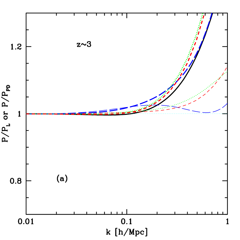
Figure 3: As Fig. 1 except at $z\sim 3$ ($z=2.08$ in the EdS model).

Moving on to $z=3$, relevant to the Ly$\alpha$ forest (McDonald and Miralda-Escudé, 1999; McDonald et al., 2000; McDonald et al., 2006a), and again potentially future galaxy redshift surveys (Glazebrook et al., 2005), we see clear deviation between the PT predictions and the fitting formulas, even in the weakly non-linear regime. This is especially puzzling considering that the RG and standard version of PT actually give very similar predictions in the weakly non-linear regime. This agreement means that the higher order terms that are being effectively re-summed by the RG calculation are not important. Considering the substantial disagreement between the two fitting formulas at very low $k$, I am not ready to conclude that PT is wrong. It may be that the fitting formulas were not well-calibrated in this regime. Focused simulations are needed to test this. Deeper in the non-linear regime at $z=3$, Fig. 3(b) shows that the effect of renormalization becomes substantial, and that RGPT agrees quite well with HALOFIT, while both disagree significantly with PD96. The optimistic reading is that RGPT is very successful, but considering my willingness to dismiss HALOFIT in the weakly non-linear regime, it is probably best to wait for more simulations and/or higher order PT calculations before becoming too pleased with RGPT.

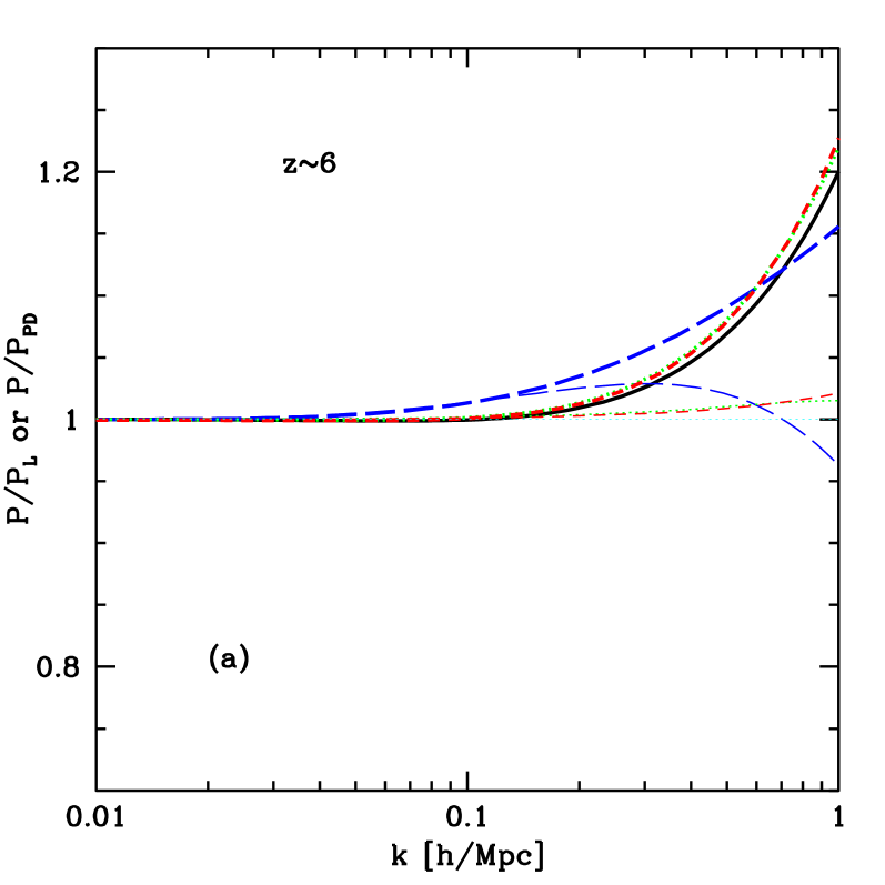
Figure 4: As Fig. 1 except at $z\sim 6$ ($z=4.37$ in the EdS model).

Finally, we consider $z=6$. In the weakly non-linear regime shown in Fig. 4(a), RG and standard PT are essentially identical, and agree quite well with PD96. HALOFIT differs substantially, so again the results are ambiguous. The same can be said for the non-linear regime in Fig. 4(b), where the fitting formulas disagree substantially.

IV Discussion and Speculation

The central result of this paper is Eq. (14), the RG equation for the renormalized power spectrum, demonstrated in Fig. 1(a) to give good results for the power spectrum in the quasi-linear regime at low redshift, where standard PT performs poorly. It is clear from Figs. 1-4 that the RG improvement to standard PT is generally helpful, in both the weakly and strongly non-linear regimes. Except in the most challenging case of $z=0$ and high $k$, the simulation-calibrated fitting formula predictions of Peacock and Dodds Peacock and Dodds (1996) and HALOFIT Smith et al. (2003) are sufficiently contradictory that it is not completely obvious that they are more reliable than RGPT.

It is possible that this method will turn out to be a computational curiosity, maybe leading to improved a posteriori understanding of what we see in simulations, but unable to achieve sufficient accuracy for practical problems, and thus leading to little fundamental change in how we carry out precision cosmology measurements. (It may appear that the method is guaranteed to be useful for describing weakly non-linear galaxy clustering, but this could still be foiled by bias and redshift-space distortions, which I discuss below.) On the other hand, I hope that this line of work is only in its infancy, and will lead to a diversification of computational methods, beyond standard N-body simulations. I am distinguishing here between systematic approximation methods and heuristic ones like the halo model, which rely heavily on calibration by simulations. One of the implicit goals of this work has been to avoid any approximations where the path to improved accuracy is unclear. A good quality for an approximation to have is a clear limit in which it can be expected to return to the exact result. Note that standard simulations are themselves exactly the kind of systematic approximation that I would like to see more of. Simulating a finite volume with a finite number of particles and limited force resolution are all approximations, but each can be tested for convergence as their controlling parameters are changed.

With the hope of stimulating further work, I now discuss a variety of possible directions that could be pursued, although I can’t guarantee that all of these are good ideas:

The first priority should be to include the velocity-velocity and velocity-density power spectra as independent functions to be renormalized, as I discussed extensively in §II.3.2. The main requirement for doing this properly is a straightforward generalization of the standard PT results to allow for general initial conditions, including decaying modes. The $n\simeq-1.4$ fixed-point power spectrum will be modified, hopefully to a more interesting, accurate fixed-point shape.

After that, brute force computation to higher order in perturbation theory should produce more accurate results. The fact that the current calculation is a substantial improvement over linear theory at all $k$ (as opposed to diverging wildly at some point), well beyond the scale where it is no longer very precise, makes me hopeful that each additional order could extend the effective scale significantly. The possibility of estimating the errors in the calculation by comparing results at different orders is an equally strong motivation for going to higher order. [In the same sense, the present calculation should show where linear theory breaks down much more accurately than the common practice of guessing based on the value of $\Delta^{2}(k)=k^{3}P_{L}(k)/2\pi^{2}$.]

These calculations give clear motivation and targets for high accuracy simulation work. RGPT, being a first principles method containing the possibility of internal error control, may in places lead the comparison rather than simply being tested itself. If a higher order of PT is computed, and the results agree between different orders to some level of precision, it is reasonable to expect that the result is correct, independent of simulations. (Missing higher moments of the particle velocity distribution function may be a loophole in this argument, as I discuss below.) With the fixed-point concept in mind, it may be interesting to look more carefully at the evolution of the logarithmic slope of the power spectrum with time and scale in simulations.

Abandoning the first principles philosophy, RGPT results may provide a useful template for a new simulation fitting formula. Because the errors in RGPT are not too large, and should be slowly varying functions of $k$ and cosmological parameters, the new formula could be just a very simple parameterization of corrections to RGPT computed using simulations.

One can obviously apply the techniques of this paper to higher order statistics such as the bispectrum (Gaztañaga and Scoccimarro, 2005; Benabed and Scoccimarro, 2006; Sefusatti et al., 2006), trispectrum, etc. (Ross et al., 2006). As discussed in §II.3.2, one can consider promoting the leading order for these statistics to the more generally possible $\mathcal{O}(\delta_{1}^{3})$ and $\mathcal{O}(\delta_{1}^{4})$ (for the bispectrum and trispectrum, respectively). Bispectrum results can be compared to the simulation fitting formula of Scoccimarro and Couchman (2001). If the trispectrum computation is sufficiently accurate, RGPT should be useful for computing expected statistical errors on the power spectrum, which is notoriously painful to do with simulations (Hamilton et al., 2006). Similarly, errors on higher order statistics may be computable.

Mostly for convenience, I have assumed that the only effect of deviations from Einstein-de Sitter background evolution is to change the linear growth factor. This is probably sufficient in the weakly non-linear regime, but if RGPT is to achieve much accuracy at higher $k$, this assumption inevitably must be relaxed. This is clear, even though the corrections in standard PT are very small, because the dependence of the power spectrum on the equation of state of dark energy, $w$, at fixed observation-time linear theory power (McDonald et al., 2006b), can not be reproduced under the approximation used here. There is simply no way the dependence quantified in McDonald et al. (2006b) can enter the current calculation. Fortunately, even small changes in the right hand side of Eq. (14) can lead to significant changes in the solution of this non-linear equation. It will also be necessary to move beyond the very simple time dependence in Eq. (8) if one wants to include any non-gravitational effects that break this form (e.g., gas pressure).

To describe direct tracers of gas, like the Ly$\alpha$ forest or SZ, gas dynamics could be included in the calculation. Even for weak lensing, which traces mass directly, gas physics has been shown to matter at a level problematic for high precision experiments (Jing et al., 2006). Very rudimentary pressure approximations should be relatively straightforward to include (Gnedin and Hui, 1998). While it may be that very sophisticated implementations of heating and cooling are hopeless, one should remember that there is some non-trivial inclusion of non-linearity in this calculation, so this is at least worth considering.

To describe clustering of galaxies, or other unavoidably inexact tracers of density, some concept of bias will need to be included in the calculation. I think this may be the area where RGPT is most likely to provide a real fundamental improvement over simulations, or at least complement to them. With a large but probably achievable amount of computer power, one can simulate the power spectrum of dark matter and its dependence on a relatively small number of cosmological parameters more or less perfectly. This will not be possible in the foreseeable future for galaxies, so robust, high precision cosmological measurements using them will rely on developing a comprehensive understanding of how relatively microscopic galaxy formation details translate into large-scale clustering patterns. While the separation of scales probably is not clear enough to make the analogy perfect, this is reminiscent of the classic uses of the renormalization group to understand how complex microscopic theories lead to simple macroscopic behavior (Wilson, 1983). The simplest way to introduce bias is to follow Fry and Gaztanaga (1993); Heavens et al. (1998) in writing the galaxy density fluctuation, $\delta_{g}$, as a Taylor series in the mass density, $\delta_{g}=\sum_{i}b_{i}\delta^{i}/i!$, which leads to an expression for the PT power spectrum of galaxies involving a few more terms than the mass power spectrum, but not fundamentally more complicated. This path has been followed by McDonald (2006). Much more ambitiously, one could write local formation rate equations for a galaxy density field and apply perturbation theory to them (something like this was discussed using linear theory in (Tegmark and Peebles, 1998)). For example, $\dot{\rho}_{g}=\rho~{}f(\rho)$, with $\dot{\rho}=-\dot{\rho}_{g}$ to represent depletion of gas, and with both components obeying the usual gravitational evolution equations. The mean galaxy density as a function of time would be an output of the calculation as well as fluctuations. The goal here would not be to write down a realistic local model and compute exact predictions as much as to see what kind of relations between observables can be generically expected. An intriguing possibility is that one could show that, regardless of the small-scale galaxy formation details, bias can only take certain universal forms, described by a small number of free parameters. Note that the validity of the scale-independent bias assumption has never really been proven even in the perfectly linear regime (see Scherrer and Weinberg (1998) for one attempt). This entire discussion of bias of galaxies applies equally well to many other traces of density, e.g., the Ly$\alpha$ forest (McDonald, 2003).

For many applications, redshift space distortions will need to be included. Like bias, these should be relatively straightforward to include in the present RG formulation using the extension of Kaiser (1987)’s linear theory calculation described by Heavens et al. (1998). Scoccimarro (2004) discusses the imperfections of the Kaiser (1987) approach, and proposes alternative ideas which may be useful.

It may be interesting, as a computational curiosity, to see if RGPT can give sensible results for $n\geq-1$ power law initial conditions. In this case the integrals giving the first correction in standard PT truly diverge, in the sense of being infinite rather than just large (Scoccimarro and Frieman, 1996). The integrals can be cut off at wavenumber $k_{c}$, but the results then depend on $k_{c}$, which is arbitrary. One may be able to show that, using the RG as described in this paper, the results will converge as $k_{c}$ is taken to infinity. The small-$A_{\star}$ integration of Eq. (14) will need to be done increasingly carefully as $k_{c}$ is increased, but hopefully convergence to the $n=-1.4$ fixed point will quickly erase all trace of the cutoff. Note that $k_{c}$ could affect the normalization of the asymptotic power law, which would spoil this idea (e.g., it may only work over some limited range of $n$).

One potential limitation in RGPT as presented here is the absence of higher moments of the velocity distribution function, e.g., the dispersion in the velocities of particles around their mean velocity at a point. I wrote the Vlasov equation (2) instead of cutting straight to the hydrodynamic equations to point out this problem, shared by standard PT (subsequently discussed by Afshordi (2006)). Dropping higher moments of the velocity distribution, also known as the single-stream approximation, is not really an added approximation in standard Eulerian perturbation theory. This is surely known to experts (e.g., Buchert and Dominguez (1998)), but may not be universally recognized. One can easily include these moments as variables in the calculation, for example multiplying the Vlasov equation by $p_{i}p_{j}$ and integrating over $p$ gives (after some substitution to remove bulk velocity terms)

$$\frac{\partial\sigma^{ij}}{\partial\tau}+2~{}{\mathcal{H}}~{}\sigma^{ij}+v^{k}~{}\partial_{k}\sigma^{ij}+\sigma^{jk}~{}\partial_{k}v^{i}+\sigma^{ik}~{}\partial_{k}v^{j}+\frac{\partial_{k}\left[\left(1+\delta\right)q^{ijk}\right]}{1+\delta}=0~{},$$ (28)

where $\partial_{k}=\partial/\partial x^{k}$, $\sigma^{ij}(\mathbf{x},\tau)\equiv\left<\delta v^{i}~{}\delta v^{j}\right>$, $q^{ijk}(\mathbf{x},\tau)\equiv\left<\delta v^{i}~{}\delta v^{j}~{}\delta v^{k}\right>$, with $\delta v^{i}$ the deviation of a particle’s velocity from the local mean velocity (note that a $\sigma^{ij}$ term would appear in Eq. 6 if I had not dropped it). Unfortunately, the lowest order evolution equations contain only the Hubble drag term, so any initial velocity dispersion will self-consistently disappear from the perturbation theory. Furthermore, higher order equations contain no source terms, meaning that if the velocity dispersion is initially zero it can never become non-zero. In fact, Valageas (2001) showed that even perturbation theory using the distribution function directly leads to the same result. This is a vexing problem because stream crossing is clearly ubiquitous in the real Universe; however, Scoccimarro (2001) estimated that it only becomes significant at $k\gtrsim 1\,h\,{\rm Mpc}^{-1}$, so it may not be fatal for intermediate scales. It seems likely that, if these variables really matter, there should be some way to recover them using a RG method. The basic idea is that, no matter how small the effect is in the bare perturbation theory, if it is dynamically relevant it will grow through a RG equation like Eq. (14). Note that even WIMP cold dark matter has a very small seed velocity dispersion (Green et al., 2004). The solution is probably to simply retain the dispersion variable in the calculation, even though it is decaying, in the same way I have argued above that one should retain the decaying combination of $\delta$ and $\theta$ – because it can be rapidly fed by higher order terms. Vorticity, $\mathbf{\nabla}\times\mathbf{v}$, falls out of the standard PT calculation for the same reason velocity dispersion does (Bernardeau et al., 2002). The standard calculation makes use only of the velocity divergence, $\mathbf{\nabla}\cdot\mathbf{v}$. A method that successfully reintroduces velocity dispersion may also work for vorticity.

I started this line of work with the intention of using a significantly different type of renormalization group method, based on integrating out (averaging over) small-scale (high-$k$) modes while modifying the equations describing evolution of the large-scale modes in a way that preserves their statistics (Shankar, 1994). This method usually starts with a path integral formulation of the problem. Valageas (2001) presented a path integral approach to large-scale structure using the full distribution function, and it should not be too hard to write something similar for the usual moments of the distribution function. Velocity dispersion should arise inevitably in this approach, because smoothing a dispersionless field obviously produces dispersion. It is less inevitable that this dispersion will actually fundamentally change the outcome of the calculation, because the effect of these velocities is already present in the standard PT calculation. Among other possibly interesting features, the noise discussed in previous RG approaches to large scale structure (Barbero G. et al., 1997; Domínguez et al., 1999) may be generated naturally using this approach (i.e., if high-$k$ modes are eliminated, the time evolution of the remaining modes will no longer be perfectly deterministic).

Further work could elucidate the connection between this work and the re-summation method of Crocce and Scoccimarro (2006a, b). Related renormalization group procedures, starting from general relativistic perturbation theory, are used by Nambu (2000) and Kolb et al. (2005) to compute the back-reaction of inhomogeneities on the global evolution of the Universe.

Finally, the success of the RGPT calculation in this paper, which leads to what looks like a time evolution equation for the power spectrum, suggests that it might be useful to consider the exact time evolution equation for the power spectrum, $\dot{P}(k)\propto 2~{}{\rm Re}\left<\dot{\delta}_{\mathbf{k}}~{}\delta_{-\mathbf{k}}\right>$, where $\dot{\delta}_{\mathbf{k}}$ is obtained from the usual evolution equations. The usual argument against this would be that $\left<\dot{\delta}_{\mathbf{k}}~{}\delta_{-\mathbf{k}}\right>$ involves higher order terms like the bispectrum, which then require their own time evolution equations, and so on, leading to an infinite hierarchy of equations. Firstly, this could be a useful way to look at perturbation theory, especially if we are going to be renormalizing statistics like the power spectrum instead of the field itself. Second, one may be able to make progress by simply solving these equations numerically, in the same sense that simulations are usually used. One could, for example, truncate the hierarchy by replacing the connected spectra at some level by the appropriate functions of lower order spectra given by perturbation theory, and look for convergence in the results as higher order terms are added. The advantage of working with statistics of the density field rather than the density field itself is enormous. One obtains the desired results directly rather than averaging over fluctuations in simulations, where there is usually an unavoidable conflict between the need for large boxes to limit finite volume effects like sample variance, and the need for high force and mass resolution to properly compute small-scale structure. The fact that we are working with continuous, relatively slowing varying functions, rather than wildly fluctuating fields, allows many fewer points to be computed, e.g., we can compute a power spectrum over many decades of dynamical range by interpolating between a few tens of logarithmically spaced computation points when millions or billions of particles would be needed to cover the same range with a simulation. Tasks that at first glance seem arduous, e.g., parameterizing the trispectrum or even higher spectra and setting up their evolution equations, should be considered in contrast to the decades of person-power expended on simulations.