Distances to Anomalous X-ray Pulsars using Red Clump Stars

Abstract

We identify “red clump stars” – core helium-burning giants – among 2MASS stars and use them to measure the run of reddening with distance in the direction of each of the Galactic Anomalous X-ray Pulsars (AXP). We combine this with extinction estimates from X-ray spectroscopy to infer distances and find that the locations of all AXP are consistent with being in Galactic spiral arms. We also find that the 2–10 keV luminosities implied by our distances are remarkably similar for all AXP, being all around $\sim\!1.3\times 10^{35}{\rm\,erg\,s^{-1}}$. Furthermore, using our distances to estimate effective black-body emitting radii, we find that the radii are tightly anti-correlated with pulsed fraction, and somewhat less tightly anti-correlated with black-body temperature. We find no obvious relationship of any property with the dipole magnetic field strength inferred from the spin-down rate.

1 Introduction

The Anomalous X-ray Pulsars (AXPs) are young, energetic, X-ray bright isolated neutron stars, with spin periods of the order 10 s. They are called anomalous since their luminosity far exceeds the energy available from spin-down, and no binary companions are seen. AXPs (along with the related Soft Gamma-ray Repeaters or SGRs) are now believed to be magnetars (Thompson & Duncan, 1996). Magnetars have huge external magnetic fields ($\sim 10^{14}$G) and even larger internal fields. It is the decay of the magnetic flux which provides the luminosity seen, and is responsible for a whole array of observational effects such as bursting and giant flares. See Woods & Thompson (2004) for a summary of recent observational data on magnetars, and how they are modeled.

Since they are young remnants of massive, short-lived progenitors, all of the AXPs are found in the Galactic plane (except for CXOU J010043.1$-$721134 which is in the Small Magallanic Cloud). This causes a major obstacle to observations: high interstellar extinction, manifested as photo-electric edges from different elements in the soft X-ray band, and as continuum extinction from dust in the optical and near-infrared. Since the amount of extinction has been difficult to estimate accurately, the spectral energy distributions of AXP have been subject to large uncertainties (Hulleman et al. 2004; Durant & van Kerkwijk 2005, 2006).

Furthermore, even if the interstellar absorption is well-characterized, distances and therefore absolute fluxes are difficult to determine. The simplest distance estimate is made by requiring that the black-body component typically inferred from the X-ray spectrum arises from a neutron-star sized area. We do not, however, expect the surfaces of AXPs to be homogeneous, both on observational grounds (they pulsate) and from theoretical considerations (the magnetic field, which affects the heat conduction, will vary across the surface).

For AXPs that are associated with supernova remnants or other interstellar structure, a more direct distance estimate can be made using 21 cm H I measurements and the Galactic rotation curve. Convincing cases for associations with supernova remnants have been made for two AXPs: 1E 2259+589 with CTB 109 (Gregory & Fahlman, 1980), and 1E 1841$-$045 with Kes 73 (Sanbonmatsu & Helfand 1992). Furthermore, Gaensler et al. (2005) found an H I bubble coincident with the direction of AXP 1E 1048.1$-$5937, which they suggest was created by the winds of the massive progenitor of the AXP (see Muno et al. 2006 for a discussion of possible massive progenitors to AXPs). Even for these systems, however, distance estimates can be rather uncertain, with different authors finding inconsistent results (we discuss this further in §4 and 5).

For sources in the Galactic plane, a different clue to the distance is available if one has a good measure of the interstellar extinction, and the run of extinction with distance can be determined independently. This works because the extinction increases with distance, more so towards star-forming regions and molecular clouds.

The so-called red clump method provides a means for deriving the function of reddening versus distance in any given line of sight, based on field stars over a relatively small area. López-Corredoira et al. (2002) noted that in an infrared color-magnitude diagramme of a stellar cluster ($J-K$ versus $K$ for example), core helium-burning giants, or red clump stars, form a well-defined and easily-identified concentration of stars redward of the main sequence. Stars spend up to 10% of their lifetime in this phase, and are much more luminous than typical main sequence stars. Because their helium cores all have roughly the same mass, their luminosities are largely independent of the total stellar mass. Furthermore, their infrared colours are insensitive to metallicity. As a result, they are good infrared standard candles and if the red clump can be identified at each of a range of distances, then the reddening at each distance can be calculated. The method has been used not only by Lopez-Corredoira et al. (2002) to measure the density distribution of stars in the Galaxy, but also by, e.g., Drimmel et al. (2003) to map the distribution of dust.

Here, we apply the red-clump method to measure distances to the Anomalous X-ray Pulsars. In section §2, we first describe how we applied the red-clump method, focussing on the AXP for which the method was most tricky, and in section §3 we use this field to test the reliability of the method, and to estimate uncertainties in the derived values. In §4, we present the results of the red clump method applied to each of the Galactic AXPs, and we discuss the implications in terms of distance. In §5, we compare our new distances with those in the literature, in particular for the controversial case of 1E 2259+589 and the associated supernova remnant CTB 109. In §6, we use our results to infer luminosities and emitting radii, and discuss how these depend on other AXP properties. We draw conclusions in §7.

2 Method

Our method closely follows that described by López-Corredoira et al. (2002). We start with data from the 2MASS catalog (Skrutskie et al., 2006) in the J- and K_S-bands. (From here on, we refer to the K_S band as K for brevity.) Since all the Galactic AXPs lie along the plane, we find a large number of 2MASS stars at relatively small radii around each source. For the analysis, we initially chose the 9999 nearest stars and used these to construct $J-K$ versus $K$ color-magnitude diagrammes (covering circular fields around each AXP with radii in the range 9$\farcm$6 to 20.6$\farcm$). Below, we first discuss in some detail the results for the AXP 1E 1048.1$-$5937, for which applying the method proved to be most tricky.

Figure 1 shows the colour-magnitude diagramme for 1E 1048.1$-$5937. On this graph, reddening alone causes stars to move to the right and slightly down (redder and fainter) and increased distance alone causes stars to move down (fainter in all bands). From the Figure, one sees that the main sequence (on the left of the diagramme) contains the bulk of the stars. Due to the large range in intrinsic luminosities, stars from different distances and reddenings show up as an amorphous conglomeration, with an increasing range in color towards the faint end. The red clump, however, shows up as a clearly defined stripe (center), representing stars of the same luminosity and color at different distances and reddenings. Since red-clump stars are relatively rare, few are found at magnitudes brighter than about $K=9$ (distance $\lesssim\!1.3\,$kpc). Stars redward of the red clump are either poorly measured (e.g., blended in the K band), background super-giants or young stars with infrared excess.

One can select any range in $K$ in the diagramme in order to find the peak of the red-clump star distribution for that range. Our method works by identifying this peak for various ranges in K-band magnitude. As an example, we have selected a 0.6 mag-wide strip around $K=12.9$ for analysis. The histogram of $J-K$ colors for the selected stars is shown in Fig. 2. To find the peak of the red-clump distribution, we fit a Gaussian function to the histogram values. The main complication is contamination by background, highly reddened main sequence stars (see again Fig. 1). These tend to skew the distribution, and for $K$ approaching 14 overwhelm the Gaussian feature. To account for these contaminants, we fit the histogram with a power law plus Gaussian:

$$y=A_{\rm cont}(J-K)^{\alpha}+A_{\rm RC}\exp\left(-\frac{1}{2}\left[\frac{((J-K)-(J-K)_{\rm peak})^{2}}{\sigma^{2}}\right]\right)$$ (1)

where $(J-K)$ is the stellar color, $(J-K)_{\rm peak}$ is the peak of the distribution, $\sigma$ the width of the peak, $A_{\rm RC}$ and $A_{\rm cont}$ the normalizations of the red-clump and contaminant terms, and $\alpha$ the power-law index.

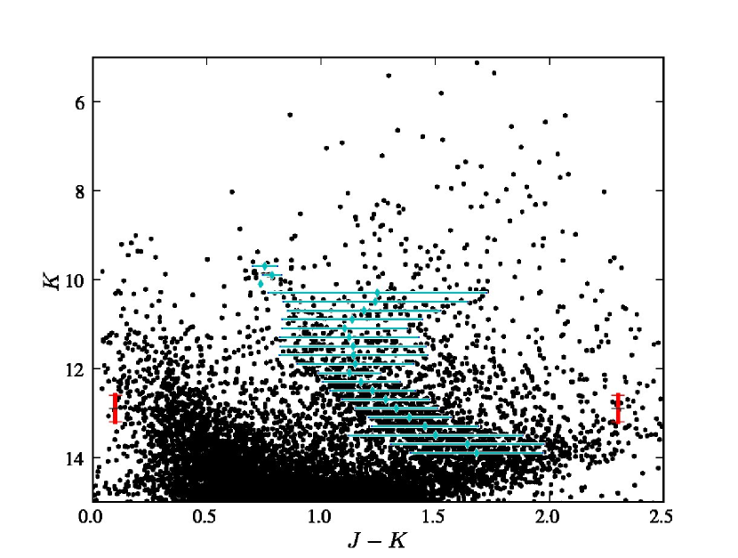
Figure 1: Color-magnitude diagram for 9999 stars within 11$\farcm$4 of 1E 1048.1$-$5937. Main-sequence stars are found from about $(J-K,K)=(0.2,10)$ to (0.5,14), and red-clump stars show up as an over-density from about (1.0,10) to (1.7,14). The fitted location of the red-clump peak (diamonds) and its extent (bars, showing $\pm 1\sigma$ or roughly the full width at half maximum) are marked. The error bars (left and right edges) show the location and size of the strip used to create the histogram shown in Fig. 2. The poor fits near $K=11$ are discussed in §3.

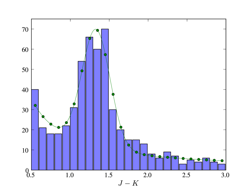
Figure 2: Histogram of the $J-K$ values of stars extracted from Fig. 1 in a 0.6 mag interval around $K=12.9$. Overdrawn is a fit to this histogram using Eq. 1, with the curve showing the analytical function and the points the best-fit values.

Equation 1 is fitted using a standard least-squares algorithm, assuming the errors in each histogram bin are the same. This process is repeated for successive bins in $K$ until the 2MASS completeness limit is reached. Figure 1 shows the fitted red clump positions overdrawn on the color-magnitude diagramme. Features from this plot, such as the poor fits around $K=11$, will be discussed in the next section.

Since our algorithm finds only local minima in the $\chi^{2}$ surface, it is necessary to supply reasonable starting values to the routine. We found that if we chose our strips in $K$ to overlap, and used the best-fit values of the previous histogram, smooth changes in the peak were well followed. To increase robustness, our algorithm also checks the relative residuals of fits performed with a few different initial values of $(J-K)_{\rm peak}$; this covers the case where there is a sudden jump in reddening. Note that the choice of the range in $K$ of each histogram and the extent to which these strips overlap is arbitrary, but should not change the results. We test this below.

Assuming the intrinsic color $(J-K)_{0}=0.75$ and the intrinsic luminosity $M_{K}=-1.65$ (Wainscoat & Cowie 1992), the translation of $J-K$ versus $K$ into reddening versus distance corresponds to decomposing the reddening and distance vectors on the diagramme for each red-clump peak found. The infrared color excess can be expressed as a visual reddening through (e.g., Schlegel et al. 1998):

$$A_{V}=\frac{(J-K)_{\rm peak}-(J-K)_{0}}{0.164}$$ (2)

The distance is then (correcting for reddening in K):

$$d=10^{0.2(K-M_{K}-0.112A_{V})}\times 10\,\rm{pc}.$$ (3)

3 Robustness and Uncertainties

The approach discussed above for converting a 2MASS dataset into a run of reddening with distance does not yet yield estimates of the uncertainties. Here, we investigate the error analysis for the field of 1E 1048.1$-$4937 in detail. We chose this field since it exemplifies the problems faced, and lies near one of the most complicated regions of the Galaxy, the Carina Complex. None of the other five AXP fields are more complex.

For our discussion, we estimate the formal uncertainties on the location of the red-clump peak with $\sigma/\sqrt{N_{\rm RC}}$ (where the number of red-clump stars $N_{\rm RC}=\sqrt{\pi}\sigma A_{\rm RC}$, with $\sigma$ and $A_{\rm RC}$ from Eq. 1), which should be a good approximation if the Gaussian is a reasonable fit for the distribution of infrared colors in the red clump, and if the contamination by other stars is not too large. For the test field, the FWHM of the peak is typically $\approx 0.3$ mag and the number of stars of order 100s, giving uncertainties of the position of the peak $\sim 0.02$ mag (one-sigma).

In principle, one could derive better formal uncertainties, e.g., by calculating the $\chi^{2}$ values around the best-fit function, or – more appropriately for a counting problem with Poissonian statistics – using a maximum-likelihood method (which might even take into account the probability distributions in $J$ and $K$ for each star). We believe, however, that a better approach is to keep the estimate of the formal errors simple and combine it with empirical tests for systematic effects using different subsets of stars and using multiple fields.

The first test we did was to try different cuts on the 2MASS data using the magnitude error estimates and photometric quality flags, in order to keep only the best measured points. We found, however, that this had the sole effect of truncating the CMD at brighter magnitudes, without significantly tightening the spread in the red-clump stars at any magnitude. This suggests that any spread in the red-clump stripe on a CMD beyond the typical measurement error is due predominantly to field inhomogeneities. Thus, in order to find the reddening to as large a distance as possible, we continue to use all the available 2MASS stars in a given field.

An important feature that can be seen for the bins between $K=10.5$ and 11.5 in Fig. 1 is that there seems to be overdensities at both $J-K=0.9$ and $J-K=1.2$ and that the fitted points lie in between these two. This suggests that the reddening at these distances is variable across the field. Since two peaks are visible, part of the field might be obscured by denser interstellar matter.

To investigate the inhomogeneity in reddening, and to determine how this affects the sensitivity of method, we analyzed six fields at a distance of 15′ from 1E 1048.1$-$5937 (note that these fields overlap somewhat with the target field). Figure 3 shows the resulting graphs of $J-K$ versus $K$ (we show this graph rather than $A_{V}$ versus $d$, since $d$ depends on both values). One sees that the distribution of reddenings is trimodal, with fields 1 and 6 showing consistently less reddening as a function of distance than fields 2, 3 and 5, but merging to the same value for faint $K$ (note that some fields appear to show a decrease in reddening; this is due to the same bimodality that affects the central pointing). Field 4 shows consistently higher reddening, and is the line of sight passing towards the cluster to the west. Thus, there is structure in the Galactic dust distribution: a dust cloud appears to cover the field gradually from the North-West with increasing distance. Considering the complex structure of the local Carina Nebula, this is not surprising; it is simply a consequence of the large reddening gradients in the area.

From Fig. 3, comparing fields with similar runs of $J-K$ as a function of $K$ (such as 1 and 6, and 2 and 3), one sees that the uncertainties inferred from the Gaussian fit (which are similar for all fields) agree roughly with the scatter between those fields, suggesting that they are reasonable estimates of the uncertainties. (One also sees that compared to the scatter along the curve, the error bars appear to be overestimates – this, however, is a consequence of the fact that the points are not independent, as the strips in $K$ overlap.)

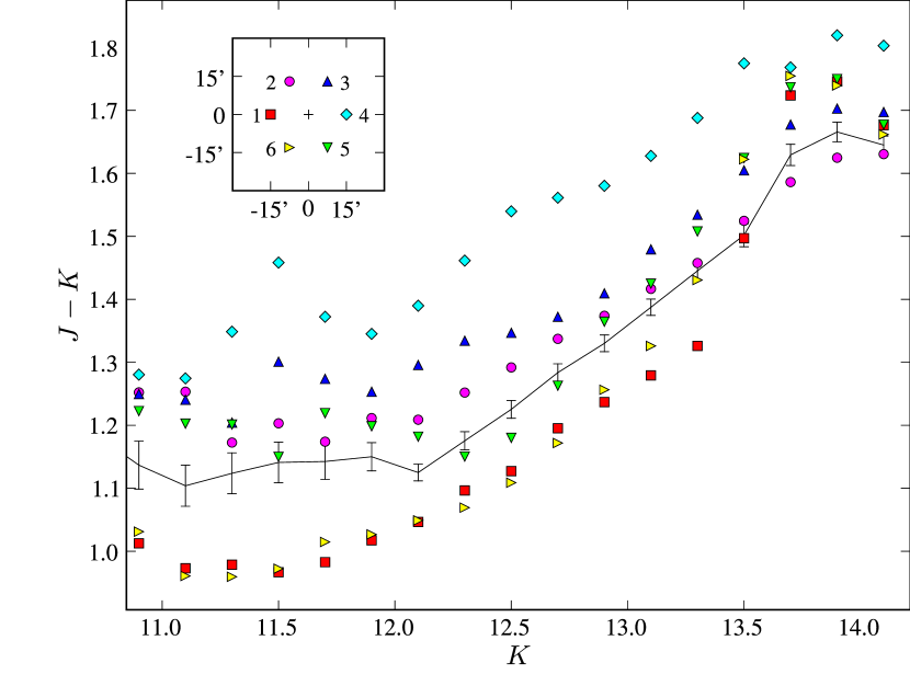
Figure 3: Color of the red-clump stars as a function of magnitude for the field around 1E 1048.1$-$5937 (curve with error bars) and six fields surrounding it (symbols). Field 1 is offset by 15′ to the East, and the other fields are placed anti-clockwise with increasing number (see inset).

Given the inhomogeneity in reddening, we checked whether chosing a smaller field would yield a tighter fit. Figure 4 shows a comparison of the results for the original set of 9999 stars around 1E 1048.1$-$5937 with the results for just the central one-third of those stars, as well as, for comparison, for a randomly chosen one-third of the stars. Interesting behavior is seen in the randomly-chosen curve: generally it follows the curve of the original sample (with increased error bars), but around $K=12$ the inferred $(J-K)$ color decreases a little and is lower than inferred from the original sample. This is due to the competition between the two areas with different reddening in the field. With fewer stars, the fit is more liable to jump from one over-density to the other. For the central sub-sample, however, this does not occur. Instead, it shows consistently lower reddening than the original sample at all values of $K$. The errors are only slightly larger, since the smaller number of stars is offset by the smaller spread in the colors of the red-clump stars.

From our tests, we conclude that in the field of 1E 1048.1$-$5937 a dark cloud towards the North obscures some fraction of area within the 11$\farcm$4 radius covered by the original 9999 stars, but it does not cover the source and hence should be ignored in determining the run of reddening with distance.

More generally, we conclude that, since our aim is not to determine accurately the average reddening in the field, but rather to find the reddening at the center of the field only, we should use the minimum number of stars required for our method to work reliably. Empirically, we find that this is $\sim\!3000$ stars; with fewer stars, the red-clump peak becomes poorly defined due to small-number statistics.

In the case that there remains substantial inhomogeneity within the small field under examination (this is certainly possible, but it turns out not the case for the AXP fields), we must raise an important caveat to the use of the method. Because the over-desity finding rutine picks the best Gaussian feature out of the color histograms, it will be biased towards the more homogenous part of the field. If the field is highly inhomogenous, it may not be able to locate the red-clump satisfactoraly; if a compact dense cloud obscures part of the field, then the method will give the reddening of the unobscured part of the field, since the cloud will have strong column density gradients across it.

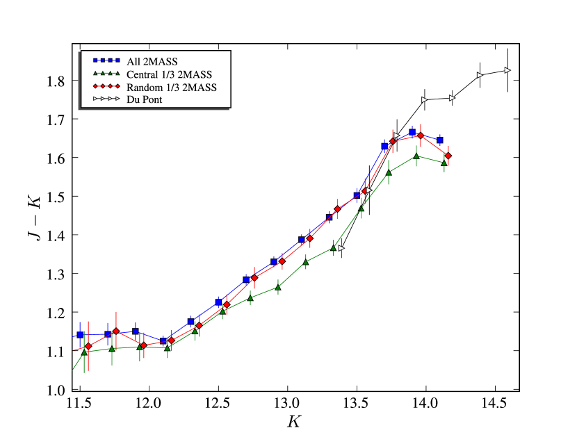
Figure 4: Color of the red-clump stars versus magnitude in the direction of 1E 1048.1$-$5937 for different subsamples (see inset). The curves have been slightly offset in $K$ for clarity.

The next effect we checked is that of the choice of the size and overlap of the bins in $K$. In order to have as high a distance resolution as possible, one would like to use bins in $K$ that are as small as possible. In order for the red-clump peak to be better defined on each histogram, however, one would prefer more stars and a narrower distribution of red-clump star colors. As discussed above, increasing the field size in order to use more stars does not help since the reddening may be non-uniform. The same is true for increasing the K-bin sizes: different colors from different distances will tend to blur the red-clump peak. Since in this case this also comes at the cost of reduced distance resolution, we opt for bin sizes as small as possible which still give reliable results: 0.6 mag, with steps of 0.2 mag. The overlap factor does not change the results or our method, but it is convenient computationally and also allows us to determine slightly more accurately the locations of jumps in reddening.

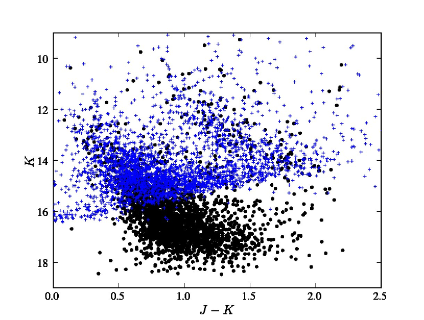
Figure 5: Deeper color-magnitude diagram of the field of 1E 1048.1$-$5937, from Du Pont imaging. The Du Pont sources are shown as black circles, and the 2MASS points (from the closest 3300 stars) as crosses.

The final thing we checked is the effect of the 2MASS limiting magnitudes on our measurements. Our precise estimate of the distance of 1E 1048.1$-$5937 from 2MASS data alone is uncertain, because the last point in our graph of $J-K$ versus $K$ is likely affected by the incompleteness to fainter and to redder sources. To check for this, we obtained further, deeper JK infrared imaging data from the Wide-field Infrared Camera on the Du Pont 2.5 m telescope, Las Campanas (see Persson et al. 2002). We subtracted a sky frame from each image using the median of the science frames (this is required because of an additive component to the noise from fringing), registered and stacked the images. We tied the photometry directly to 2MASS using many stars cross-identified on each of the chips.

Figure 5 shows the new, deeper color-magnitude diagram for stars in the field of 1E 1048.1$-$5937. This includes stars from the chip containing the AXP and two adjacent chips (each chip has a size 200″ square). One sees that down to $K=13$, $J-K=1.4$, which corresponds to the last reliable red-clump location from the 2MASS data, the Du Pont and 2MASS data are consistent, having overdensities at the same colour. However, for the next group, at $K=14$, $J-K=1.8$, the Du Pont data indicate a location redder than the 2MASS data would have suggested. Thus we conclude that the reddening rises more quickly in this region, and the AXP is closer than otherwise would have seemed. We show the $J-K$ values obtained from the Du Pont data in Figure 4 and use these for the final point on the reddening curve for 1E 1048.1$-$5937 in Figure 7.

As mentioned above, the challenges faced in the field of 1E 1048.1$-$5937 are more severe than those for any of the other fields; none show reddening gradients as large, and for all the other sources (except 1E 2259+586, see §4) the appropriate value of the color excess lies either well before or beyond the completeness limit. Using what we have learned here, we perform our analysis on the central 3300 stars near each AXP, and infer uncertainties using the simple estimate from counting statistics.

4 Results

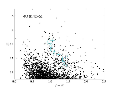
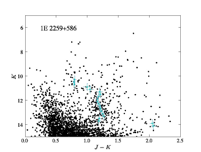
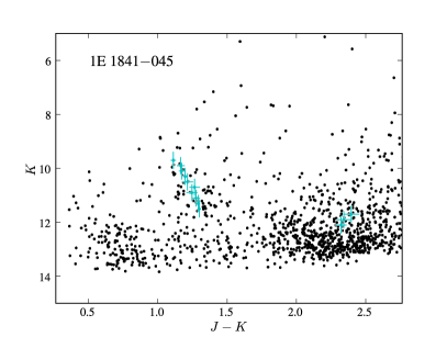
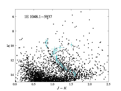
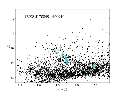
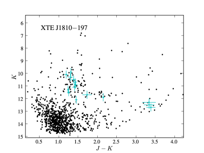
Figure 6: The color-magnitude diagrams used to infer the location of the red clump as a function of brightness, derived from the nearest 3300 2MASS stars around each object (within 5 to 12′). Overdrawn are the fitted red-clump peak colors together with the 1-$\sigma$ uncertainties.

We determined the color of the red clump as a function of brightness using the nearest 3300 stars for each of the six Galactic AXP. In Table 1, we list the size of the field covered by these stars, and in Fig. 6 we show the corresponding color-magnitude diagrams, with the fitted locations of the red-clump stars indicated.

In converting our results to reddening as a function of distance, we prefer to use non-overlapping points. In choosing the points to use, however, one has a certain freedom to pick those that have with the smallest errors, and that show features the clearest. We attempt to do this, and check against the original color-magnitude diagrammes that the breaks occur at the correct values of $K$. In interpreting the fitted points, we also use the fact that reddening can only increase with distance (e.g., we reject a poorly measured point with high reddening in favor of a later, better measured point with lower reddening).

Figure 7 shows the resulting runs of reddening with distance, with associated uncertainties. With X-ray extinction estimates for the AXPs, distances can simply be read off the graphs by first converting to $A_{V}$ using $A_{V}=N_{H}\times 5.6\times 10^{-22}$ cm² (Predehl & Schmitt, 1995). For three of the AXPs – 4U 0142+61, 1E 2259+589 and 1RXS J170849.0$-$400910 – new, model-independent estimates of the extinction were found by Durant & van Kerkwijk (2006) using photo-electric absorption edges in high-resolution X-ray spectra. These are listed in Table 1; the uncertainties reflect the accuracy with which the depths of the various features could be measured. For one further AXP, 1E 1048.1$-$5937, our measurement was not very constraining, while for the remaining two, 1E 1841$-$045 and XTE J1810$-$197, no suitable high-resolution X-ray spectra were available. Hence, for these three AXPs, we use the extinction estimates compiled in Woods & Thompson (2004). These estimates are based on broad-band fits to the X-ray spectra, which means that their accuracy depends on the adequacy of the model (typically a two-component model composed of a power law and a black body). From a comparison of similar estimates with our direct measurements for the three AXPs, we expect that, at the relatively high extinctions found for these two sources, the estimates should be accurate to about 10%.

Before continuing, we should address a possible worry: that a large uncertainty is introduced in the various conversions used. First, above we implicity converted photo-electric absorption edges by metals to an equivalent hydrogen column $N_{H}$, and that in turn to visual extinction $A_{V}$. This is not as uncertain as it appears, however, since the relation of Predehl & Schmitt (1995) between X-ray and visual extinction, while quoted in terms of hydrogen column $N_{H}$, was based on X-ray measurements that were sensitive to metals along the line of sight, not hydrogen, just like ours. Hence, there is no uncertainty associated with, e.g., the metallicity or the hydrogen to dust ratio. A second worry one might have is about selective extinction, i.e., variations in the interstellar extinction law (usually parametrised by $R_{V}\equiv A_{V}/E_{B-V}$). There is, however, far less variation in the infrared (e.g., Mathis 1990). Since the optical extinction estimates of Predehl & Schmitt were largely based on a standard extinction law, we should thus circumvent any problems at visual wavelengths by using the same standard relation between infrared and visual extinction. (Indeed, it might well be that one would find a tighter relation than that of Predehl & Schmitt (2005) if one redid the analysis in terms of infrared extinction.)

From Fig. 7, one sees that for most sources, the measured reddening places the source at a jump in the run of reddening with distance. As a result, the uncertainty in the distance estimate is dominated not by uncertainty in $A_{V}$, but by the accuracy with which the jump can be located, which in turn is determined by the size of the bins in $K$. A bin size of 0.6 mag corresponds to a 15% uncertainty in distance. (As discussed above, the size of the bins was chosen to give the best distance resolution yet yield reliable measures of reddening without using a large field and thus increasing the risk of bias by spatial variations in reddening.) The only source not located at a jump in reddening is 1E 1048.1$-$5937. Hence for this source, uncertainty in the distance is dominated by the (relatively large) uncertainty in the reddening estimate.

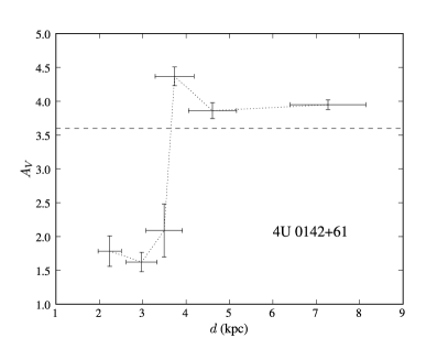
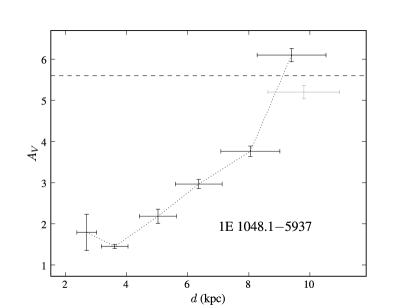
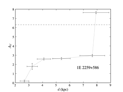
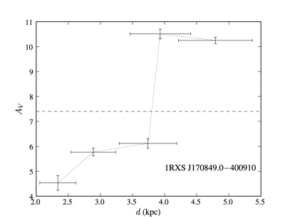
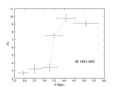
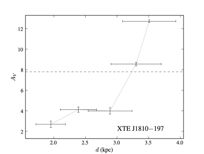
Figure 7: Run of reddening with distance along the line of sight to the six Galactic AXPs. The best estimate for the reddening for each object is shown by a dashed horizontal line (for uncertainties, see Table 1 and the text); note that the estimated $A_{V}=14$ for 1E 1841$-$045 falls outside the graph. The grey point in the graph for 1E 1048.1$-$5937 is discussed in the text.

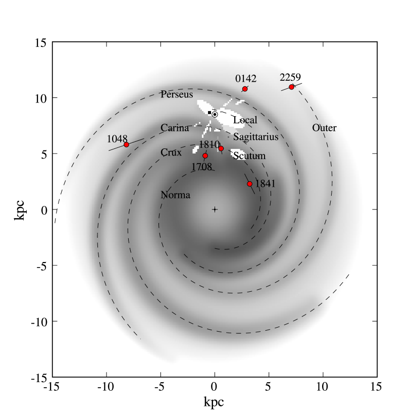
Figure 8: Schematic map showing the positions of the AXPs in the Galactic Plane relative to the Galaxy’s spiral arms. The AXPs are indicated with circles and labeled with abbreviated names, the Galactic center is marked with a “$+$” sign, and the location of the sun with a $\odot$ symbol (at a galactocentric distance of 8.5 kpc). Spiral arms are shown using a fit with a simple four-arm logarithmic spiral model (dashed lines, see Cordes & Lazio, 2002) and free electron density (grey scale, taken from Cordes & Lazio, 2002). The white patches are local interstellar cavities and the dark spot near the sun is the Gum Nebula. The grey scale backdrop has been rescaled to fit these axes.

Table 1 gives final inferred distances and limits. Below, we describe the results for each object in more detail, trying to match rapid increases in reddening with known spiral arms, and locating the AXPs in the Galaxy (see Fig. 8). This can be viewed as an update of the similar map shown in Gotthelf & Vasisht (1998; their Figure 4). We focus on the outcome of our analysis, deferring a more detailed comparison of the implied distances with previous determinations to §5, and a discussion of the implications in terms of luminosities and other derived quantities to §6.

4U 0142+61.

In this field, two regions of reddening are seen, $A_{V}\simeq 2$ in the near field and $A_{V}\simeq 4$ out to large distances. The latter confirms the statement by Hulleman et al. (2004) that the reddening could not exceed $A_{V}\simeq 5$ in this direction, based on the colors of a background galaxy and of field stars. From the estimated reddening to the source of $A_{V}=3.6\pm 0.2$, we conclude that the AXP is located in a region of rapidly rising reddening at $d\simeq 3.5\,$kpc. Likely, this region is associated with the Perseus arm.

Looking in more detail at Fig. 6, one sees that for $K>13.5$, one can no longer identify the over-density of red-clump stars. The stripe seen at lower $K$ does not continue and no over-density is seen redward of this stripe either, as could be caused by a sudden increase in reddening. Most likely, this indicates simply that there are not many red-clump stars beyond a distance of $\sim\!8\,$kpc. Consistent with this, one sees that the red side of the main sequence has a smooth distribution as $K$ increases from 13 to 15; if the absence of red-clump stars beyond $K>13.5$ were due to a large, sharp increase in reddening, this should be visible for the main-sequence stars too.

1E 1048.1$-$5937.

Reddening rises continuously in this field, almost linearly with distance out to $\sim\!12\,$kpc. This is probably due to the Carina Arm, which lies along the line of sight in this direction (Dame at al. 2001; Fig. 8). Our estimate of the reddening to the AXP places it at the tail end of this function. The 2MASS completeness limit in the J-band causes the stars to go undetected beyond a line $((J-K),K)=(1.5,15)$ to (2.5,12). Our distance estimate is therefore based on the Du Pont photometry we obtained, which goes deeper than the 2MASS survey (see §3 and Figure 5). This affects only the last point in the graph of $A_{V}(d)$. We include in Figure 7 the furthest point which would have been obtained from the 2MASS data alone in faint grey.

Despite the existance of a new estimate of reddening from Durant & van Kerkwijk (2006), the value given was not very constraining. We therefore have used the old estimate base on fitting the sum of a black-body and power-law to the X-ray spectrum. In this particular case, that approach should be the least error prone, since the power-law component is the shallowest of the AXPs, and hence has relatively little influence on the low-energy region of the spectrum, to which $N_{H}$ is most sensative (Woods & Thompson, 2004).

Our estimated distance is around 8.6 kpc. This distance estimate is inconsistent with that of Gaensler at al. (2005); we return to this in §5.

1E 2259+589.

In this field, the reddening is low up to $d\simeq 3\,$kpc, next rises to $A_{V}\simeq 3$, and then stays at that value out to about 6.5 kpc, where it shows a second and larger jump. From Fig. 6, one sees that this second region of reddening is inferred from only a few stars at around $J-K=2.0$ and $K=14$. We believe it is genuine, however, for several reasons. First, at $K=14$ there is a notable absence of stars at $J-K=1.2$, below the location of the stripe for brighter magnitudes. Second, in contrast to what we saw for 4U 0142+61 above, the main sequence’s red edge does appear to show a jump, from about $J-K=0.7$ at $K=13.5$ to $J-K=1.2$ at $K=14$. Third, the two jumps have a nice correspondance with expected jumps due to spiral arms, with the nearer one being due to the Perseus arm and the farther one due to the Outer arm (Fig. 8).

Assuming the second jump in reddening is real, the AXP’s estimated reddening of $A_{V}=6.3\pm 0.7$ places it into this region, and thus likely in the Outer arm, at $d\simeq 7.5\,$kpc. Were the last point in the curve of $A_{V}(d)$ affected by incompleteness of the 2MASS sample, as was the case for 1E 1048.1$-$5937 (above), this would move the point even further redward, make the jump steeper, and not significantly affect the estimated distance. In §5, we compare this with other distance estimates, in particular of CTB 109, the well-studied supernova remnant associated with 1E 2259+589.

1RXS J170849.0$-$400910.

For this field, strong jumps in the reddening curve are seen, which likely are associated with the Carina and Crux spiral arms. The estimated reddening for the AXP places it into the second of the jumps, at about 3.5 kpc. From this field, one also sees that the red-clump method fails to work to large distances in the presence of very large reddening: stars can no longer be detected in the J-band. The detection threshold of the 2MASS survey can be seen in Fig. 6 as a marked absence of stars in the lower right-hand side.

1E 1841$-$045.

The reddening shows an enormous jump at 3.5–4 kpc, associated with the Scutum arm. The estimated reddening of the source, however, is larger still, and places it behind this spiral arm. We thus can only set a lower limit on its distance, $d>5\,$kpc. Fortunately, this AXP is associated with a supernova remnant, Kes 73, for which the estimated distance of 7 kpc (derived from H I absorption measurements; Vasisht & Gotthelf, 1997) is consistent with our analysis. We use the latter value below.

XTE J1810$-$197.

The reddening shows a large jump at $\sim\!3$ kpc, from $A_{V}=4$ to 13. Since the AXP’s estimated reddening of $A_{V}=7.8$ is inside this range, the object is almost certainly confined to the spiral arm that causes the jump. While the reddening estimate is less secure, since it is based on a fit to the broad-band X-ray spectrum, the jump seen in the run of reddening as a function of distance is so large that the distance measurement should be secure. With this distance, XTE J1810$-$197 is probably the closest of the AXPs. Our estimate is consistent with the results of Gotthelf et al. (2004), who used the extinction estimated from the X-ray spectrum to suggest a distance in the range 3–5 kpc (based on optical reddening studies), and set a firm upper limit to the distance of 5 kpc by comparing with the hydrogen column and distance inferred from H I measurements to a nearby (but unassociated) supernova remnant.

Table 1: Distances to the Galactic Anomalous X-ray Pulsars

Object	Field Radius	$N_{H}$	$A_{V}$	Distance
	(arcmin)	$10^{21}$ cm-2	(mag)	(kpc)
4U 0142+61	12.1	6.4$\pm$0.7	$3.5\pm 0.4$	$3.6\pm 0.4$
1E 1048.1$-$5937	06.3	10.0	$5.6$	$9.0\pm 1.7$
1E 2259+589	10.6	11.2$\pm$3.3	$6.3\pm 1.8$	$7.5\pm 1.0$
1RXS J170849.0$-$400910	05.3	13.8$\pm$4	$7.7\pm 2.2$	$3.8\pm 0.5$
1E 1841$-$045	05.3	25	14	$\geq 5$
XTE J1810$-$197	06.0	14	7.8	$3.1\pm 0.5$

Note. — The three extinction estimates with uncertainties are from measurements of edges in high-resolution X-ray spectra by Durant & Van Kerkwijk (2006). The other estimates, taken from the compilation of Woods & Thomson (2004), are inferred from broad-band fits to the X-ray spectra. Consequently, their uncertainties are difficult to quantify, though likely they are below 10% (see text).

5 Comparison with Previous Work

Above, we have taken estimates of the reddening to AXPs and used them to infer distances by matching them against the run of reddening with distance inferred from red-clump stars. Here, we compare these estimates with results for three AXPs that have been studied in detail. We also include known reddenings and distances of objects near the AXPs as test-cases for the red-clump method, particularly near 1E 2259+586.

5.1 4U 0142+61

Hulleman et al. (2004) discussed the various distance estimates for 4U 0142+61, which range from 1 kpc to 4 kpc.

The near edge of the Perseus Arm (as defined by its forward shock) is located at a distance of about 3–3.5 kpc in this direction (e.g., Cordes & Lazio 2002, and references therein), with dense material and stars within a few 100 pc of this. Our distance estimate of $3.8\pm 0.4\,$kpc is fully consistent with the AXP being in this arm.

Our inferred run of reddening with distance is consistent (and greatly improves upon) what was derived from spectral-energy distribution fits of field stars by Hulleman et al. (2004). For further verification, we also obtained low-resolution classification spectra for a number of brighter stars within a few arcminutes of the source, using the David Dunlap 1.88 m telescope at Richmond Hill, Canada. From the spectral types and the observed optical magnitudes and colours, we confirm that out to a distance of $\sim\!3$ kpc, the reddening does not rise above $A_{V}=2$. Unfortunately, however, our sample did not include any stars at greater distance and reddening.

5.2 1E 1048.1$-$5937

Our distance estimate of $8.9\pm 1.9\,$kpc is in stark disagreement with the estimate of $\sim\!2.7\,$kpc derived by Gaensler et al. (2005) from an Hi bubble that is positionally coincident with the source and has no other known source. Our estimate places the AXP towards the far side of the Carina Arm rather than the near edge. Gaensler et al.’s distance would be very hard to reconcile with the large extinction towards this source, since there is little interstellar dust out to 2.7 kpc. We therefore suggest that the bubble Gaensler et al. found is not associated with the AXP.

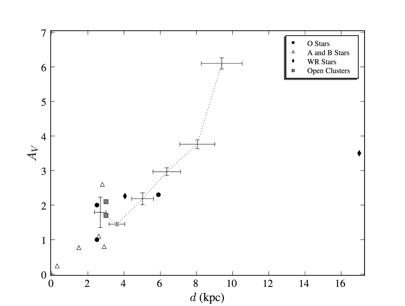
Figure 9: Comparison of reddening as a function of distance in the field of 1E 1048.1$-$5937 from the red-clump method (shown with error bars) with other reddening/distance determinations .

To check the performance of the red-clump method in this most complex of fields, we compare the function $A_{V}(d)$ found above with measured distances and reddenings of different types of source in the field: open clusters (from Loktin et al, 1994), Wolf-Rayet stars (van der Hucht, 2001), O-stars (from Garmany et al. 1982) and other early-type stars (Guarinos, 1992) within 40′of the source. Figure 9 shows all these data against the reddening curve found for 1E 1048.1$-$5937 above. Although, as shown in §3, there is a fair amount of scatter due to inhomogeneous reddening in the field, the general trend of reddening with distance is well-followed by all of the data-sets, with the notable exception of WR 29 (at large distance and low reddening). Crucially, none of them indicate the presence of $A_{V}>3$ up to 4 kpc, so the AXP would need a substantially lower column than that inferred from the X-ray spectrum in order to be at the distance of Gaensler et al’s interstellar bubble.

We also checked the extinction model of Drimmel et al. (2003) to see if their results were consistent with ours. We found that their predicted extinction along this line of sight is consistently higher than ours in the 4–8 kpc range. This is not surprising, given that we know from Gaensler et al. that the source lies through a hole in the interstellar extinction. The Drimmel et al. curve is consistent with curves 2, 3 and 4 from Figure 3.

5.3 1E 2259+586

The supernova remnant CTB 109, thought to be associated with the AXP 1E 2259+586, has been the subject of a number of studies to try to determine its distance and reddening, with range of previous distance estimates for the magnetar and SNR as about 3 to 7 kpc (Kothes et al. 2002, introduction). Most recently, Kothes et al. (2002) inferred that CTB 109 was at a distance of 3 kpc, from the following argument. The supernova remnant is apparently interacting with a large molecular cloud in the direction $l\approx 108.8\arcdeg$, $b\approx-0.9\arcdeg$. This cloud has a velocity of $-50{\rm\,km\,s^{-1}}$, which is similar to the range of $-30\ldots-55{\rm\,km\,s^{-1}}$ found for several H II regions within a few degrees of the remnant. For these latter regions, spectroscopic distance have been measured, which group around a distance $d=3\,$kpc. This is rather nearer by than expected based on the standard rotation curve for this direction, premably because of streaming motion known to be associated with the Perseus Arm shock.

A distance of 3 kpc for 1E 2259+586, however, is excluded by our analysis: at 3kpc, there are no red-clump stars sufficiently highly reddened to be consistent with 1E 2259+589’s column. One reason for the discrepancy might be that 1E 2259+589 is not associated with the SNR CTB 109. We believe this is unlikely, however, given both the positional coincidence and the morphology. Similarly, the shape of the remnant strongly suggests that it is indeed interacting with a dense molecular cloud positioned at the above mentioned co-ordinates.

Of the H II regions listed in Table 2 and shown in Figure 2 of Kothes et al. (2002), two have distances consistent with being behind the Perseus shock (Sh 149 and Sh 156, $d=4\ldots 8\,$kpc). Interestingly, among the 11 regions with velocities similar to the cloud with which CTB 109 appears to be interacting ($v<-40{\rm\,km\,s^{-1}}$), these two are amongst the three closest to CTB 109 on the sky.

Figures 4 and 5 of Kothes et al. (2002) show CO and H I data in the direction of CTB 109. From these figures, there appear to be two components to the CO cloud West of the SNR: one which includes the “arm” which passes across the SNR (with velocity $-47\ldots-51{\rm\,km\,s^{-1}}$) and a second which does not ($-53\ldots-56{\rm\,km\,s^{-1}}$) . These two components show different morphology and span a large range in velocity, suggesting that they are physically distinct. The H I data is less clear, but the morphology at $-55{\rm\,km\,s^{-1}}$ again seems match what one would expect from interaction with the supernova remnant. Since the remnant is known not to be interacting with the “arm” (see Sasaki et al. 2004), the above-described morphology suggests it is likely interacting with the second, more distant cloud.

A resolution to the distance discrepancy would thus be that the foreground cloud, including the “arm” which partially covers CTB 109, is indeed involved in streaming motion, but that CTB 109 is interacting with a background cloud unconnected with the first. If this background cloud is not associated with the streaming motion, but follows the standard rotation curve ($\Theta_{\odot}=220{\rm\,km\,s^{-1}}$, $R_{\odot}=8.5\,$kpc), then its distance is $\sim\!6\,$kpc, which is consistent with our estimate for the distance of 1E 2259+589.

Finally, as an independent check, we note that the Wolf-Rayet star WR 158, which is at an angular separation of 6.1°, has a spectroscopic distance of $\sim\!8\,$kpc and extinction $A_{V}\approx 4$ (van der Hucht, 2001). Another, WR 151, at a separation 6.8°, has $d\simeq 5.7\,$kpc and $A_{V}\approx 3.8$. These combinations of reddening and distance are consistent with our inferred run of reddening with distance (Fig. 7). Thus, we believe our distance estimate is reliable.

We check further that the red-clump method gives reasonable distances for objects of known reddening and distance in this part of the sky. The first object we check is Cas A, which is similar in some respects to CTB 109: it is a supernova remnant with a central compact X-ray source. The distance to Cas A is well known at $d=3.4^{+0.3}_{-0.1}$ kpc (Reed et al. 1995). Figure 10 shows the derived function $A_{V}(d)$ for 2000 stars within 10′of the position of Cas A. The reddening of the supernova remnant has been estimated from optical spectra and colors of various sections. The range of estimates of reddening is shown, which includes the majority of the estimates and the poorly measured hydrogen column for the central X-ray source (Fesen & Hurford, 1996; Fesen et al. 2006). (Some estimates lie outside this region, but we discount these extreme estimates). Clearly, the measured distance to the SNR is consistent with the reddening: our method gives a limit on the distance $d>1.9$ kpc. Were we trying to find the distance to Cas A, we would have reasoned that it must reside in the spiral arm (since it is also the product of a short-lived, massive star), close to its known distance (shown by the vertical dashed line).

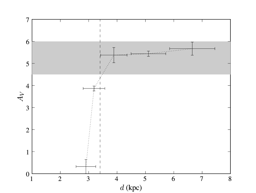
Figure 10: The red-clump method as applied to Cas A. The vertical dashed line is the estimated distance of Cas A, and the grey shaded region contains the majority of reddening estimates for the SNR and the central source (a range of estimates rather than the uncertainty on one estimate).

6 Implications

With our distances, X-ray luminosities for the AXPs can be calculated from their unabsorbed flux (taken when they were not thought to be in outburst; we use the numbers from Woods & Thomson, 2004). The results are listed in Table 2. For comparison, we also include two sources not considered above, CXOU J010043.1$-$721134 and SGR 0526$-$66, for which reasonably good distances are known since they are located in the SMC and LMC, respectively. Of these, the first is thought to be an AXP (Lamb et al. 2002; Majid et al. 2004) and the latter is a Soft Gamma-Ray Repeater (SGR), another class of magnetar.

From Table 2, one sees that all Galactic AXPs have remarkably similar X-ray luminosities. In part, this may be a coincidence: all sources are known to vary to some degree, and XTE J1810$-$197 is a transient. Furthermore, while for SGR 0526$-$66, which is clearly brighter, one might appeal to it being a different type of source (see also below), the one extra-galactic AXP, CXOU J010043.1$-$721134 in the SMC, is substantially fainter. Nevertheless, taken together, the luminosities listed in Table 2 suggests that the emission mechanism responsible for the persistent soft X-rays is self-limiting in the AXPs, despite differences in their spectra and timing properties.

This result was predicted. Thompson & Duncan (1996, §3.6) noted that the soft X-ray luminosity of a magnetar must saturate at a value near $L_{X}\simeq 10^{35}{\rm\,erg\,s^{-1}}$, because at higher luminosities neutrino emission from the interior would become dominant and cause rapid cooling. Here, the precise limiting luminosity could be greater by a factor of a few, depending on the surface composition (the above limit is for iron, C. Thompson 2006, pers. comm.). Furthermore, Arras et al. (2002) found, from considerations of the amibipolar diffusion time-scale of the magnetar’s internal magnetic field, that AXPs should remain near the limit for $10^{3}\dots 10^{5}\,$yr (i.e., the typical characteristic ages of the AXPs, Woods & Thompson 2004) before exhausting their internal heat supply and cooling rapidly by photon emission from the surface. Thus, it appears that the tight clustering in $L_{X}$ we find has a natural explanation in the context of the magnetar scenario. For a transient AXP, it would appear that the general luminosity is below the critical value, but that in outburst it is also limited by the threshold.

Table 2: Inferred quantities

Object	$L_{X}(2-10{\rm\,keV})$	$\frac{L_{\rm bb}^{\rm bol}}{L_{X}}$	$B_{\rm dipole}$	$T_{\rm bb}$	$R_{\rm bb}$	Pulsed Fraction
	($10^{35}{\rm\,erg\,s^{-1}}$)		($10^{14}$ G)	(keV)	(km)	(%RMS)
4U 0142+61	1.3	0.43	1.3	0.39	8.9	03.9
1E 1048.1$-$5937	1.4	0.13	3.9	0.63	1.7	62.4
1E 2259+589	1.3	0.11	0.6	0.41	4.2	23.2
1RXS J170849.0$-$400910	1.1	0.27	4.7	0.44	5.0	20.5
1E 1841$-$045	1.1	0.32	7.1	0.44	5.5	13.0
XTE J1810$-$197	1.3	0.56	02.9	0.67	2.6	42.8
CXOU J010043.1$-$721134	0.4	$\cdots$	4.5	0.41	$<\!7$	33.0
SGR 0526$-$66	2.6	0.06	7.4	0.53	2.6	04.8

Note. — The dipole magnetic field strength $B_{\rm dipole}$, black-body temperature $T_{\rm bb}$ and pulsed fraction are taken from the compilation of Woods & Thompson (2004). The black-body radius $R_{\rm bb}$ is calculated using the following fits: 0142, White et al. (1996); 1048, Mereghetti et al. (2004); 2259, Woods et al. (2004); 1708, Rea et al. (2003); 1841, Morii et al. (2003); 1810, Gotthelf et al. (2004); 0100, Lamb et al. (2002); 0526, Kulkarni et al. (2003). We do not list uncertainties, since these are dominated by source variability.

Typically, the soft X-ray spectra of the AXPs are fit with a composite model, consisting of a black-body and a power-law component. Presumably, the former arises from the neutron-star surface, and typically is responsible for the peak in the observed spectra. With our new distances, we can estimate the emitting area, or, equivalently, the effective black-body radius. This estimate should be fairly robust, since in essence it depends only on the wavelength and the measured flux of the spectral peak.

In Table 2, we list the inferred black-body radii for each of the AXPs, as well as a number of other physical parameters which one might expect to be related: the fraction of the total luminosity that is in the black-body component, the black-body temperature, the magnetic field strength inferred from the spin-down rate (assuming magnetic-dipole radiation), and the pulsed flux. All numbers were taken when the objects were thought to be in quiescence (with the exception of XTE J1810$-$197, which is a transient AXP).

From the Table, one sees that there is no obvious correlation with dipole magnetic field strenght, but the black-body radius and temperature are correlated, with temperature increasing for smaller effective radii. The strongest correlation, however, is between the pulsed fraction and black-body radius: they are well described by ${\rm PF}\propto R_{\rm bb}^{-2}$. This suggests an inverse proportionality of pulsed fraction with emitting area, as might be expected if different sources had, e.g., different sizes of the regions near the magnetic poles, where heat conduction is largest. (Such a correlation should break down for sources with hot poles close to the rotation axis, or the rotation axis close to the line of sight. But for random mutual inclinations, such geometries are relatively rare, so it is not surprising that our list does not include such an exception.) Our result also implies that any high-energy power-law component within the 2–10 keV band must be tied strongly to the thermal photon flux, since otherwise the correlation would be weakened.

An open question, though, is what causes the differences between the AXPs. In general, one might expect hotter, smaller surfaces for stronger magnetic fields, since stronger fields should lead to larger differences in heat conduction across and along magnetic field lines. But we do not find any correlation with the field strength inferred from the spin-down rate. One possibility is that the latter is not a good measure for the field strength at the surface, e.g., because the surface field is dominated by higher-order multipole components. For that case, however, one might expect to see more complicated pulse shapes than are typically observed. Another possibility would be that the magnetic field strengths are roughly dipolar, but offset from the center (as typically inferred for magnetic white dwarfs and Ap stars; e.g., Wickramasinghe & Ferrario 2000). If so, the AXPs with the largest pulsed fractions might have the largest offsets, for which the effects of partial overlap between polar caps might lead to smaller effective radii.

While the above correlations are intriguing, one sees from Table 2 that there is one exception, SGR 0526$-$66. This object, although discovered in 1979 as the first SGR through its gamma-ray outbursts, is the most AXP-like of its class in its timing and spectral properties (Kulkarni et al. 2003). Yet, it flouts both the temperature and black-body radius correlations with pulsed fraction, and has a higher 2–10 keV luminosity than the limit inferred for the AXPs. The luminosity of the black-body component alone, however, is in the same range as for the AXPs. If the emission source for the thermal component is the same as it is for the AXPs, this suggests that the non-thermal component is powered at least partly from another, additional reservoir of energy. For instance, the energy could be stored in a large magnetic twist imparted during the previous gamma-ray bursting phase. Such magnetic twists are thought to decay on time scales of the order decades (Beloborodov & Thompson 2006), so it is possible that SGR 0526$-$66 has not yet returned to a quiescent, AXP-like state.

Intriguingly, it would seem that the AXPs, particularly 1E 1048.1$-$5937 and 1E 2259+586 seem to be located through gaps in the interstellar extinction. This likely is selection effect: the objects are detected primeraly in the soft X-ray band due to the sensitivities of the main X-ray observatories, and the X-ray spectra of the AXPs fall rapidly in the 2–10 keV range. The only two AXPs with estimated hydrogen columns $N_{H}>1.5\times 10^{22}$ cm^-2, 1E 1841$-$045 and AX J1845$-$0258 were discovered through observations of the SNRs Kes 73 and Kes 75 respectively (Kriss et al. 1985; Gotthelf & Vasisht, 1998). This suggests that there may be many more AXPs in the Galaxy, which have not been discovered so far due to high extinction. They could, however, be discovered by their high-energy ($>$20 keV) emission, if it exists and is pulsed, as has been found for the AXPs detected by INTEGRAL so far (Kuiper et al. 2006).

7 Conclusions

We have applied the “red-clump” method to 2MASS data to construct the run of reddening versus distance in the directions of each of the Galactic AXPs. Combined with estimates of the reddenings to the AXPs, half of which are from our recent, model-independent determinations from photo-electric absorption edges in high-resolution X-ray spectra, we inferred distances. We found that two of these estimated distances are inconsistent with ones in the literature, but found likely reasons for the discrepancy in both cases and concluded that our results were reliable.

From the reddening versus distance diagrammes, we find that the AXPs tend to fall in regions of rapidly rising reddening that are associated with spiral arms. This is not surprising, since they are the young remnants of short-lived massive stars. In particular, 4U 0142+61 has a position consistent with the Perseus Arm, 1E 1048.1$-$5937 lies on the far side of the Carina Arm, and 1XTE J1810$-$197 and 1RXS J170849.0$-$400910 fall along the Crux-Scutum arm. 1E 1841$-$045 could either lie in the Scutum arm or in the Molecular Ring, which dominates the gas and dust density at galactocentric distances of about 4 kpc (Dame et al. 2001). 1E 2258+586 falls near the end of the Outer Arm, known to exist in this direction beyond the Perseus arm (e.g., Kimeswenger & Weinberger 1989).

From our distances, we infer 2–10 keV luminosities and we find that these cluster tightly around $1.3\times 10^{35}{\rm\,erg\,s^{-1}}$, consistent with the prediction in the context of the magnetar model that a saturating luminosity must exist above which rapid internal neutrino cooling is effective. Furthermore, we calculated effective emitting radii for the thermal components in the X-ray spectra, and find that these are inversely correlated with temperature, while the corresponding areas are inversely proportional to the pulsed fraction. This suggests the internal heating is released predominantly through one or more hot polar caps, with sizes that differ between the different AXPs.

The red-clump method can be applied to any line of sight in the Galactic plane, and is particularly useful combined with reddening estimates from X-ray spectroscopy. More accurate results may be obtained using deeper infrared imaging of selected fields, although, unfortunately, it may not be possible to extend the method to regions with very high reddening, since the red clump stars may well become confused with highly reddened main-sequence stars. As a result of the latter limitation, the method may not be generally useful for the other class of magnetars, the soft gamma-ray repeaters, which generally suffer very high extinction. It should be useful, however, for point sources such as the Compact Central Objects.

Generally, for further analysis of distances and structure within the Milky Way, it would be useful to cross-calibrate results from the red-clump method with those from X-ray absorption studies, X-ray dust scattering haloes, and H I and CO measurements.

Acknowledgments: We would like to acknowledge the thoroughness and many useful suggestions and comments of the anonymous referee. We thank David Kaplan for pointing out the paper describing the red-clump method to us, and Martin López-Corredoira for information on the applicability of the red-clump method. We also thank Bryan Gaensler for help with interpreting CO and H I data and for discussions about 1E 1048.1$-$5937, Manami Sasaki and Terrance Gaetz for discussing the case of CTB 109, and Tom Dame and Peter Martin for general discussions of Galactic gas and dust. This publication makes use of the Two Micron All Sky Survey, which is a joint project of the University of Massachusetts and the Infrared Processing and Analysis Center/California Institute of Technology, funded by NASA and NSF. We acknowledge financial support from NSERC.

References

- (1) Arras, P., Cumming, A., Thompson, C., 2004, ApJ, 608, L49
- (2) Beloborodov, A. & Thompson, T., 2006, arxiv:astro-ph/0602417
- (3) Cordes, J., & Lazio, T., 2002, arxiv:astro-ph/0207156
- (4) Dame, T., Hartmann, D. & Thaddeus, P., 2001, ApJ, 547, 792
- (5) Drimmel, R., Cabrera-Lavers, A., López-Corredoira, M, 2003, A&A, 409, 205
- (6) Durant, M., & van Kerkwijk, M., 2005, ApJ, 627, 376
- (7) Durant, M., & van Kerkwijk, M., 2006, ApJ, submitted
- (8) Fesen, R., Hurford, A., 1996, ApJS, 106, 563
- (9) Fesen, R., Pavlov, G., Sanwal, D., 2006, ApJ, 636, 848
- (10) Gaensler, B., McClure-Griffiths, N., Oey, M., Haverkorn, M., Dickey, J., Green, A., 2005, ApJ, 620, L95
- (11) Garmany, C., Conti, P., Chiosi, C., 1982, ApJ, 263, 777, Vizier on-line catalogue II/82
- (12) Gotthelf, E., Halpern, J., Buxton, M., Bailyn, C., 2004, ApJ, 605, 368
- (13) Gregory, P., Fahlman, G., 1980, Nature, 287, 805
- (14) Guarinos, 1992, Ph.D. Thesis, Strasbourg Observatory, Vizier on-line catalogue V/86
- (15) Hulleman, F., van Kerkwijk, M., & Kulkarni, S., 2004, A&A, 416, 1037
- (16) Kimeswenger, S., Weinberger, R., 1989, A&A, 209, 51
- (17) Kothes, R., Uyaniker, B., Yar, A., 2002, ApJ, 576, 169
- (18) Kriss, G., Becker, R., Helfand, D., Canizares, C., 1985, ApJ, 28, 703
- (19) Kulkarni, S., Kaplan, D., Marshall, H., Frail, D., Murakami, T., Yonetoku, D., 2003, ApJ, 585, 948
- (20) Lamb, R., Fox, D., Macomb, D., Prince, T., 2002, ApJ, 574, L29
- (21) López-Corredoira, M., Labrera-Lavers, A., Garzón, F., & Hammersley, P., 2002, A&A, 394, 883
- (22) Loktin, A., Matkin, N., Gerasimenko, T., 1994, A&A T 4, 153, Vizier on-line catalogue V/96
- (23) Majid, W,. Lamb, R., & Malcolm, D, 2004, ApJ, 609, 133
- (24) Mathis, J., 1990, ARA&A, 28, 37
- (25) Mereghetti, S., Tiengo, A., Stella, L., Israel, G., Rea, N., Zane, S., Oosterbroek, T., 2004, ApJ, 608, 427
- (26) Morii, M., Sato, R., Kataoka, J., Kawai, N., 2003, PASJ, 55, L45
- (27) Muno, M., Clark, S., Crowther, P., Dougherty, S., de Grijs, R., Law, C., McMillan, S., Morris, M., Negueruela, I., Pooley, D., Portegies Zwart, S., Yusef-Zadeh, F., 2006, ApJ, 636, L41
- (28) Persson, S., Murphy, D., Gunnels, S., Birk, C., Bagish, A., Kock, E., 2002, ApJ, 124, 619
- (29) Predehl, P., & Schmitt, J., 1995, A&A, 293, 889
- (30) Rea, N., Israel, G., Stella, L., Oosterbroek, T., Mereghetti, S., Angelini, L., Campana, S., Covino, S., 2003, ApJ, 586, L65
- (31) Reed, J., Hester, J., Fabian, A., Winkler, P., 1995ApJ…440..706
- (32) Sanbonmatsu, K., Helfand, D., 1992, AJ, 104, 2189
- (33) Sasaki, M., Plucinsky, P., Gaetz, T., Smith, R., Edgar, R., Slane, P., 2004, ApJ, 617, 322
- (34) Schlegel, D., Finkbeiner, D., & Davis, M. 1998, ApJ, 500, 525
- (35) Skrutskie, M., Cutri, R., Stiening, R., Weinberg, M., Schneider, S., Carpenter, J., Beichman, C., Capps, R., Chester, T., Elias, J., Huchra, J., Liebert, J., Lonsdale, C., Monet, D., Price, S., Seitzer, P., Jarrett, T., Kirkpatrick, J., Gizis, J., Howard, E., Evans, T., Fowler, J., Fullmer, L., Hurt, R., Light, R., Kopan, E., Marsh, K., McCallon, H., Tam, R., Van Dyk, S., Wheelock, S., 2006, AJ, 131, 1163
- (36) Thompson, C. & Duncan, R., 1996, ApJ, 473, 322
- (37) van der Hucht, K., 2001, New Astronomy Reviews, 45, 135 (Issue 3)
- (38) Vasisht, G., Gotthelf, E., 1997, ApJ, 486, L129
- (39) Vink, J., Kuiper, L., 2006, MNRAS accepted, astro-ph/0604187
- (40) Wainscoat, R., Cowie, L., 1992, AJ, 103, 332
- (41) White, N., Angelini, L., Ebisawa, K., Tanaka, Y., Ghosh, P., 1996, ApJ, 463, L83
- (42) Wickramasinghe, D. T., & Ferrario, L., 2000, PASP, 112, 873
- (43) Woods, P., Kaspi, V., Thompson, C., Gavriil, F., Marshall, H., Chakrabarty, D., Flanagan, K., Heyl, J., Hernquist, L., 2004, ApJ, 605, 378
- (44) Woods, P., & Thompson, C., 2004, in “Compact stellar X-ray sources”, eds Lewin, W., van der Klis, M.