High-energy Emission from Pulsar Magnetospheres

Abstract

A synthesis of the present knowledge on gamma-ray emission from the magnetosphere of a rapidly rotating neutron star is presented, focusing on the electrodynamics of particle accelerators. The combined curvature, synchrotron, and inverse-Compton emission from ultra-relativistic positrons and electrons, which are created by two-photon and/or one-photon pair creation processes, or emitted from the neutron-star surface, provide us with essential information on the properties of the accelerator — electric potential drop along the magnetic field lines. A new accelerator model, which is a mixture of traditional inner-gap and outer gap models, is also proposed, by solving the Poisson equation for the electrostatic potential together with the Boltzmann equations for particles and gamma-rays in the two-dimensional configuration and two-dimensional momentum spaces.

Modern Physics Letters A

Received: 01 May 2006

Accepted: 09 May 2006

1 Pulsar nature and characteristics

When a star has exhausted its nuclear fuel, the interior thermal pressure can no longer support its own weight. If the star is not very massive, it collapses to the point at which electron degeneracy pressure halts gravitational collapse, and a white dwarf is formed. However, beyond the critical mass [1], even the electron degeneracy pressure becomes insufficient to support the star. In the collapsing stellar core, most of the electrons are absorbed by protons via inverse $\beta$ decay and eventually the neutron degeneracy pressure halts the gravitational collapse [2, 3, 4]. For a progenitor star to collapse directly to a neutron star, its mass should be more than $10$ times greater than our Sun. A neutron star, which can rotate with a period as fast as $P\sim 1$ ms, is considered to be the only candidate for the source of remarkably stable radio pulses, of which fastest period is 1.55 ms (PSR J1939+2134 [5]). When it was determined that the period of the Crab pulsar was slowly increasing [6], the identification of pulsars as rapidly rotating neutron stars was essentially confirmed [7, 8].

Having established pulsars as rotating neutron stars, the next thing to discuss is the pulsar characteristics deduced from observations. Since all known isolated pulsars show gradual spin down, there must be some mechanisms causing the neutron star to lose their rotational energy. The rotational energy-loss rate is given by

$$\dot{E}=I\Omega\dot{\Omega}=-(2\pi)^{2}I\dot{P}/P^{3},$$ (1)

where the neutron star is rotating with angular frequency $\Omega=2\pi/P$ and moment of inertia $I$. For typical high-energy pulsars, $P\sim 0.1$ s, $\dot{P}\sim 10^{-13}\,\mbox{s s}^{-1}$, $I\sim 10^{45}\mbox{g\,cm}^{2}$; thus, we obtain $\dot{E}=-4\times 10^{36}\,\mbox{ergs s}^{-1}$, which is enough to explain the observed $\gamma$-ray luminosities, $10^{32.5}\,\mbox{ergs s}^{-1}<L_{\gamma}<10^{35}\,\mbox{ergs s}^{-1}$. For an object as small as $r_{\ast}\sim 10$ km in radius to experience such a large torque, it must have a strong coupling to their surroundings, most likely through magnetic fields intrinsic to the neutron star. If the neutron star is losing its rotational energy via magnetic dipole radiation, the spin-down luminosity is given by

$$L_{\rm dip}=k\Omega^{4}\mu^{2}/c^{3},$$ (2)

where $k=2\sin^{2}\alpha_{\rm i}/3$ is commonly used for a vacuum rotating magnetic dipole with inclination $\alpha_{\rm i}$ with respect to the rotation axis. Equating $L_{\rm dip}$ with $-\dot{E}$, we can infer the magnetic moment, $\mu$, of the star [9]. For $P=0.1$ s, $\dot{P}=10^{-13}\,\mbox{s s}^{-1}$, $I=10^{45}\mbox{g\,cm}^{2}$, we obtain $\mu=2.6\times 10^{30}\,\mbox{G cm}^{3}$ and the surface magnetic field strength, $B_{\ast}=5.2\times 10^{12}(r_{\ast}/10\mbox{km})^{-3}$ G, as the Newtonian value at the magnetic pole. In what follows, we consider possible emission models of isolated, rotating neutron stars, after briefly mentioning the high-energy observations.

2 Gamma-ray observations and physical processes

The Energetic Gamma Ray Experiment Telescope and the imaging Compton Telescope aboard the Compton Gamma Ray Observatory have detected pulsed signals from at least seven rotation-powered pulsars (Crab pulsar [10, 11]; PSR B1509-58 [12]; Vela pulsar [13, 11]; PSR B1706-44 [14]; PSR B1951+32 [15]; Geminga pulsar [16, 11]; PSR B1055-52 [17]). Four of them (Crab, Vela, Geminga, and B1951+32) exhibit double-peaked light curves[18, 19, 20] (fig. 1). Since interpreting $\gamma$-rays should be less ambiguous compared with reprocessed, non-thermal X-rays, the $\gamma$-ray pulsations observed from these objects are particularly important as a direct signature of basic non-thermal processes in pulsar magnetospheres.

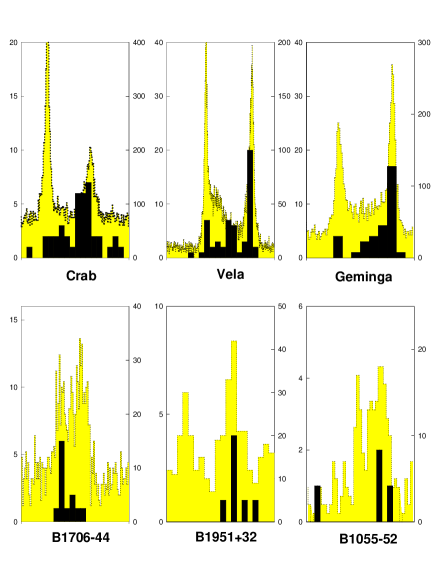
Figure 1: Light curves of six $\gamma$-ray pulsars above 100 MeV (dotted lines, right-hand scale) and above 5 GeV (dark histogram, left-hand scale). Each panel shows one full rotation of the neutron star. From Thompson (2004).

Spectral energy distributions (SEDs) offers the key to an understanding of the radiation processes. Ref. [17] compiled a useful set of broad-band SED for the seven $\gamma$-ray pulsars. The most striking feature of these $\nu F_{\nu}$ plots is the flux peak above 0.1 GeV with a turnover at several GeV. Various models [21, 22, 23, 24, 25, 26] conclude that these photons are emitted by the electrons or positrons accelerated above 5 TeV via curvature process. Such ultra-relativistic particles could also cause inverse-Compton (IC) scatterings. In particular, for young pulsars, their strong thermal X-rays emitted from the cooling neutron-star surface [27, 28, 29] efficiently illuminate the gap to be upscattered into several TeV energies. If their magnetospheric infrared (0.1–0.01 eV) photon field is not too strong, a pulsed IC component could be unabsorbed to be detected with future ground-based or space telescopes.

The curvature-emitted photons have the typical energy of a few GeV. Close to the star (typically within a few stellar radii), such $\gamma$-rays can be absorbed by the strong magnetic field ($>10^{12}$ G) to materialize as a pair. On the other hand, outside of this strong-field region, pairs are produced only by the photon-photon collisions (e.g., between the curvature-GeV photons and surface- or magnetospheric- keV photons). The replenished charges partially screen the original acceleration field, $E_{\parallel}$. If the created particles pile up at the boundaries of the potential gap, they will quench the gap eventually. Nevertheless, if the created particles continue to migrate outside of the gap as a part of the global flows of charged particles, a steady charge-deficient region will be maintained. This is the basic idea of a particle acceleration zone in a pulsar magnetosphere.

3 Representative emission models

The pulsar magnetosphere can be divided into two zones: The closed zone filled with a dense plasma corotating with the star, and the open zone in which plasma flows along the open field lines to escape through the light cylinder (left panel of fig. 2). These two zones are separated by the the last-open magnetic field lines, which become parallel to the rotation axis at the light cylinder. Here, the light cylinder is defined as the surface where the corotational speed of a plasma would coincide with the speed of light, $c$, and hence its distance from the rotation axis is given by $\varpi_{\rm LC}\equiv c/\Omega$. If a plasma flows along the magnetic field line, causality requires that the plasma should migrate outward outside of the light cylinder. In all the pulsar emission models, particle acceleration takes place within the open zone.

For an aligned rotator (i.e., $\sin\alpha_{\rm i}=0$), open zone occupies the magnetic colatitudes (measured from the magnetic axis) that is less than $\sqrt{r_{\ast}/\varpi_{\rm LC}}$. For an oblique rotator, even though the open-zone polar cap shape is distorted, $\pi(r_{\ast}/\varpi_{\rm LC})$ gives a good estimate of the polar cap area. On the spinning neutron star surface, from the magnetic pole to the rim of the polar cap, an electro-motive force, $\approx\Omega^{2}B_{\ast}r_{\ast}^{3}/c^{2}\approx 10^{16.5}$ V, is exerted. This strong EMF causes the magnetospheric currents that flow outwards in the lower latitudes and inwards along the magnetic axis (center panel in fig. 2). The return current is formed at large-distances where Poynting flux is converted into kinetic energy of particles or dissipated [30].

           

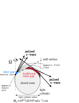
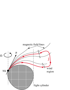
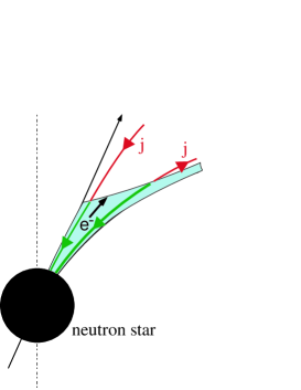
Figure 2: Sideview of pulsar magnetosphere. Left: two representative accelerator models in the open zone; center: global electric current due to the EMF exerted on the spinning neutron star surface when $\mbox{\boldmath$\Omega$}\cdot\mbox{\boldmath$\mu$}>0$; right: current derived in the inner-slot-gap model (green arrow, see § 6.4).

Attempts to model the particle accelerator have traditionally concentrated on two scenarios: Inner-gap models with emission altitudes of $\sim 10^{4}$cm to several neutron star radii over a pulsar polar cap surface [31, 32, 21, 33, 34] and outer-gap models with acceleration near the light cylinder [35, 36, 37, 38, 39]. It is worth noting that average location of energy loss should take place near the light cylinder so that the rotating neutron star may lose enough angular momentum [40], which indicates the existence of the inner gap must affect the electrodynamics in the outer magnetosphere.

It is widely accepted from phenomenological studies that coherent radio pulsations are probably emitted from the inner gap that is located near the magnetic pole. Moreover, coherent radio pulsations provide the primary channel for pulsar discovery (1560 pulsars as of April 2006, see ATNF pulsar catalogue, http://www.atnf.csiro.au/research/pulsar/psrcat/). However, it is, unfortunately, very difficult to reproduce them by considering plasma collective effects. Therefore, in this review, I will focus on incoherent high-energy, non-thermal radiation, which is the product of magnetospheric gaps.

It is worth mentioning other models than the inner and outer gap models. A charge depletion can alternatively be a consequence of a stable charge void (i.e., no plasma region with $\mbox{\boldmath$B$}\cdot\mbox{\boldmath$E$}\neq 0$) in a neutron-star magnetosphere [41, 42, 43]. Even though their works provides important hints on electrostatics, I do not intend to speculate on the dynamics of the formation of the void, to take account of magnetospheric currents, which are not considered in their works. There is another model that radiation takes place in a pulsar wind at roughly 10 to 100 light cylinder radii from the star as a result of the magnetic energy dissipation [44, 45, 46], which is a reexamination of the non-axisymmetric striped pulsar wind [47, 48]. However, to discuss the reconnection in a relativistic plasma is beyond the scope of this brief review.

4 Magnetospheric current determination

We briefly discuss how to determine the magnetospheric current. Adopting the force-free limit (i.e., neglecting plasma inertia), Ref. [49] solved the Grad-Shafranov (GS) Eq. [50, 51, 52] $(x^{2}-1)(\partial_{x}^{2}+\partial_{z}^{2})P+(x+1/x)\partial_{x}P=j\,dj/dP$, to obtain the magnetic flux function $P$, which determines the fieldline configuration, where $x$ and $z$ denote the distances from the rotation axis and the equatorial plane, respectively, in $\varpi_{\rm LC}$ unit, and $j$ the magnetospheric current on the poloidal (i.e., meridional) plane. This work inaugurated numerous attempts [53, 54, 55, 56] on solving the GS Eq. in recent several years, and $k\approx 1+\sin^{2}\alpha_{\rm i}$ is suggested in Eq. (2), by determining $j(P)$. However, it is noteworthy that they determined $j$ by imposing a continuity of $P$ at the turning point $x=1$ (i.e., the light cylinder), and by simply neglecting the highest-oder term at $x=1$ (including a regular Taylor expansion, which gives only one of the two independent solution bases if we suppress the $z$ dependence). Instead, we can adopt a singular perturbation theory to stretch the region $x\approx 1$ by transforming $P=Q/(x-1)$. Then there appears no singularity in the highest-order derivative term [57]. To find a particular solution, we can, for example, introduce a regulator such that $P=Q/[x-1-\epsilon(z)]$, recovering the imaginary part by Fourier analysis from the equations of force-free electrodynamics [58, 55], where $Q$ satisfies the GS Eq. without $z$ derivatives and $\epsilon$ is a small complex function. In this case, $x=1+\mbox{Re}(\epsilon)$ will give the Alfvénic separatrix surface [59, 60, 61], after recovering particle inertia. Any way, we must connect the interior solution with the asymptotic ones in $x<1$ and $x>1$. It means that $j$, a free parameter in the force-free framework, cannot be constrained by the continuity of $P$ at $x=1$, but should be determined by the global requirement including the dissipative region, which gives the electric load in the current circuit within the sub-fast-magnetosonic region (extended to large distances in a magnetically dominated magnetosphere) from causality requirement.

5 Geometrical consideration

In this section, we compare the emission geometry of a few representative gap models. For this purpose, we assume that the photons are outwardly emitted along the local magnetic field direction in the corotating frame of the magnetosphere. Then the lightcurve morphologies are subject to the general relativistic corrections (i.e., field distortion and light path bending near the star) and the special relativistic corrections (i.e., aberration of light, time-of-flight delays, and field retardation near the light cylinder). Aberration and time-of-flight delays leads to comparable phase shifts, $\sim-\varpi/\varpi_{\rm LC}$ at distance $\varpi$ from the rotation axis. On the leading side (left panel of fig. 3), these phase shifts add up to spread photons emitted at various altitudes over $0.4$ in phase. On the other hand, on the trailing side (right panel), photons emitted later at higher altitudes catch up with those emitted earlier at lower altitudes, arriving at an observer within a small phase range $0.1$ and produce caustics [62, 39] in the phase plot and light curves [63, 64].

A single inner-gap beam, which is emitted from the lower altitudes, can produce a variety of pulse profiles. The top left panel in Fig. 4 represents the phase plot, — photon intensity in the direction specified by $\Phi$ (pulse-phase) and $\zeta$ (observer’s viewing angle with respect to the rotation axis). An observer at $\zeta$ detects photon flux indicated by the shade at each pulse phase (bottom left panel). Because $E_{\parallel}$ fades away near the perfectly conducting edge of the open zone, the gap is shorter near the pole and extends to higher altitude near the rim (right panel). Faint off-beam curvature radiation above the gap can be seen outside the main beam, as the faintly shaded regions indicate[65]. A great deal of effort has been made on the inner-gap model [66, 67, 68, 69, 70]; however, one has to invoke a very small inclination angle to reproduce the wide separation of the two peaks (fig. 1). Thus, a high-altitude emission drew attention as an alternative possibility.

Assuming that the gap extends from the stellar surface to the light cylinder and that the photon emissivity is uniform within the gap, Ref. [64] demonstrated the formation of the double peaks arising from a crossing two caustics, each of which is associated with a different magnetic pole (fig. 5). Subsequently, Ref. [71] examined polarization characteristics and found that fast swings of the position angle and minima of polarization degree can be qualitatively reproduced within their two-pole caustic model. This type of emission — slot gap emission [72] — fills the whole sky and all phases in a lightcurve. Most observers will catch emission from the two poles if $\alpha_{\rm i}\geq 30^{\circ}$ (for $45^{\circ}\leq\zeta\leq 125^{\circ}$ in fig. 5). The dark features show the accumulation of photons because of the trailing side caustics (e.g., the thick curve at $\zeta<130^{\circ}$ and $|\Phi|<50^{\circ}$), and because of the overlap between the trailing side of pole 1 and the leading side of pole 2 near the light cylinder (e.g., the thinner branch of the Y feature at $50^{\circ}<\zeta<90^{\circ}$ and $50^{\circ}<\Phi<110^{\circ}$). The main peaks come from the trailing side of each pole, interpeak emission from the leading sides.

Geometrically speaking, an outer gap can be classified as a subset of the slot gap extended above the null surface. An observer can see, in this case, emission from the two outer gaps associated with only one pole. For example, in Fig. 6, if $\zeta=80^{\circ}$, the dotted line shows that we observe the photons emitted from the two outer gaps (shaded regions in the right panel) associated with the pole 2. There is no emission outside the sharp peak edges; thus, the emission is invisible at $\zeta<30^{\circ}$ or $\zeta>150^{\circ}$ for any obliquity. The first peak originate near $0.9\varpi_{\rm LC}$ (upper shaded region in the right panel), while the second peak caustic is formed by the photons emitted from the trailing field lines (lower shaded region in the right panel).

         

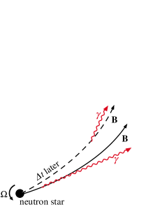
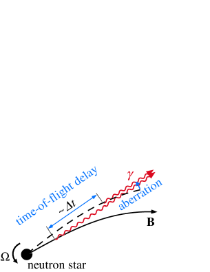
Figure 3: Photon propagation direction in a rotating neutron-star magnetosphere (top view). Left: Leading side emission, which forms weak photon intensity; right: Trailing side emission, which forms a caustic — piling up of photons emitted at different altitudes.

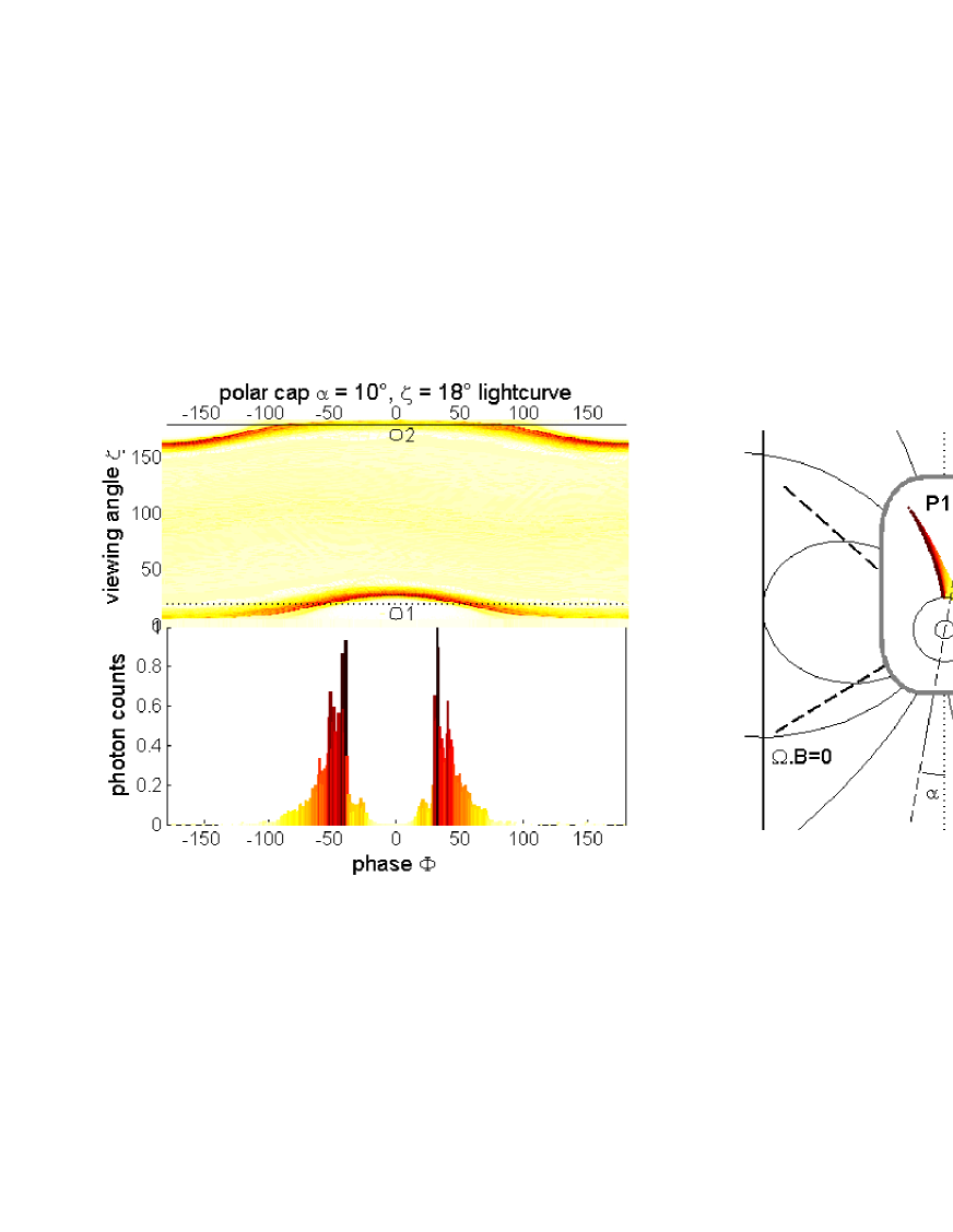
Figure 4: Phase plot, sample lightcurve, and a sketch of the accelerator location for the inner-gap model, for a typical inclination angle $\alpha_{\rm i}=10^{\circ}$. the central zoom gives the gap extent relative to the star size. the dashed lines outline the null surface. the shading in the lightcurve and gap sketch is the same. the phase plot illustrates the change in lightcurve as seen by different observers and the aperture of the pulsed beams. From Grenier and Harding (2006).

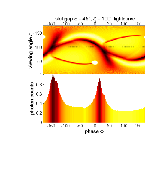
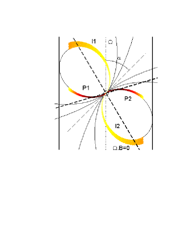
Figure 5: Same figure as fig. 1 for the slot-gap model, for a typical inclination angle $\alpha_{\rm i}=45^{\circ}$. From Grenier and Harding (2006).

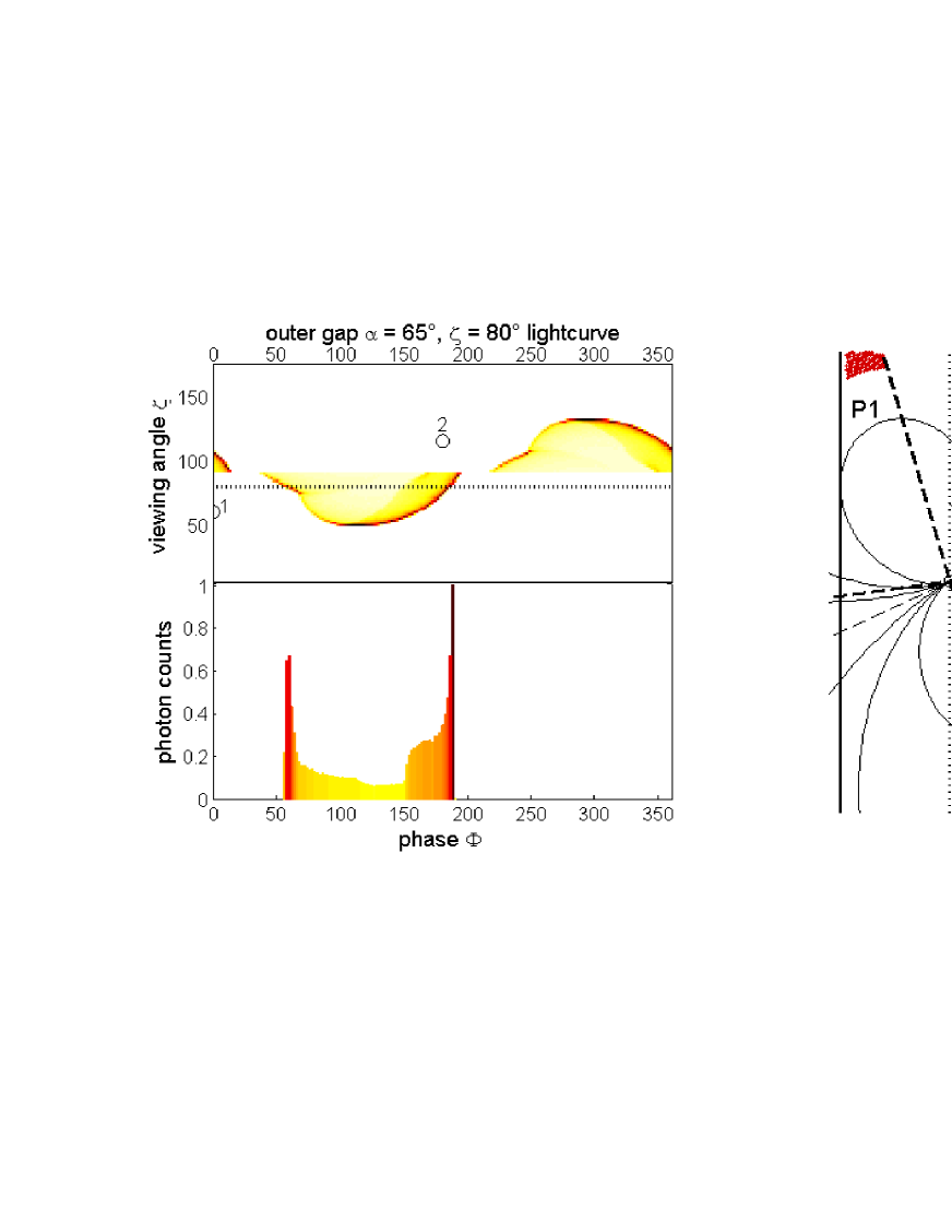
Figure 6: Same figure as fig. 1 for the outer-gap model, for a typical inclination angle $\alpha_{\rm i}=65^{\circ}$. From Grenier and Harding (2006).

6 Electrodynamical consideration

Next, let us consider the physical basis of the geometrical models discussed in § 5. To this aim, we have to derive the Poisson Eq. for the non-corotational potential, which is applicable to arbitrary gap models.

6.1 Poisson Equation for Electrostatic Potential

Around a rotating neutron star with mass $M$, the background space-time geometry is given by [73]

$$ds^{2}=g_{tt}dt^{2}+2g_{t\varphi}dtd\varphi+g_{rr}dr^{2}+g_{\theta\theta}d\theta^{2}+g_{\varphi\varphi}d\varphi^{2},$$ (3)

where

$$g_{tt}\equiv\left(1-\frac{r_{\rm g}}{r}\right)c^{2},\,g_{t\varphi}\equiv ac\frac{r_{\rm g}}{r}\sin^{2}\theta,$$ (4)

$$g_{rr}\equiv-\left(1-\frac{r_{\rm g}}{r}\right)^{-1},\,g_{\theta\theta}\equiv-r^{2},\,g_{\varphi\varphi}\equiv-r^{2}\sin^{2}\theta;$$ (5)

$r_{\rm g}\equiv 2GM/c^{2}$ indicates the Schwarzschild radius, and $a\equiv I\Omega/(Mc)$ parameterizes the stellar angular momentum. At radial coordinate $r$, the inertial frame is dragged at angular frequency $\omega\equiv-g_{t\varphi}/g_{\varphi\varphi}=0.15\Omega I_{45}r_{6}{}^{-3}$, where $I_{45}\equiv I/10^{45}\mbox{ erg cm}^{2}$, and $r_{6}\equiv r_{\ast}/10\,\mbox{km}$.

Let us consider the Gauss’s law,

$$\nabla_{\mu}F^{t\mu}=\frac{1}{\sqrt{-g}}\partial_{\mu}\left[\frac{\sqrt{-g}}{\rho_{\rm w}^{2}}g^{\mu\nu}(-g_{\varphi\varphi}F_{t\nu}+g_{t\varphi}F_{\varphi\nu})\right]=\frac{4\pi}{c^{2}}\rho,$$ (6)

where $\nabla$ denotes the covariant derivative, the Greek indices run over $t$, $r$, $\theta$, $\varphi$; $\sqrt{-g}=\sqrt{g_{rr}g_{\theta\theta}\rho_{\rm w}^{2}}=cr^{2}\sin\theta$ and $\rho_{\rm w}^{2}\equiv g_{t\varphi}^{2}-g_{tt}g_{\varphi\varphi}$, $\rho$ the real charge density. The electromagnetic fields observed by a distant static observer are given by [74, 75] $E_{r}=F_{rt},\,E_{\theta}=F_{\theta t},\,E_{\varphi}=F_{\varphi t}$, $B^{r}=(g_{tt}+g_{t\varphi}\Omega)F_{\theta\varphi}/\sqrt{-g},\,B^{\theta}=(g_{tt}+g_{t\varphi}\Omega)F_{\varphi r}/\sqrt{-g},\,B_{\varphi}=-\rho_{\rm w}^{2}F_{r\theta}/\sqrt{-g}$, where $F_{\mu\nu}\equiv\partial_{\mu}A_{\nu}-\partial_{\nu}A_{\mu}$ and $A_{\mu}$ denotes the vector potential.

Assuming that the electromagnetic fields are unchanged in the corotating frame, we can introduce the non-corotational potential $\Psi$ such that

$$F_{\mu t}+\Omega F_{\mu\varphi}=-\partial_{\mu}\Psi(r,\theta,\varphi-\Omega t),$$ (7)

where $\mu=t,r,\theta,\varphi$. If $F_{At}+\Omega F_{A\varphi}=0$ ($A=r,\theta$) holds, $\Omega$ is conserved along the field line. On the neutron-star surface, we impose $F_{\theta t}+\Omega F_{\theta\varphi}=0$ (perfect conductor) to find that the surface is equi-potential, that is, $\partial_{\theta}\Psi=\partial_{t}\Psi+\Omega\partial_{\varphi}\Psi=0$ holds. However, in a particle acceleration region, $F_{At}+\Omega F_{A\varphi}$ deviates from $0$ and the magnetic field does not rigidly rotate. The deviation is expressed in terms of $\Psi$, which gives the strength of the acceleration electric field that is measured by a distant static observer as

$$E_{\parallel}\equiv\frac{\mbox{\boldmath$B$}}{B}\cdot\mbox{\boldmath$E$}=\frac{B^{i}}{B}(F_{it}+\Omega F_{i\varphi})=\frac{\mbox{\boldmath$B$}}{B}\cdot(-\nabla\Psi),$$ (8)

where the Latin index $i$ runs over spatial coordinates $r$, $\theta$, $\varphi$.

Substituting Eq. (7) into (6), we obtain the Poisson equation for the non-corotational potential,

$$-\frac{c^{2}}{\sqrt{-g}}\partial_{\mu}\left(\frac{\sqrt{-g}}{\rho_{\rm w}^{2}}g^{\mu\nu}g_{\varphi\varphi}\partial_{\nu}\Psi\right)=4\pi(\rho-\rho_{{\rm GJ}}),$$ (9)

where the general relativistic Goldreich-Julian charge density is defined as

$$\rho_{{\rm GJ}}\equiv\frac{c^{2}}{4\pi\sqrt{-g}}\partial_{\mu}\left[\frac{\sqrt{-g}}{\rho_{\rm w}^{2}}g^{\mu\nu}g_{\varphi\varphi}(\Omega-\omega)F_{\varphi\nu}\right].$$ (10)

If $\rho$ deviates from $\rho_{{\rm GJ}}$ in any region, $E_{\parallel}$ is exerted along $B$. In the limit $r\gg r_{\rm g}$, Eq. (10) reduces to the ordinary, special-relativistic expression [76, 77],

$$\rho_{{\rm GJ}}\equiv-\frac{\mbox{\boldmath$\Omega$}\cdot\mbox{\boldmath$B$}}{2\pi c}+\frac{(\mbox{\boldmath$\Omega$}\times\mbox{\boldmath$r$})\cdot(\nabla\times\mbox{\boldmath$B$})}{4\pi c}.$$ (11)

Instead of ($r$,$\theta$,$\varphi$), it is convenient to adopt the so-called ‘magnetic coordinates’ ($s$,$\theta_{\ast}$,$\varphi_{\ast}$) such that $s$ denotes the distance along the magnetic field line, $\theta_{\ast}$ and $\varphi_{\ast}$ the magnetic colatitude and the magnetic azimuth of the point where the field line intersects the stellar surface. Defining that $\theta_{\ast}=0$ corresponds to the magnetic axis and that $\varphi_{\ast}=0$ to the plane on which both the rotation and the magnetic axes reside, we obtain the following form of Poisson Eq., which can be applied to arbitrary magnetic field configurations [78]:

$$-\frac{c^{2}g_{\varphi\varphi}}{\rho_{\rm w}^{2}}\left(g^{ss}\partial_{s}^{2}+g^{\theta_{\ast}\theta_{\ast}}\partial_{\theta_{\ast}}^{2}+g^{\varphi_{\ast}\varphi_{\ast}}\partial_{\varphi_{\ast}}^{2}+2g^{s\theta_{\ast}}\partial_{s}\partial_{\theta_{\ast}}+2g^{\theta_{\ast}\varphi_{\ast}}\partial_{\theta_{\ast}}\partial_{\varphi_{\ast}}+2g^{\varphi_{\ast}s}\partial_{\varphi_{\ast}}\partial_{s}\right)\Psi$$

$$-\left(A^{s}\partial_{s}+A^{\theta_{\ast}}\partial_{\theta_{\ast}}+A^{\varphi_{\ast}}\partial_{\varphi_{\ast}}\right)\Psi=4\pi(\rho-\rho_{{\rm GJ}}),$$ (12)

$$g^{i^{\prime}j^{\prime}}=g^{\mu\nu}\frac{\partial x^{i^{\prime}}}{\partial x^{\mu}}\frac{\partial x^{j^{\prime}}}{\partial x^{\nu}}=g^{rr}\frac{\partial x^{i^{\prime}}}{\partial r}\frac{\partial x^{j^{\prime}}}{\partial r}+g^{\theta\theta}\frac{\partial x^{i^{\prime}}}{\partial\theta}\frac{\partial x^{j^{\prime}}}{\partial\theta}-\frac{k_{0}}{\rho_{\rm w}^{2}}\frac{\partial x^{i^{\prime}}}{\partial\varphi}\frac{\partial x^{j^{\prime}}}{\partial\varphi},$$ (13)

$$A^{i^{\prime}}\equiv\frac{c^{2}}{\sqrt{-g}}\left\{\partial_{r}\left[\frac{g_{\varphi\varphi}}{\rho_{\rm w}^{2}}\sqrt{-g}g^{rr}\frac{\partial x^{i^{\prime}}}{\partial r}\right]+\partial_{\theta}\left[\frac{g_{\varphi\varphi}}{\rho_{\rm w}^{2}}\sqrt{-g}g^{\theta\theta}\frac{\partial x^{i^{\prime}}}{\partial\theta}\right]\right\}-\frac{c^{2}g_{\varphi\varphi}}{\rho_{\rm w}^{2}}\frac{k_{0}}{\rho_{\rm w}^{2}}\frac{\partial^{2}x^{i^{\prime}}}{\partial\varphi^{2}},$$ (14)

where $x^{1}=r$, $x^{2}=\theta$, $x^{3}=\varphi$, $x^{1^{\prime}}=s$, $x^{2^{\prime}}=\theta_{\ast}$, and $x^{3^{\prime}}=\varphi_{\ast}$. The light surface, a generalization of the light cylinder, is obtained by setting $k_{0}\equiv g_{tt}+2g_{t\varphi}\Omega+g_{\varphi\varphi}\Omega^{2}$ to be zero [79, 80] Eq. (8) gives $E_{\parallel}=-(\partial\Psi/\partial s)_{\theta_{\ast},\varphi_{\ast}}$. Magnetic field expansion effect [81, 82] is contained in $g^{\theta_{\ast}\theta_{\ast}}$, $g^{\theta_{\ast}\varphi_{\ast}}$, $g^{\varphi_{\ast}\varphi_{\ast}}$.

6.2 Traditional Outer-gap Models

Let us solve Eq. (12) for a vacuum case, $\rho=0$, on ($s$,$\theta_{\ast}$) plane, neglecting $\varphi_{\ast}$ dependence. Supposing that copious charged particles freely migrate along the field lines outside of the gap, it is natural to consider that the lower and upper boundaries coincides with specific magnetic field lines. Considering the field lines that thread the stellar surface on $\varphi_{\ast}=0$ plane, we can express the lower and upper boundaries as $\theta_{\ast}=\theta_{\ast}^{\rm max}$ and $\theta_{\ast}=\theta_{\ast}^{\rm min}$, respectively. A magnetic field line is specified by the dimensionless quantity, $h\equiv(\theta_{\ast}^{\rm max}-\theta_{\ast})/\theta_{\ast}^{\rm max}$; $h=0$ and $h=h_{\rm m}\equiv(\theta_{\ast}^{\rm max}-\theta_{\ast}^{\rm min})/\theta_{\ast}^{\rm max}$ corresponds to the lower and upper boundaries. In the transversely thin limit (i.e., $h_{\rm m}\ll 1$), we solve the elliptic-type partial differential Eq. (12) by imposing $\Psi=0$ at $h=0$, $h=h_{\rm m}$ and $s=0$, while $\partial_{s}\Psi=0$ at an artificially chosen outer boundary ($s=1.4\varpi_{\rm LC}$, say), which does not affect the solution except for the vicinity of the light cylinder. We assume $\mbox{\boldmath$\Omega$}\cdot\mbox{\boldmath$\mu$}>0$ throughout this paper.

As an example, we apply this method to the Crab pulsar, which has been studied from radio, optical, X-ray to $\gamma$-ray wavelength since its discovery [83, 84]. Its period and period derivative are $P=33.0$ ms and $\dot{P}=4.20\times 10^{-13}\mbox{s s}^{-1}$. If we adopt $k=2/3$ in Eq. (2), the observed $\dot{E}=-4.46\times 10^{38}\mbox{ergs s}^{-1}$ gives $\mu=3.80\times 10^{30}(d/2\mbox{kpc})^{2}$. From soft X-ray observations, $180$ eV is obtained[85] as the upper limit of the cooling neutron-star blackbody temperature, $kT$.

Adopting $kT=100$ eV, $\mu=4.0\times 10^{30}\mbox{G cm}^{3}$, and the magnetic inclination $\alpha_{\rm i}=70^{\circ}$, which is more or less close to the value ($65^{\circ}$) suggested by a three-dimensional analysis in the traditional outer gap model (CHR) [63], we obtain a nearly vacuum solution (fig. 7) for a geometrically thin case $h_{\rm m}=0.047$. In the left panel, we present $E_{\parallel}(s,h)$ at five discrete heights. The solutions become similar to the vacuum one obtained in CHR. For one thing, the inner boundary is located slightly inside of the null surface. What is more, $E_{\parallel}$ maximizes at the central height, $h=h_{\rm m}/2$, and remains roughly constant in the entire region of the gap. The solved $E_{\parallel}$ distributes almost symmetrically with respect to the central height; for example, the dashed and dash-dotted curves nearly overlap each other. The gap has no outer termination within the light cylinder. Since the inner boundary coincides with the place where $\Psi$ vanishes, the region between the star and the inner boundary has $\Psi>0$. Therefore, negative charges pulled from the stellar surface with $E_{\parallel}\equiv-\partial_{s}\Psi<0$ populate only inside of the inner boundary, in which $\Psi<0$ holds. Similar solutions are obtained for a thiner gap, $h_{\rm m}<0.047$, even though there appears a small $E_{\parallel}$ peak near the null surface, which is less important.

Figure 7: Traditional outer-gap solution obtained for the Crab pulsar with $\alpha_{\rm i}=70^{\circ}$ and $h_{\rm m}=0.047$. Left: The field-aligned electric field at discrete heights $h$ ranging from $2h_{\rm m}/16$, $5h_{\rm m}/16$, $8h_{\rm m}/16$, $11h_{\rm m}/16$, $14h_{\rm m}/16$, with dashed, dotted, solid, dash-dot-dot-dot, and dash-dotted curves, respectively. The abscissa indicates the distance along the field line from the star in the unit of the light-cylinder radius. The null surface position at the height $h=h_{\rm m}/2$ is indicated by the down arrow. Right: Calculated phase-averaged spectra of the pulsed, outward-directed $\gamma$-rays. The flux is averaged over the meridional emission angles between $44^{\circ}$ and $58^{\circ}$ (solid), $58^{\circ}$ and $72^{\circ}$ (dashed), $72^{\circ}$ and $86^{\circ}$ (dash-dotted), $86^{\circ}$ and $100^{\circ}$ (dotted), $100^{\circ}$ and $114^{\circ}$ (dash-dot-dot-dotted), from the magnetic axis on the plane in which both the rotational and magnetic axes reside.

Refs. [35, 36] first considered this kind of vacuum solutions and suggested two outer gaps can be formed for each magnetic pole (i.e., the upper and lower shaded regions in the right panel of fig. 6). Considering a fan beam (instead of a pencil beam in the inner-gap model or a funnel beam in the inner-slot-gap model) as the emission morphology, they discussed the formation of cusped photon peak as shown in Fig. 6. Extending this morphological emission model, Stanford group [39] discussed the observed properties of individual $\gamma$-ray pulsars, their radio to $\gamma$-ray pulse offsets, and the radio- vs. $\gamma$-ray detection probabilities. Assuming $E_{\parallel}\propto s^{-1}$ and a power-law energy distribution accelerated $e^{\pm}$’s, Ref. [22] estimated the evolution of high-energy flux efficiencies and beaming fractions to discuss the detection statistics. Another group in Hong Kong [23] examined the minimum trans-field thickness, $h_{\rm m}$, of the gap, imposing that the $\gamma$-$\gamma$ pair creation criterion is met. They estimated the soft photon field emitted from the heated polar-cap surface by the bombardment of gap-accelerated charged particles, adopting essentially the same $E_{\parallel}$ solution as Fig. 7. Extending this work, Ref. [63] developed a three-dimensional outer magnetospheric gap model to examine the double-peak light curves with strong inter-pulse emission (fig. 6), and estimated phase-resolved $\gamma$-ray spectra by assuming that the charged particles are accelerated to the Lorentz factors at which the curvature radiation-reaction force balances with the electrostatic acceleration.

The outer gap models of these two groups have been successful in explaining the observed light curves, particularly in reproducing the wide separation of the two peaks (fig. 1), without invoking a very small inclination angle (as in inner-gap models). However, if we solve Eq. (12) self-consistently with the particle and $\gamma$-ray Boltzmann Eqs.[78], we find that the $\gamma$-ray flux obtained for $h_{\rm m}<0.047$ (i.e., traditional outer-gap models) is insufficient (right panel of fig. 7). Thus, we have to consider a transversely thicker gap, which exerts a larger $E_{\parallel}$ because of the less-efficient screening due to the two zero-potential walls at $h=0$ and $h_{\rm m}$. If the created current increases due to the increased $h_{\rm m}$, the gap inner boundary deviates the null surface and shifts inwards to touch the stellar surface at last[86]. Therefore, we will analytically prove this behavior in § 6.3 then move on to the main task.

6.3 Inner boundary position

In the transversely thin (i.e., vacuum) limit, $\theta_{\ast}$ derivatives dominate in Eq. (12) to give $-(B/B_{\ast})r_{\ast}^{-2}\partial^{2}\Psi/\partial\theta_{\ast}^{2}\approx-4\pi\rho_{{\rm GJ}}$. Noting that $\rho_{{\rm GJ}}>0$ and $\partial_{s}\rho_{{\rm GJ}}>0$ hold within the gap, and that $\Psi=0$ at both $\theta_{\ast}=\theta_{\ast}^{\rm min}$ and $\theta_{\ast}=\theta_{\ast}^{\rm max}$, we find $\Psi<0$ and $E_{\parallel}\equiv-\partial_{s}\Psi>0$. That is, the negativity of $\rho-\rho_{{\rm GJ}}$ results in a positive $E_{\parallel}$ in the gap, if $\theta_{\ast}$ derivatives dominate. Then, what happens near the inner boundary where $s$ derivatives become important. To avoid the reversal of the sign of $E_{\parallel}$, we find that $\partial E_{\parallel}/\partial s=-\partial^{2}\Psi/\partial s^{2}\approx-4\pi\rho_{{\rm GJ}}>0$ must be satisfied. Therefore, we can conclude that the inner boundary should be located slightly inside of the null surface where $\rho_{{\rm GJ}}$ changes sign.

The same argument holds for a non-vacuum gap. At the inner boundary, $\partial_{s}E_{\parallel}\approx 4\pi(\rho-\rho_{{\rm GJ}})>0$ leads to

$$-\frac{\rho_{{\rm GJ}}}{B}\sim\frac{\Omega}{2\pi c}\left(1-\frac{\omega}{\Omega}\right)\frac{B_{z}}{B}>\frac{|\rho|}{B}\sim\frac{\Omega}{2\pi c},$$ (15)

so that $E_{\parallel}$ may have a single sign. It follows that the polar cap, where $B_{z}\sim B_{z}^{\ast}$ holds, is the only place for the inner boundary of the ‘outer’ gap to be located, if the created particle number density is comparable to the Goldreich-Julian value at the surface, namely, $\rho\sim\Omega B_{z}^{\ast}/(2\pi c)$. Such a non-vacuum gap must extend from the polar cap surface (not from the null surface as traditionally assumed) to the outer magnetosphere. On these grounds, we have to merge the inner- and outer-gap models, which have been separately considered so far.

6.4 Inner-slot-gap models

In traditional inner-gap models, the predicted beam size of radiation emitted near the stellar surface is too small to produce the wide pulse profiles (fig. 1). Seeking the possibility of a wide hollow cone of high-energy radiation due to the flaring of field lines, Ref. [87] first examined the particle acceleration at the high altitudes along the last open field line. This type of accelerator, or the slot gap, forms because the pair formation front, which screens $E_{\parallel}$, occurs at increasingly higher altitude as the magnetic colatitude approaches the edge of the open field region [88]. MH03 [89] extended this argument by including two new features: acceleration due to space-time dragging, and the additional decrease of $E_{\parallel}$ at the edge of the gap due to the narrowness of the slot gap. Moreover, to give the physical basis of (purely geometrical) two-pole caustic model (§ 5), MH04a,b [90, 91] matched the high-altitude slot gap solution to the solution obtained at lower altitudes by MH03, and found that the residual $E_{\parallel}$ is small and constant, but still large enough at all altitudes to maintain the energies of electrons, which are extracted from the star, above 5 TeV.

We should notice here that their inner-slot gap model is an extension of the inner-gap model into the outer magnetosphere, assuming a space-charge-limited flow (SCLF) that the plasma flowing in the gap consists of only the charges extracted from the stellar surface. This assumption is self-consistently satisfied in their model, because pair creation in the extended slot gap occurs at a reduced rate. However, the SCLF leads to the electric current that is opposite to the global current flow patterns, if the gap exists near the last-open field line (right panel of fig. 2).

6.5 Modern outer-gap models — super Goldreich-Julian current with ion emission from stellar surface

We are, therefore, motivated by the need to contrive an accelerator model that predicts a consistent current direction with the global requirement. To this aim, it is straightforward to extend recent outer-gap models, which predict opposite $E_{\parallel}$ to polar-cap models, into the inner magnetosphere. Extending the one-dimensional studies [92, 93, 94, 95, 96, 86], Refs. [97, 98] solved (a simpler form of) Eq. (12) to reveal that the gap inner boundary is located inside of the null surface owing to the pair creation within the gap, assuming that the particle motion immediately saturates in the balance between electric and radiation-reaction forces.

Extending Ref. [97, 98] by solving the Lorentz-factor and pitch-angle evolution of individual $e^{\pm}$’s, H06 [78] solved the gap electrodynamics for the Crab pulsar. For $h_{\rm m}>0.047$, the created current density $j_{\rm e}$ becomes super Goldreich-Julian in the sense that $\rho<\rho_{{\rm GJ}}<0$ holds at the inner boundary (left panel of fig. 8). The predicted $\gamma$-ray flux is much larger than the sub-GJ case of $h_{\rm m}\leq 0.047$ (i.e., traditional outer-gap solution). Moreover, the copious pair creation leads to a substantial screening of $E_{\parallel}$ in the inner region, as the right panel shows. In this screening region, $\rho(s,h)$ distributes (fig. 9) so that $E_{\parallel}$ may virtually vanish. Because of the ion emission from the stellar surface, the total charge density $\rho$ is given by $\rho=\rho_{\rm e}+\rho_{\rm ion}$, where $\rho_{\rm e}$ denotes the sum of positronic and electronic charge densities, while $\rho_{\rm ion}$ does the ionic one. We should notice here that even if $E_{\parallel}\approx 0$ occurs by the discharge of created pairs in most portions of the gap, the negative $\rho_{\rm e}-\rho_{{\rm GJ}}$ inevitably exerts a strong positive $E_{\parallel}$ at the surface (see H06 for details), thereby extracting ions from the surface for the solution with super-GJ current. On these grounds, we can regard this modern outer-gap solution as a mixture of the traditional inner-gap model, which extracts electrons from the surface with $E_{\parallel}<0$, and the traditional outer-gap model, which exerts positive $E_{\parallel}$ because of the negativity of $\rho-\rho_{{\rm GJ}}$.

Most of the inward-directed $\gamma$-rays materialize outside of the gap, leading to a pair cascade by colliding with the surface X-rays. Theses pairs quickly lose initial inward momenta by a strong synchrotron radiation to become non-relativistic, then are resonantly scattered by the surface X-rays, and finally form a pulsar wind. It follows that $8\times 10^{38}$ particles are created per second, which appears less than the constraints that arise from consideration of magnetic dissipation in the wind zone[99] ($10^{40}\,\mbox{s}^{-1}$), and of Crab Nebula’s radio synchrotron emission[100] ($10^{40.5}\,\mbox{s}^{-1}$).

I summarize accelerator models/theories in Table 1. The second and third columns represent the spatial dimension of the model and the sign of exerted $E_{\parallel}$.

Figure 8: Modern outer-gap solution obtained for the Crab pulsar with $\alpha_{\rm i}=70^{\circ}$ and $h_{\rm m}\geq 0.048$: The dotted, solid, dashed, dash-dotted, and dash-dot-dot-dotted curves corresponds to $h_{\rm m}=0.047$, $0.048$, $0.060$, $0.100$, and $0.160$, respectively. Left: Created current density $j_{\rm e}$ (in unit of $\Omega B/2\pi$) as a function of the transfield thickness $h$. If $j_{\rm e}$ appears below (or above) the dashed line, $|c\rho_{{\rm GJ}}/(\Omega B/2\pi)|_{s=0}$, the solution is sub- (or super-) GJ current. Right: $E_{\parallel}(s,h_{\rm m}/2)$.

Figure 9: Modern outer-gap solution of the total (solid), created (dash-dotted), and Goldreich-Julian (dashed) charge densities in $\Omega B(s,h)/(2\pi c)$ unit, for $\alpha_{\rm i}=70^{\circ}$ and $h_{\rm m}=0.060$ at three transfield heights, $h$. Because of an ion emission from the stellar surface, the total charge density deviates from the created one.

Table 1: Electrodynamical models of high-energy emission from pulsar magnetospheres

ref.	D	$E_{\parallel}$	$\rho$ in	acceleration	Lorentz factor	pitch angle	$\gamma$-ray	pulse
			Poisson eq.	electric field	dependence	dependence	spectrum	profiles
[90]			assumed in	solved for	mono-energetic	not	not
[91]	3	$-$	$r>5r_{\ast}$	assumed $\rho$	$\Gamma^{4}/R_{\rm c}\propto E_{\parallel}$	solved	solved	examined
[39]				assumed	assumed to be	not
[22]	3	$+$	vacuum	$E_{\parallel}\propto r^{-1}$	power-law	solved	solved	examined
				solved to be	mono-energetic	not
[63]	3	$+$	vacuum	$E_{\parallel}\propto r^{0}$	$\Gamma^{4}/R_{\rm c}\propto E_{\parallel}$	solved	solved	examined
			solved from	solved from	solved from	not		not
[86]	1	$+$	pair prod.	Poisson eq.	Boltzmann eq.	solved	solved	examined
			solved from	solved from	mono-energetic	not		not
[97]	2	$+$	pair prod.	Poisson eq.	$\Gamma^{4}/R_{\rm c}\propto E_{\parallel}$	solved	solved	examined
			solved from	solved from	solved from	solved from		not
[78]	2	$+$	pair prod.	Poisson eq.	Boltzmann eq.	Boltz. eq.	solved	examined

6.6 Inner-slot-gap model vs. modern outer-gap model

It is worth comparing the results of H06 with the inner-slot-gap model proposed by MH03, MH04a,b, who obtained a quite different solution (e.g., negative $E_{\parallel}$ in the gap). The only difference is, essentially, the transfield thickness of the gap. Estimating the transfield thickness to be $\Delta l_{\rm SG}\sim h_{\rm m}r_{\ast}\sqrt{r/\varpi_{\rm LC}}$, which is a few hundred times thinner than H06, they extended the solution near the polar cap surface [82] into the higher altitudes (towards the light cylinder). Because of this very small $\Delta l_{\rm SG}$, emitted $\gamma$-rays do not efficiently materialize within the gap; as a result, the created and returned positrons from the higher altitudes do not break down the original assumption of SCLF near the stellar surface.

To avoid the reversal of $E_{\parallel}$ in the gap (from negative near the star to positive in the outer magnetosphere), or equivalently, to avoid the reversal of the sign of the effective charge density, $\rho_{\rm eff}=\rho-\rho_{{\rm GJ}}$, along the field line, MH04a,b assumed that $\rho_{\rm eff}/B$ nearly vanishes and remains constant above a few neutron star radii. Because of this assumption, $E_{\parallel}$ is suppress at a very small value, which reduces pair creation significantly. To justify this $\rho/B$ distribution, they proposed that $\rho$ should grow by the cross field motion of charges due to toroidal forces [101], and that $\rho_{\rm eff}/B$ is a small constant so that $c\rho_{\rm eff}/B$ may not exceed the flux of the emitted charges from the star, which ensures the equipotentiality of the slot-gap boundaries. Because of the very thin gap, $\Delta l_{\rm SG}\sim r_{\ast}/20$, the cross-field motion becomes, indeed, important. However, the assumption that $\rho_{\rm eff}/B$ is a small positive constant may be too strong, because it is only a sufficient condition of equipotentiality.

On the other hand, H06 considered a thicker gap, $\Delta l_{\rm SG}\sim 0.5h_{\rm m}\varpi_{\rm LC}$, in which the cross-field motion is negligible. In the inner magnetosphere, $\rho_{\rm eff}/B$ becomes approximately a negative constant, owing to the discharge of the copiously created pairs; as a result, a positive $E_{\parallel}$ is exerted. For a super-GJ solution, we obtain $j_{\rm e}+j_{\rm ion}\sim 0.9>\rho_{\rm eff}/(\Omega B/2\pi)$, which guarantees the equipotentiality.

In short, whether the gap solution becomes MH04a way (with a negative $E_{\parallel}$ as an outward extension of the inner-gap model) or H06 way (with a positive $E_{\parallel}$ as an inward extension of the outer-gap model) entirely depends on the transfield thickness and on the resultant $\rho_{\rm eff}/B$ variation along the field lines. If $\Delta l_{\rm SG}\sim r_{\ast}/10$ holds in the outer magnetosphere, $\rho_{\rm eff}/B$ could be a small positive constant by the cross-field motion of charges (without pair creation); in this case, the current is slightly sub-GJ with electron emission from the neutron star surface, as MH04a,b suggested. On the other hand, if $\Delta l_{\rm SG}>\varpi_{\rm LC}/40$ holds in the outer magnetosphere, $\rho_{\rm eff}/B$ takes a small negative value by the discharge of the created pairs (fig. 9); in this case, the current is super-GJ with ion emission from the surface, as demonstrated by H06. Since no studies have ever successfully constrained the gap transfield thickness, there is room for further investigation on this issue.

References

- [1] S. Chandrasekhar, Astroph. J. 74, 81 (1931).
- [2] L. D. Landau Phys. Z. Sowjetunion 1, 285 (1932).
- [3] W. Baade and F. Zwicky Phys. Review 45, 138 (1934).
- [4] J. R. Oppenheimer and G. M. Volkoff, Phys. Review 55, 374 (1939).
- [5] A. G. Lyne, A. Brinklow, J. Middleditch, S. R. Kulkarni, Nature 328, 399 (1987).
- [6] D. W. Richards and J. W. Commella, Nature 222, 551 (1969).
- [7] T. Gold, Nature 218, 731 (1968).
- [8] T. Gold, Nature 221, 25 (1969).
- [9] J. P. Ostriker and J. E. Gunn, Astroph. J. 157, 1395 (1969).
- [10] P. L. Nolan, Z. Arzoumanian, D. L. Bertsch, J. Chiang, C. E. Fichtel, J. M. Fierro, R. C. Hartman, S. D. Hunter, et al., Astroph. J. 409, 697 (1993).
- [11] J. M. Fierro, P. F. Michelson, P. L. Nolan, D. J. Thompson, ApJ 494, 734 (1998).
- [12] L. Kuiper, W. Hermsen, G. Cusumano, R. Riehl, V. Schönfelder, A. Strong, K. Bennett, and M. L. McConnell, Astron. Astroph. 378, 918 (2001).
- [13] G. Kanbach, Z. Arzoumanian, D. L. Bertsch, K. T. S. Brazier, J. Chiang, C. E. Fichtel, J. M. Fierro, R. C. Hartman, et al., Astron. Astroph. 289, 855 (1994).
- [14] D. J. Thompson, D. J., M. Bailes, D. L. Bertsch, J. A. Esposito, C. E. Fichtel, A. K. Harding, R. C. Hartman, and S. D. Hunter, Astroph. J. 465, 385 (1996).
- [15] P. V. Ramanamurthy, D. L. Bertsch, L. Dingus, J. A. Esposito, J. M. Fierro, C. E. Fichtel, S. D. Hunter, G. Kanbach, G., et al., Astroph. J. 447, L109 (1995).
- [16] H. A. Mayer-Hasselwander, D. L. Bertsch, T. S. Brazier, T. S.,w J. Chiang, C. E. Fichtel, J. M. Fierro, R. C. Hartman, and S. D. Hunter, Astroph. J. 421, 276 (1994).
- [17] D. J. Thompson, M. Bailes, D. L. Bertsch, J. Cordes, N. D’Amico, J. A. Esposito, J. Finley, R. C. Hartman, et al., Astroph. J. 516, 297 (1999).
- [18] G. Kanbach, G., Astrophys. Lett. Comm. 38, 17 (1999)
- [19] D. J. Thompson, in AIP Conf. Proc. High Energy Gamma-Ray Astronomy, ed. A. Goldwurm et al. (New York: AIP) 558, p.103 (2001).
- [20] D. J. Thompson, Astrophysics and Space Science Library 304 (Dordrecht:Kluwer), 149 (2004)
- [21] J. K. Daugherty, and A. K. Harding, Astroph. J. 458, 278 (1996).
- [22] R. Romani, ApJ 470, 469 (1996).
- [23] L. Zhang, and K. S. Cheng, ApJ 487, 370 (1997).
- [24] M. G. Higgins, R. N. Henriksen, MNRAS 292, 934 (1997).
- [25] M. G. Higgins, R. N. Henriksen, MNRAS 295, 188 (1998).
- [26] K. Hirotani, and S. Shibata, MNRAS 308, 54 (1999).
- [27] W. Becker, J. Trümper Astron. Astroph. 326, 682 (1997).
- [28] G. G. Pavlov, V. E. Zavlin, D. Sanwal, V. Burwitz, and G. P. Garmire, Astroph. J. 552, L129 (2001).
- [29] A. D. Kaminker, D. G. Yakovlev, O. Y. Gnedin, Astron. Astroph. 383, 1076 (2002).
- [30] S. Shibata, MNRAS 287, 262 (1997).
- [31] A. K. Harding, E. Tademaru, and L. S. Esposito, MNRAS 225, 226 (1978).
- [32] J. K. Daugherty, and A. K. Harding, Astroph. J. 252, 337 (1982).
- [33] C. D. Dermer, and S. J. Sturner, Astroph. J. 420, L75 (1994).
- [34] S. J. Sturner, C. D. Dermer, and F. C. Michel, 1995, Astroph. J. 445, 736 (1995).
- [35] K. S. Cheng, C. Ho, and M. Ruderman, M., Astroph. J. 300, 500 (1986a).
- [36] K. S. Cheng, C. Ho, and M. Ruderman, M., Astroph. J. 300, 522 (1986b).
- [37] J. Chiang, and R. W. Romani, Astroph. J. 400, 629 (1992).
- [38] J. Chiang, and R. W. Romani, Astroph. J. 436, 754 (1994).
- [39] R. W. Romani, and I.-A. Yadigaroglu, Astroph. J. 438, 314 (1995).
- [40] S. Shibata, MNRAS 276, 537 (1995).
- [41] J. Krause-Polstorff, F. C. Michel, MNRAS 213, 43 (1985a).
- [42] J. Krause-Polstorff, F. C. Michel, Astron. Astroph. 144, 72 (1985b).
- [43] I. A. Smith, F. C. Michel, and P. D. Thacker, M.N.R.A.S. 322, 209 (2001).
- [44] J. G. Kirk, and Lyubarsky, Publ. Astron. Soc. Aust. 18, 415 (2001).
- [45] J. G. Kirk, O. Skjæraasen, Y. A. Gallant, Astron. Astroph. 388, L29 (2002).
- [46] J. Petri, J. G. Kirk, Astroph. J. 627, L37 (2005).
- [47] F. V. Coroniti, Astroph. J. 349, 538 (1990).
- [48] F. C. Michel, Astroph. J. 431, 397 (1994).
- [49] I. Contopoulos, D. Kazanas, C. Fendt, ApJ 511, 351 (1999).
- [50] F. C. Michel, ApJ 180, L133 (1973).
- [51] E. T. Scharlemann, and R. V. Wagoner, ApJ 182, 951 (1973).
- [52] I. Okamoto, MNRAS 167, 457 (1974).
- [53] S. P. Goodwin, J. Mestel, L. Mestel, G. A. E. Wright, MNRAS 349, 213 (2004).
- [54] A. Gruzinov, PRL 94, 021101 (2005).
- [55] A. Spitkovsky, Astroph J. in press (2006).
- [56] A. N. Timokhin, MNRAS in press (2006).
- [57] T. H. Stix Waves in Plasmas (American Institute of Physics, 1992), pp. 343–348.
- [58] R. Blandford astro-ph/0202265 (2002)
- [59] S. V. Bogovalov, in proc. 4th International Conf. on Plasma Physics and Controlled Nuclear Fusion, ed. T. D. Guyenne and J. J. Hunt (Noordwijk: ESA), 317 (1992).
- [60] K. Hirotani Astroph J. 500, 632 (1998).
- [61] K. Hirotani Nuovo Cimento 115, 775 (1998).
- [62] M. Morini, MNRAS 202, 495 (1983).
- [63] K. S. Cheng, M. A. Ruderman, and L. Zhang, ApJ 537, 964 (2000).
- [64] Y. Dyks, and B. Rudak, ApJ 598, 1201 (2003).
- [65] A. K. Harding, and B. Zhang, ApJ 548, L37 (2001).
- [66] P. A. Sturrock, ApJ 164, 529 (1971).
- [67] M. A. Ruderman, and Pg. G. Sutherland, ApJ 196, 51 (1975).
- [68] J. Miyazaki, F. Takahara, MNRAS 290, 49 (1997).
- [69] B. Rudak, Y. Dyks, MNRAS 303, 477 (1999).
- [70] M. G. Baring, Astrophysics and Space Science Library 267 (Dordrecht:Kluwer), 167 (2001).
- [71] J. Dyks, A. K. Harding, and B. Rudak, Astroph. J. 606, 1125 (2004).
- [72] I. A. Grenier, and A. K. Harding, proc. Albert Einstein Century International Conference, Paris 2005, in press (2006).
- [73] J. Lense, and H. Thirring, Phys. Z. 19, 156 (1918). Translated by B. Mashhoon F.W. Hehl and D.S. Theiss, Gen. Relativ. Gravit. 16, 711 (1984).
- [74] M. Camenzind, Astron. Astroph. 156, 137 (1986a).
- [75] M. Camenzind, Astron. Astroph. 162, 32 (1986b).
- [76] P. Goldreich, W. H. Julian, Astroph. J. 157, 869 (1969).
- [77] L. Mestel Nature Phyus. Sci. 233, 149 (1971).
- [78] K. Hirotani, submitted to Astroph. J. (2006).
- [79] R. L. Znajek, MNRAS 179, 457 (1977).
- [80] M. Takahashi, Astroph. J. 363, 206 (1990).
- [81] E. T. Scharlemann, J. Arons, and W. T. Fawley, Astroph. J. 222, 297 (1978).
- [82] A. G. Muslimov, and A. I. Tsygan, MNRAS 255, 61 (1992).
- [83] D. H. Staelin, and E. C. Reifenstein Science 162, 148 (1968).
- [84] J. M. Comella, H. D. Craft, R. V. E. Lovelace, J. M. Sutton, and G. L. Tayler, Nature 221, 453 (1969).
- [85] A. F. Tennant, W. Becker, M. Juda, R. F. Elsner, J. J. Kolodziejczak, S. S. Murray, S. L. O’Dell, F. Paerels, D. A. Swartz, N. Shibazaki, M. C. Weisskopf, Astroph. J. 554, L173 (2001)
- [86] K. Hirotani, A. K. Harding, and S. Shibata, Astroph. J. 591, 334 (2003).
- [87] J. Arons, Astroph. J. 302, 301 (1983).
- [88] J. Arons, E. T. Scharlemann, Astroph. J. 231, 854 (1979).
- [89] A. G. Muslimov, and A. K. Harding, Astroph. J. 588, 430 (2003).
- [90] A. G. Muslimov, and A. K. Harding, Astroph. J. 606, 1143 (2004a).
- [91] A. G. Muslimov, and A. K. Harding, Astroph. J. 617, 471 (2004b).
- [92] V. S. Beskin, Ya. N. Istomin, and V. I. Par’ev, Sov. Astron. 36(6), 642 (1992).
- [93] K. Hirotani, and I. Okamoto Astroph. J. 497, 563 (1998).
- [94] K. Hirotani, and S. Shibata MNRAS 308, 54 (1999a).
- [95] K. Hirotani, and S. Shibata MNRAS 308, 67 (1999b).
- [96] K. Hirotani, and S. Shibata Publ. Astron. Soc. Japan 51, 683 (1999c).
- [97] J. Takata, S. Shibata, and K. Hirotani, MNRAS 354, 1120 (2004).
- [98] J. Takata, S. Shibata, K. Hirotani, and H.-K. Chang, MNRAS 366, 1310 (2006).
- [99] J. G. Kirk, O. Skjæraasen, Astroph. J. 591, 366 (2003).
- [100] J. Arons, Advances in Space Research 33, 466 (2004).
- [101] L. Mestel, J. A. Robertson, Y. M. Wang, K. C. Westfold, MNRAS 217, 443 (1985).