Magellan Spectroscopy of AGN Candidates in the COSMOS Field

Abstract

We present spectroscopic redshifts for the first 466 X-ray and radio-selected AGN targets in the 2 deg² COSMOS field. Spectra were obtained with the IMACS instrument on the Magellan (Baade) telescope, using the nod-and-shuffle technique. We identify a variety of Type 1 and Type 2 AGN, as well as red galaxies with no emission lines. Our redshift yield is 72% down to $i_{\rm AB}=24$, although the yield is $>90\%$ for $i_{AB}<22$. We expect the completeness to increase as the survey continues. When our survey is complete and additional redshifts from the zCOSMOS project are included, we anticipate $\sim 1100$ AGN with redshifts over the entire COSMOS field. Our redshift survey is consistent with an obscured AGN population that peaks at $z\sim 0.7$, although further work is necessary to disentangle the selection effects.

1. Introduction

The Cosmic Evolution Survey (COSMOS, Scoville et al., 2006) is an HST Treasury project to fully image a 2 deg² equatorial field. The 590 orbits of HST ACS $i$-band observations have been supplemented by observations at wavelengths from X-ray to radio and a major galaxy redshift survey (zCOSMOS, Lilly et al., 2006) carried out with VLT/VIMOS. The details of the COSMOS AGN survey are found in a companion paper (Impey et al., 2006). Here we present the first X-ray and radio-selected active galactic nuclei (AGN) candidates observed with the IMACS instrument on the Magellan (Baade) telescope.

X-ray observations provide the most efficient method to find Type 1, Type 2, and particularly obscured AGN. The XMM-Newton observations of the COSMOS field are expected to reach an AGN surface density of $\sim$1000 deg². The current COSMOS X-ray catalog is presented by Hasinger et al. (2006) and has a 0.5-2 keV flux limit of $1\times 10^{-15}~{}{\rm erg~{}cm^{-2}~{}s^{-1}}$ and a 2-10 keV flux limit of $3.3\times 10^{-15}~{}{\rm erg~{}cm^{-2}~{}s^{-1}}$. The identification of optical counterparts, based on the “likelihood ratio” technique, is presented by Brusa et al. (2006). The X-ray selected targets for our IMACS survey were the $i_{\rm AB}<24$ optical counterparts of Brusa et al. (2006) that were X-ray point sources with detection in either the 0.5-2 keV or 2-10 keV bands, available at the time of our IMACS observations. Multiple X-ray observations over most of the COSMOS field mitigate the effects of vignetting in the outer region of the XMM-Newton field of view. The edges of the COSMOS field, however, are observed only once by XMM-Newton and so our observations in these regions must sample a lower density of X-ray selected AGN candidates.

Radio-selected AGN candidates were our second-highest priority targets for IMACS observations. The COSMOS VLA survey is described by Schinnerer et al. (2006); we use a preliminary VLA catalog with a $4\sigma$ flux limit of 0.1-0.4 mJy at 1.4 GHz and full coverage across the COSMOS field. Approximately 20% of the radio selected AGN candidates overlapped with the X-ray sample. We observed only radio sources with radio peak flux $S/N\geq 4$ and unambiguous optical counterparts within 1” of the radio peak of magnitude $i_{\rm AB}<24$.

In §2 we present the details of our observing strategy and set-up, as well as the reduction and calibration of the observations. We present the classifications and redshifts of our targets in §3, along with estimates of our completeness and other properties of the sample. We summarize our results in §4 and discuss our timeline for completing the survey.

2. Observations

2.1. Instrumental Setup

Our observations were taken with the Inamori Magellan Areal Camera and Spectrograph (IMACS, Bigelow et al., 1998). The field of view of the IMACS camera is $22{\arcmin}30{\arcsec}\times 21{\arcmin}10{\arcsec}$, so that a tiling of 16 IMACS pointings will cover the entire 2 deg² COSMOS field. The tiling that we adopted is shown in Figure 1. Henceforth we will refer to each field by the number designation shown in this figure. In this paper we present the 7 pointings observed during the nights of January 16-19, February 8-10 and February 12-15, 2005. These pointings (designated by 6, 7, 10, 11, 12, 15, and 16) are shown as shaded circles in Figure 1. At the time of our observations, the entire field had been uniformly observed by the VLA, but the XMM observations were not complete. The available X-ray and radio AGN candidates are overplotted in Figure 1 as crosses and diamonds, respectively. The 7 observed fields presented here had the greatest surface densities of available X-ray targets.

In all fields, the X-ray and radio candidates were given the highest priority except for a rare set of “must-have” objects. There were $<20$ “must-have” targets in each pointing, and their inclusion eliminated no more than 5 X-ray and radio targets from each IMACS mask. On average, we were able to target 75% of X-ray candidates and 73% of the radio candidates (with $\sim$20% overlap between radio and X-ray targets). Most of the objects not targeted for IMACS observations, in addition to some that are too faint for IMACS, will be observed with VLT/VIMOS as part of the zCOSMOS galaxy redshift survey (Lilly et al., 2006).

We observed with the “short” f/2 camera and the 200 line grating centered at 6646Å, which delivers a $\sim$5 pixel resolution element of $\sim$10Å. All observations were taken with the Moon below the horizon and airmass in a range of 1 to 1.8, with a mean airmass of 1.3. The January observations used the OG570 filter for a wavelength range of 5600-9200Å, while for the February run we upgraded to the new 565-920 filter with better throughput and a wavelength range of 5400-9200Å.

We cut three different masks for each pointing: a “nod-and-shuffle,” a “poor-seeing,” and a conventional mask. Because new X-ray targets became available after the January run, we also cut new masks for the February observations. Nod-and-shuffle masks were used in all cases with seeing $\lesssim 1\arcsec$, which was true for all observations presented in this paper except field 10, which was partially observed with a poor-seeing mask and seeing $>1\arcsec$. Conventional masks were designed to be used only if the IMACS nod-and-shuffle mode was not working. Since our nod-and-shuffle observations operated smoothly, the conventional masks were not used, and so we omit them from the discussion. The nod-and-shuffle and poor-seeing masks are discussed in detail below. Each field was observed for no more than 3600 seconds at a time before re-aligning the telescope. The total exposure times for each pointing are listed in Table 1, along with totals for the first season of observing and projections for the coverage of the entire COSMOS field.

The nod-and-shuffle masks were designed for the ideal case of seeing $\lesssim 1\arcsec$. The nod-and-shuffle technique in spectroscopic observations has been shown to allow sky subtraction and fringe removal an order of magnitude more precisely than conventional methods (e.g., Abraham et al., 2004). Glazebrook & Bland-Hawthorn (2001) describe the principles of the nod-and-shuffle technique, and our specific nod-and-shuffle strategy is detailed in Appendix 1 of Abraham et al. (2004). In the nod and shuffle masks we reserved $11\arcsec\times 1\arcsec$ ($55\times 5$ pixels) for each object, but only $5{\farcs}4\times 1\arcsec$ was cut into a slit, so that an extra adjacent $5{\farcs}6$ was reserved. We observed each object for 60 seconds, then closed the shutter, nodded the telescope by 9 pixels ($1{\farcs}8$), and shuffled the charge to the reserved “uncut region”. We then observed for 60 seconds in the new position so that the sky was observed on the same pixels as the original target. Then the shutter closed, the charge was shuffled, and the telescope was nodded back to the original position and the cycle repeated (typically 15 times). Our slit width and nod distance were appropriate for the $\lesssim 1\arcsec$ seeing of our nod-and-shuffle observations.

The poor-seeing masks had larger $12\arcsec\times 1{\farcs}25$ slits and a magnitude cut of $i_{\rm AB}<23$ designed for seeing $>1\arcsec$ and/or thin cloud cover. Field 10 is the only pointing in which we present poor-seeing mode observations. While the sky subtraction is inferior to that of the nod-and-shuffle, the shallower magnitude cut allows us to extract spectra and measure redshifts with roughly the same efficiency as in the nod-and-shuffle observations.

In Table 1 we show the number of X-ray and radio targets in each mask. Fields 7 and 10 were observed with different January and February masks, and the numbers of objects and exposure times listed in Table 1 are the combined totals of unique targets and the combined exposure times. About $30\%$ of the X-ray and radio targets in fields 7 and 10 were observed in only January or February.

2.2. Data Reduction

We used the publicly available Carnegie Observatories System for MultiObject Spectroscopy (with coincidentally the same acronym COSMOS, written by A. Oemler) to extract and sky-subtract individual 2D linear spectra. We combined the nodded positions in the nod-and-shuffle data and co-added and cosmic ray subtracted the individual observations of each pointing. The spectra were wavelength and flux calibrated using the IDL ispec2d package (Moustakas & Kennicutt, 2005). Wavelength calibration was performed using an arc lamp exposure in each slit. While flux calibration used only a single standard star at the center of the IMACS detector, we estimate that vignetting has $<10\%$ effect on the spectral shape or throughput across the field. We wrote our own IDL software to extract 1D spectra from the individual 2D frames.

IMACS spectra are contaminated or compromised from several major sources, including 0th and 2nd order lines from other spectra, bad pixels and columns, chip gaps, poorly machined slits, and cosmic rays missed in the coadding stage. To eliminate these artifacts, we generated masks for all spectra by visual inspection of the calibrated 1D and 2D data. The nod-and-shuffle 2D data were especially useful for artifact rejection: with two nod-separated spectra, any feature appearing in only one of the nod positions is clearly an artifact.

Data from the January and February runs in fields 7 and 10 were only combined when the fully reduced 1D spectrum from one mask was too poor to find a reliable redshift. The unmasked 1D spectra were combined, weighting by exposure time (half exposure time for the poor-seeing observations, based on the signal-to-noise impact of increased image size). A total of 17 objects used data combined from the January and February runs, and 3 of these gained new redshifts after the combinations. Objects in fields 7 and 10 with a well-exposed spectra and a reliable redshift in both the January and February runs had redshifts that matched within the errors.

3. Results

3.1. Classification and Redshift Determination

We used three composite spectra from the Sloan Digital Sky Survey (SDSS; York et al., 2000) as templates for the classification and redshift determination of our objects: a Type 1 AGN composite from Vanden Berk et al. (2001), a Type 2 AGN composite from Zakamska et al. (2003), and a red galaxy composite from Eisenstein et al. (2001). The three template spectra are shown in Figure 2. Objects showing a mix of Type 2 AGN narrow emission lines and red galaxy continuum shape and absorption features were classified as hybrid objects.

To calculate redshifts we used a cross-correlation redshift IDL algorithm in the publicly available idlspec2d package written by David Schlegel. This algorithm used our visually-classified template to find a best-fit redshift and its associated error. All masked-out regions were ignored in the redshift determination. Note that the error returned is probably underestimated for objects with lines shifted from the rest frame with respect to each other, as is often the case in AGN (Sulentic et al., 2000). We manually assigned redshift errors for a small fraction of objects where the cross-correlation algorithm was unable to find a best-fit redshift.

Each object was assigned a redshift confidence according to the ability of the redshifted template to fit the emission lines, absorption lines, and continuum of the object spectrum. If at least two emission or absorption lines were fit well, or if at least one line and the minor continuum features were fit well, the redshift was considered unambiguous and assigned $z_{\rm conf}=1$. Six objects with $z_{\rm conf}=1$ redshifts are shown in Figures 3 and 4. If only one line could be fit, or if the redshift came strictly from a well-fit continuum shape over the entire spectral range, the object was assigned $z_{\rm conf}=2$. Two $z_{\rm conf}=2$ objects are shown in Figures 3 (bottom) and 4 (second from bottom). If the signal-to-noise of the object spectrum was too low for a redshift to be determined, it was assigned $z_{\rm conf}=~{}?$. Of our X-ray targets, 60% were assigned $z_{\rm conf}=1$, 12% were $z_{\rm conf}=2$, and 28% were $z_{\rm conf}=~{}?$ or undetermined. The radio targets had 63% with $z_{\rm conf}=1$, 10% with $z_{\rm conf}=2$, and 26% with $z_{\rm conf}=~{}?$ or undetermined.

All of the objects observed in our sample are presented in Table 2. The classifications are as follows: “q1” for Type 1 AGN, “q2” for Type 2 AGN, “e” for red galaxy, “q2e” for Type 2 AGN and red galaxy hybrids, and “mstar” for M-type stars. We designate questionable classifications with a question mark: objects with blue continua but no obvious emission lines are listed as “q?” and objects with red continua and no emission or absorption lines are listed as “e?”. Over all of our observations, 51% of the classified X-ray targets were designated “q1,” 33% were “q2” or “q2e,” and 17% were “e.” These classification fractions roughly agree with other wide-area X-ray surveys such as those of Fiore et al. (2003), Silverman et al. (2005), and Eckart et al. (2006). For the radio targets, 2% were classified as “q1,” 64% were “q2” or “q2e,” and 33% were “e.” Objects with a question mark under “Type” in Table 2 have too low signal-to-noise to venture a classification, although many of these objects are unlikely to be Type 1 or 2 AGN. Some objects have classifications without redshifts, although the reverse is not true. We summarize our efficiencies, from targeting to redshifts, in Table 3.

Many of the objects with red galaxy spectra are probably optically obscured Type 2 AGN because of their X-ray and radio emission. However, other large radio surveys of AGN (e.g., Best et al., 2005, Sadler et al., 2002) suggest that a significant fraction of our radio selected “Type 2 AGN” are actually star-forming galaxies. We make no distinction between Type 2 AGN and emission-line galaxies: all objects with narrow emission lines are classified as “q2” or “q2e” objects. We will fully distinguish between the star-forming and AGN-dominated galaxies in future work (Trump et al., 2006, Smolcic et al., 2006).

3.2. Redshift Completeness

To use our spectroscopic sample for science, it is necessary to understand our completeness in classifying and assigning redshifts. Our completeness ultimately depends on spectral signal-to-noise, but it is more useful to understand completeness as a function of magnitude. The spectral signal-to-noise per pixel and target $i_{\rm AB}$ magnitudes for our different classified types are shown in Figure 5. In general, the signal-to-noise is correlated with the $i_{\rm AB}$ magnitude, consistent with the goal of a uniform spectroscopic survey. Outlying objects were visually inspected and found to have inaccurate spectra caused by poorly cut or misaligned slits, or by extreme contamination from artifacts. Figure 6 shows our redshift yield with magnitude and signal-to-noise. Our overall redshift yield drops significantly for objects of $S/N\lesssim 2.5$, corresponding to $i_{\rm AB}\gtrsim 22$. However, we might expect our redshift yields to be better for Type 1 and 2 AGN because they have prominent emission lines.

Our classification completeness by type is shown in Figure 7. The classification completeness corresponds roughly to the redshift completeness, although more objects are classified than assigned $z_{\rm conf}=1$ redshifts. The number of unclassified objects (the region labeled “?”) increases, and our overall completeness decreases, for $i_{\rm AB}\gtrsim 22$. But our completeness is not uniform for all types of objects: the fraction of Type 1 AGN remains flat to a magnitude bin fainter than the other targets, until $i_{\rm AB}\gtrsim 23$. Since Type 2 AGN also have prominent emission lines, we might expect the same trend as in Type 1 AGN, but this is not the case. The decrease in the fraction of Type 2 AGN for $i_{\rm AB}\gtrsim 21$ is explained by the redshift dependence of our completeness.

We use Monte Carlo simulations to test the redshift dependence of our survey’s completeness for Type 1 and Type 2 AGN. We do not simulate our redshift completeness to “e” type objects because the red galaxy spectra in our sample are well-populated with absorption lines and their identification should be redshift-independent. We assume that the SDSS Type 1 composite spectrum (Vanden Berk et al., 2001) and Type 2 composite spectrum (Zakamska et al., 2003) each have infinite signal-to-noise, and degrade these spectra with Gaussian-distributed random noise to artificial values of signal-to-noise. We then determined whether or not we would be able to assign a high-confidence ($z_{\rm conf}=1$) redshift for these artificial spectra at various redshifts (a redshift could not be determined if the emission lines were smeared out or if the spectrum could not be distinguished from a different line at another redshift). The fraction of artificial spectra with determined redshifts at a given redshift and signal-to-noise, with different seeds of randomly-added noise, forms an estimate of our completeness.

We found that our simulated completeness for Type 2 AGN was 90% complete to $i_{\rm AB}\sim 23$ ($S/N\approx 1.3$ per pixel) for $z<1$, with several strong, unambiguous lines. This is a magnitude fainter than the level of the average redshift completeness of the survey. However, at $z\gtrsim 1$, $\hbox{{\rm[O}\kern 1.00006pt{\sc ii}]}~{}\lambda 5007$ is the only one strong line in our Type 2 AGN spectra and it is difficult to assign a $z_{\rm conf}=1$ redshift. Most Type 2 AGN at $z\gtrsim 1$ have $i_{\rm AB}\gtrsim 21$, so that incompleteness at $z\gtrsim 1$ translates to incompleteness at $i_{\rm AB}\gtrsim 21$, as observed for Type 2 AGN in Figure 7.

The Type 1 AGN completeness has more complex redshift dependence and is shown in Figure 8. We have poorer redshift completeness in the redshift ranges $1.3\lesssim z\lesssim 1.4$ and $2.3\lesssim z\lesssim 2.45$, where only one line is present (Mgii and Ciii], respectively) and although we can reliably classify as a Type 1 AGN it is difficult to distinguish between the two redshift ranges. Without the degeneracies between redshift, our redshifts would be $>80\%$ complete to $S/N\approx 1.9$ ($i_{\rm AB}\sim 23$). Because we can generally assign redshifts for Type 1 AGN to a magnitude fainter than the average survey limit of $i_{\rm AB}\lesssim 22$, we claim that most of the $i_{\rm AB}\lesssim 23$ unidentified objects in our survey are not Type 1 AGN.

3.3. Characterizing the Unidentified Targets

A large fraction ($27\%$) of our spectroscopically observed targets have spectra too poor for us to venture a classification. However, all of our targets have extensive optical broadband photometry as part of the COSMOS photometric catalog (Capak et al. 2006). By comparing the colors of our unclassified targets to the colors of our classified targets, we should be able to put constraints on the unclassified sample. We find that our classified targets are most strongly distinguished by their $B-z$ color, displayed against redshift in Figure 9. We also find that color separation does not depend on X-ray versus radio selection; it depends only on the target classification. Although the colors are most separated at $z\sim 1$, we can use the $B-z$ color at any redshift to put constraints on the classification of our poor spectra.

Figure 10 shows our targets with Subaru $B$ and $z$ colors. Red galaxies are typically $\sim 3$ magnitudes redder and Type 2 AGN are $\sim 2$ magnitudes redder than Type 1 AGN. For $z<23$, our unclassified targets have colors most consistent with red galaxies and Type 2 AGN, supporting our simulations which indicate that we are mostly complete to Type 1 AGN to $i_{\rm AB}\sim 23$ (roughly similar to $z_{\rm Subaru}\sim 23$ for AGN colors). For $z>23$, the unclassified targets span the $B-z$ colors of our different types.

We also use the broadband colors of our Type 1 AGN to attempt to distinguish between the degenerate redshift ranges of Figure 8. We convolve the four Type 1 AGN composites of Budavári et al. (2001) through CFHT $u^{*}$ and Subaru $B$, $V$, $g$, $r$, $i$, and $z$ filters. Because our Type 1 AGN are not optically selected, their colors at different redshifts may differ from the simple optically selected Type 1 AGN of Budavári et al. (2001). Therefore to assign a new redshift for a Type 1 AGN based on its colors, we require evidence from at least two colors and assume a $z_{\rm conf}=2$ for the new redshift. Using the $u^{*}-B$ and $V-r$ colors, we find 3 Type 1 AGN quasars in the original redshift range $1.2\leq z\leq 1.5$ that have colors more appropriate for $2.3\leq z\leq 2.6$). We assign these three objects new, higher redshifts along with $z_{\rm conf}=2$. One of these redshift-adjusted Type 1 AGN has its spectrum displayed as the bottom panel of Figure 3.

3.4. Survey Demographics

The redshift distribution of our catalog is shown in Figure 11. The $z\gtrsim 1$ population is dominated by X-ray selected Type 1 AGN. The slight statistical excess of Type 1 AGN at $1.1<z<1.3$ might be affected by the degeneracy between redshifts of $1.1<z<1.4$ and $2.2<z<2.5$ described in §3.3 above. Although we attempt to resolve the redshift degeneracy by minor spectral features and broadband colors, we probably do not completely eliminate the problem. Only two radio selected targets are identified as Type 1 AGN, and so we cannot comment on the radio selected Type 1 AGN population evolution.

There are three effects that contribute to the lack of Type 2 AGN and red galaxies at $z\gtrsim 1$. First, Type 2 AGN and red galaxies have lower optical luminosities than Type 1 AGN, and so are more difficult to detect at $z\gtrsim 1$. Our simulations also reveal that we are incomplete to Type 2 AGN at $z\gtrsim 1$ due to the lack of strong emission lines in our spectra at these redshifts. Finally, recent models of the X-ray luminosity function evolution (e.g. Steffen et al., 2003; Hasinger, Miyaji, & Schmidt, 2005; La Franca et al., 2005) suggest that the distribution of obscured AGN peaks at $z\sim 0.7$, indicating a physical reason for the lack of obscured AGN at $z\gtrsim 1$. Our X-ray Type 2 AGN distribution peaks at $z\sim 0.7$, consistent with this hypothesis. However, fully testing the evolution of the obscured AGN population requires the ability to reliably detect Type 2 AGN emission lines at $z\gtrsim 1$. For example, Figure 4 of Brusa et al. (2006) shows that Type 2 AGN can be detected at higher redshift by the fainter zCOSMOS survey (Lilly et al., 2006). The radio selected obscured AGN population is probably better traced by the red galaxies than the type 2 AGNs, which are contaminated by emission line galaxies, especially at lower redshifts. We will disentangle the radio selected obscured AGN from the star forming galaxies in future work (Trump et al., 2006, Smolcic et al., 2006).

In Figure 12 we show the redshifts of our sample with their target $i_{\rm AB}$ magnitudes. The Type 2 AGN and red galaxies appear to have the same magnitudes at a given redshift, suggesting that Type 2 AGN luminosity is dominated by its host galaxy. Type 2 AGN and red galaxies at $z\gtrsim 1$ have $i_{\rm AB}\gtrsim 22$ where our redshift yield drops. Type 1 AGN, however, are significantly more luminous and occupy a distinctly separate region in $z-i_{\rm AB}$ space. This extends the results of Brusa et al. (2006), which show the separate $z-i_{\rm AB}$ regions for X-ray selected Type 1 and 2 AGN.

The absolute $i$-magnitudes of our sample are displayed in Figure 13. Here we set the (arbitrary) Seyfert/quasar cut at $M_{i}=-23$. While Type 2 and obscured AGN with red galaxy spectra are not often quasars, we are sensitive to such AGN and identify 10 of these quasars. We are also sensitive to the population of Type 1 Seyferts, especially for $z<1.5$. We further investigate the luminosities of our AGN in Figure 14, a plot of the X-ray luminosity with redshift. Our Type 1 AGN are typically more X-ray luminous than our Type 2 AGN and red galaxies. The properties of the complete X-ray luminosities, as derived from spectral analysis, are described in detail by Mainieri et al. (2006).

4. Summary

The COSMOS AGN survey will provide a large sample of AGN with bolometric measurements from radio to X-ray and supplementary observations of their hosts and local environments. Here we have presented spectra and redshifts for the first 466 X-ray and radio-selected AGN targets: we have discovered 86 new Type 1 AGN and 130 new Type 2 AGN with high-confidence redshifts and reliable classification. Our overall redshift yield is $72\%$, although we are $90\%$ complete to objects of $i_{\rm AB}<22$. We expect this yield to increase as refurbishments to IMACS take place. While the survey may be affected by redshift-dependent selection effects for $i_{\rm AB}>22$, our findings support an obscured AGN population that peaks at $z\sim 0.7$. Our observations with IMACS are designed to cover the entire COSMOS field over three seasons, and a high overall yield will be obtained thanks to spectra taken by VLT/VIMOS during the zCOSMOS redshift survey (Lilly et al., 2006). With 7/16 IMACS pointings successfully observed, we are on schedule to complete our AGN survey in early 2007.

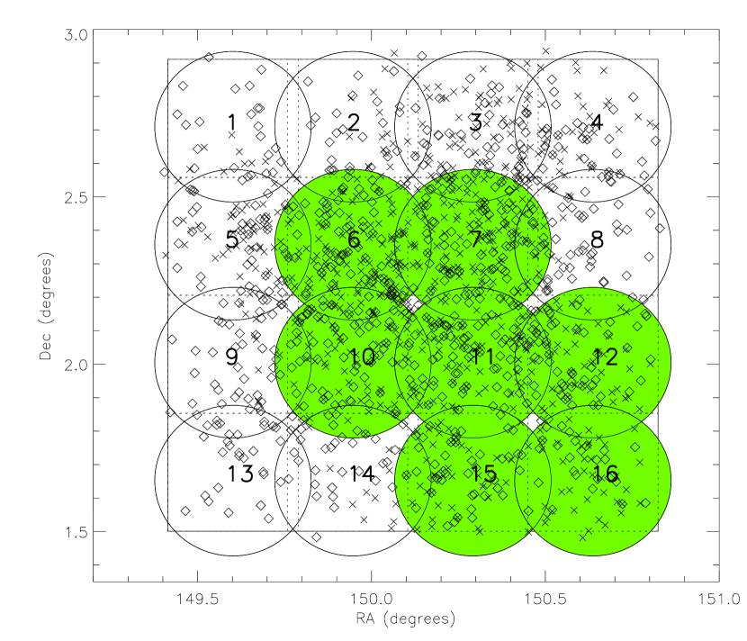
Figure 1.— The sixteen IMACS pointings used to fully cover the COSMOS area. The X-ray targets available for our initial observations are shown as crosses, and radio targets are shown as diamonds. The seven shaded fields were chosen to use the regions of maximum X-ray completeness at the time of our observations, and are the pointings observed for our initial data set.

Figure 2.— The three templates used in our classification and redshift determination scheme. The Type 1 AGN template is the SDSS quasar composite of Vanden Berk et al. (2001), the Type 2 AGN template is the SDSS Type II AGN composite of Zakamska et al. (2003), and the red galaxy template is the composite of the SDSS red galaxy sample (Eisenstein et al., 2001). The wavelength coverages of each template were within the observed wavelength range for the redshift ranges of the different object types in our sample.

Figure 3.— Four example Type 1 AGN spectra. Prominent features are labeled and artifacts are marked by “A.” The three objects at top all have $z_{\rm conf}=1$ and span the range of redshifts sampled by our observations. The bottom spectrum, while an unambiguous Type 1 AGN, has roughly equal likelihood of $z=1.365$ as $z=2.461$ and is therefore assigned $z_{\rm conf}=2$ (its catalog entry is $z=2.461$ because of its broadband colors; see §3.3). Type 1 AGN can be correctly classified even at low signal-to-noise, but may have an ambiguous redshift if only one emission line is present.

Figure 4.— Three Type 2 AGN spectra and one red galaxy type spectrum. Prominent features are labeled and artifacts are marked by “A.” The first two spectra have multiple emission features and are assigned $z_{\rm conf}=1$ redshifts. The second spectrum from the top is an example of how the strong emission lines in a Type 2 AGN allow unambiguous redshifts even if the signal-to-noise is low. The third spectrum has only one emission line that is not an obvious artifact and is assigned $z_{\rm conf}=2$. The bottom spectrum is typical of the red galaxies in our sample and with multiple absorption features is assigned $z_{\rm conf}=1$.

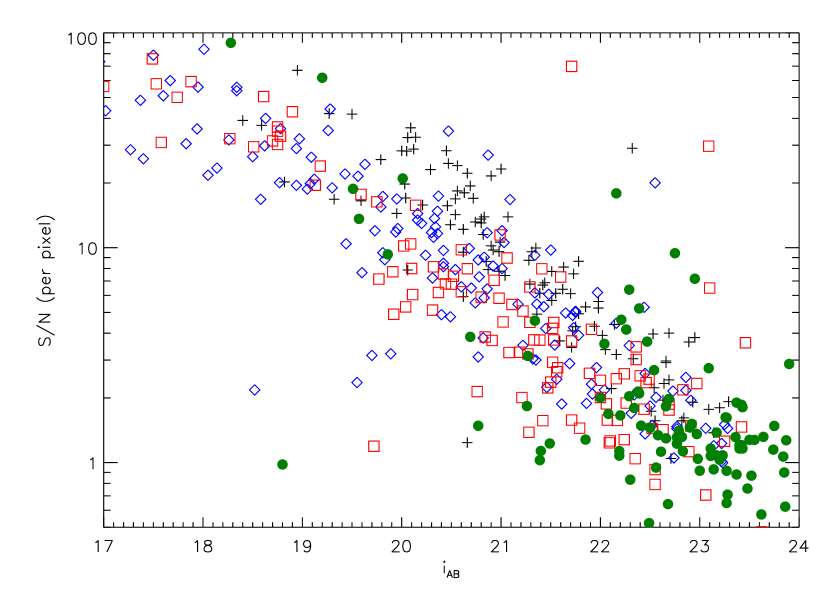
Figure 5.— The measured signal-to-noise of our spectra with their target $i_{\rm AB}$ magnitudes. Black crosses represent Type 1 AGN, blue diamonds are Type 2 AGN, red squares are red galaxies, and filled green circles are unclassified targets. In general, signal-to-noise increases with brighter targets. The outlying objects had poorly machined or misaligned slits or severe contamination from the 0th and 2nd order features of neighboring slits. Our ability to classify targets decreases significantly for S/N$<2.5$ and $i_{\rm AB}<22$.

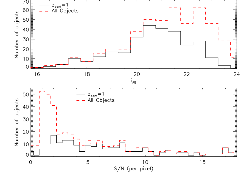
Figure 6.— The distributions of $i_{\rm AB}$ magnitude (top panel) and signal-to-noise (bottom panel) of our sample. The solid lines represent objects with reliable redshifts ($z_{\rm conf}=1$) and the dashed lines represent all objects. A high fraction of spectra with $S/N\gtrsim 2.5$ and $i_{\rm AB}\lesssim 22$ yield reliable redshifts.

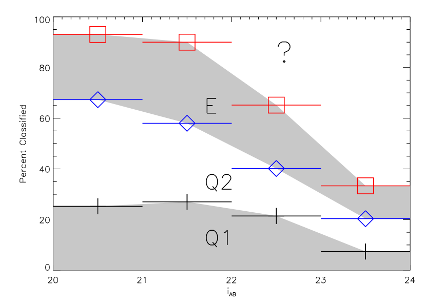
Figure 7.— The completeness of our sample with $i_{\rm AB}$ magnitude, by type. Our completeness to type 1 AGN (the region labeled “Q1”) does not appear to drop off until $i_{\rm AB}>23$, while completeness to type 2 AGN (“Q2”) and red galaxies (“E”) drops for $i_{\rm AB}>22$. The fraction of unclassified objects (labeled “?”) increases significantly after the $21<i_{\rm AB}<22$ bin.

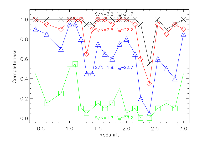
Figure 8.— Our estimated completeness to assigning $z_{\rm conf}=1$ redshifts for Type 1 AGN, as determined by our Monte Carlo simulations. We tested 20 iterations of Gaussian-distributed random errors according to 4 values of signal-to-noise, over 20 redshift bins. Each signal-to-noise corresponds to a $i_{\rm AB}$ magnitude according to Figure 5. The redshift ranges of lowest completeness correspond to the regions in which Mgii and Ciii] are the only lines present for our wavelength coverage.

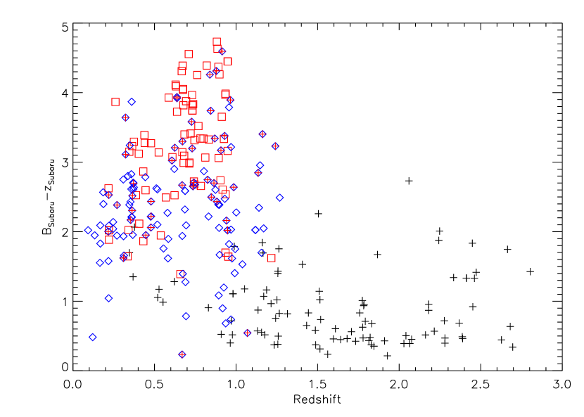
Figure 9.— The Subaru $B-z$ color of our targets with redshift. Black crosses represent Type 1 AGN, blue diamonds are Type 2 AGN, and red squares are red galaxies. Hybrid “q2e” targets with emission lines and red galaxy continua are blue diamonds filled with red. Because our targets have different $B-z$ colors at all redshifts (though especially at $z\sim 1$), we should be able to place constraints on the unclassified targets using their $B$ and $z$ colors.

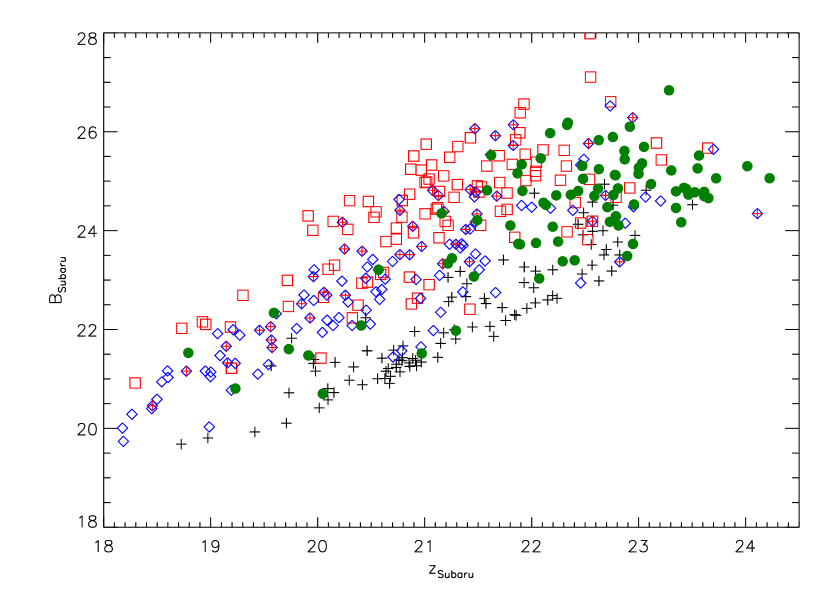
Figure 10.— The distribution of Subaru $B$ and $z$ colors for the Type 1 AGN (black crosses), Type 2 AGN (blue diamonds, with hybrid “q2e” objects filled red), red galaxies (red squares), and unclassified targets (green filled circles). For $z<23$, the colors of our unclassified targets suggest that they are mostly red galaxies or Type 2 AGN. We cannot constrain the $z>23$ unclassified targets as effectively.

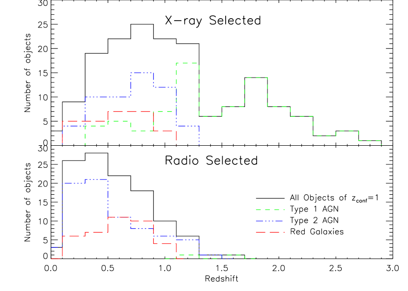
Figure 11.— The distribution of redshifts for X-ray selected and radio selected target identified in our sample. The solid line represents all objects of a given selection method, with the distribution of Type 1 AGN shown by the green short-dashed line, Type 2 AGN by the blue dash-dotted line, and red galaxies by the red long-dashed line. X-ray selected Type 1 AGN dominate the $z\gtrsim 1$ population of our sample. The radio selected distribution has an additional low redshift Type 2 population which is probably dominated by emission line galaxies.

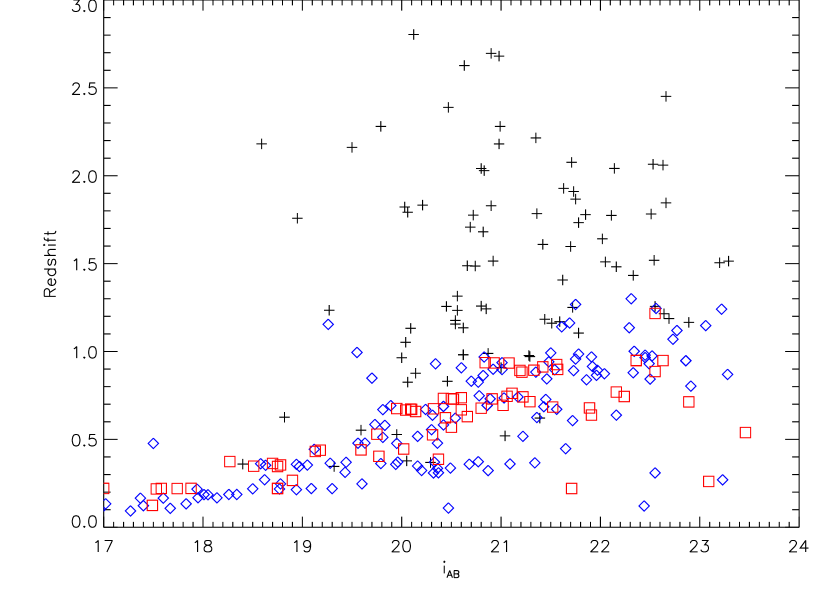
Figure 12.— The relationship between our redshifts and the $i_{\rm AB}$ magnitudes. Type 1 AGN are represented by crosses, Type 2 AGN by the diamonds, and galaxies by the squares. While the Type 2 AGN and red galaxies follow a very similar distribution, the Type 1 AGN are on average significantly more distant and luminous.

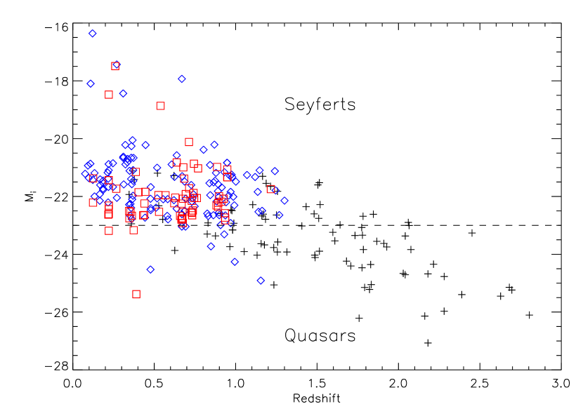
Figure 13.— The absolute $i$-magnitudes with redshifts for our targets. Type 1 AGN are represented by crosses, Type 2 AGN by diamonds, and red galaxies by squares. Our spectroscopic survey is sensitive to a variety of Seyfert and quasar AGN for $z<1.5$.

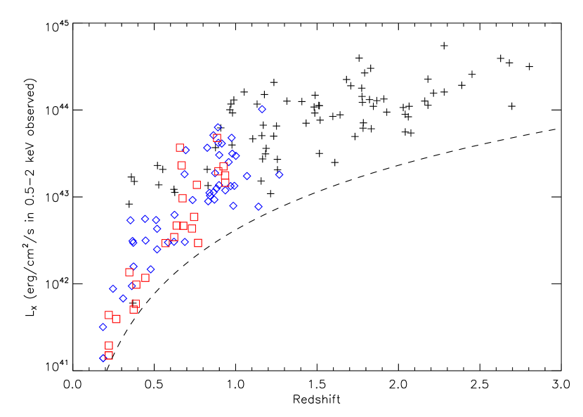
Figure 14.— The X-ray luminosities of our X-ray targets with their redshifts. Type 1 AGN are represented by crosses, Type 2 AGN by diamonds, and red galaxies by squares. The X-ray flux limit of our targets is shown as the dashed line. X-ray luminosities are calculated from the X-ray flux in the observed 0.5-2 keV band.

Table 1COSMOS Observation Details by Field

Field	$t_{\rm exp}$(Jan.)	$t_{\rm exp}$(Feb.)	$n_{\rm targets}$	$n_{\rm X-ray}$	$n_{\rm radio}$	$n(z_{\rm conf}=1)$
6	24840	…	77	44	33	52
7	12720	9000	100	66	34	62
10	13200	21470	68	36	32	31
11	…	16800	73	46	27	45
12	…	17160	65	38	27	32
15	…	13080	43	24	19	33
16	…	14160	40	28	12	27

Table 2COSMOS IMACS AGN catalog (page 1)

Object Name	RA (J2000)	Dec (J2000)	$i_{\rm CFHT}$	S/N	$t_{\rm exp}$	Type	z	$\sigma_{z}$	$z_{\rm conf}$
COSMOS J095859.33+022044.7	149.7472229	2.3457551	18.61	50.51	24840	e	0.37389	0.00002	2
COSMOS J095900.62+022833.3	149.7525635	2.4759071	19.95	16.87	24840	q2	0.47723	0.00007	1
COSMOS J095900.64+021954.4	149.7526398	2.3317800	20.36	14.78	24840	q2	0.33492	0.00001	1
COSMOS J095901.82+021449.6	149.7575989	2.2471199	22.39	2.10	24840	?	-1.00000	-1.00000	?
COSMOS J095902.56+022511.8	149.7606354	2.4199319	21.78	4.92	24840	q1	1.10490	0.00592	1
COSMOS J095902.66+022738.8	149.7610931	2.4607720	20.10	8.00	24840	e	0.67068	0.00034	1
COSMOS J095904.41+020333.8	149.7683563	2.0594010	21.26	1.83	13200	?	-1.00000	-1.00000	?
COSMOS J095906.97+021357.8	149.7790222	2.2327120	21.11	5.44	24840	e	0.76203	0.00052	1
COSMOS J095907.65+020820.9	149.7818756	2.1391280	19.05	18.75	13200	q2e	0.35416	0.00004	1
COSMOS J095908.23+015446.2	149.7842865	1.9128259	21.32	3.04	13200	q2	1.15604	0.00030	2
COSMOS J095908.34+020540.7	149.7847443	2.0946369	17.27	28.58	13200	q2	0.09308	0.00004	1
COSMOS J095908.40+020403.7	149.7849884	2.0677061	17.67	59.98	13200	q2	0.10792	0.00003	1
COSMOS J095908.77+022315.2	149.7865601	2.3875580	23.06	0.71	24840	e	0.91729	0.00432	2
COSMOS J095909.53+021916.5	149.7897339	2.3212631	20.05	28.16	24840	q1	0.37753	0.00005	1
COSMOS J095909.97+022017.7	149.7915649	2.3382571	21.41	7.98	24840	e	0.43187	0.00156	2
COSMOS J095910.02+020509.4	149.7917480	2.0859480	23.87	1.27	13200	?	-1.00000	-1.00000	?

Table 3Breakdown of AGN Candidates

	X-ray Targets		Overlap		Radio Targets
	Total	Example	Total	Example	Total	Example
Total $i_{\rm AB}<24$ sources	800	58	150	10	700	43
Targeted	660	48	-	-	420	28
Classified	500	41	-	-	350	23
Assigned $z_{\rm conf}=1$ Redshifts	390	28	-	-	280	18
Assigned $z_{\rm conf}=2$ Redshifts	80	8	-	-	45	3

References

- Abraham et al. (2004) Abraham, R. G. et al. 2004, AJ, 127, 2455
- Best et al. (2005) Best, P. N., Kauffmann, G., Heckman, T. M., Ivezić, Z. 2005, MNRAS, 362, 9
- Bigelow et al. (1998) Bigelow, B. C., Dressler, A. M., Shectman, S. A., & Epps, H. W. 1998, in Proc. SPIE Vol. 3355, p. 225-231, Optical Astronomical Instrumentation, Sandro D’Odorico; Ed., 225–231
- Brusa et al. (2006) Brusa, M. et al. 2006, ApJS, this volume
- Budavári et al. (2001) Budavári, T. et al. 2001, AJ, 122, 1163
- Eckart et al. (2006) Eckart, M. E., Stern, D., Helfand, D. J., Harrison, F. A., Mao, P. H., & Yost, S. A. 2006, ApJ in press (astro-ph/0603556)
- Eisenstein et al. (2001) Eisenstein, D. J. et al. 2001, AJ, 122, 2267
- Fiore et al. (2003) Fiore et al. 2003, A&A, 409, 79
- Glazebrook & Bland-Hawthorn (2001) Glazebrook, K. & Bland-Hawthorn, J. 2001, PASP, 113, 197
- Hasinger, Miyaji, & Schmidt (2005) Hasinger, G., Miyaji, T. & Schmidt, M. 2005, A&A, 441, 417
- Hasinger et al. (2006) Hasinger, G. et al. 2006, ApJS, this volume
- Impey et al. (2006) Impey, C. D. et al. 2006, ApJS, this volume
- La Franca et al. (2005) La Franca, L. et al. 2005, ApJ, 635, 864
- Lilly et al. (2006) Lilly, S. J. et al. 2006, ApJS, this volume
- Mainieri et al. (2006) Mainieri, V. et al. 2006, ApJS, this volume
- Moustakas & Kennicutt (2005) Moustakas, J. & Kennicutt, R. C. 2005, ApJS, submitted
- Sadler et al. (2002) Sadler, E. M. et al. 2002, MNRAS, 329, 227
- Schinnerer et al. (2006) Schinnerer, E. et al. 2006, ApJS, this volume
- Scoville et al. (2006) Scoville, N. Z. et al. 2006, ApJS, this volume
- Silverman et al. (2005) Silverman, J. D. et al. 2005, ApJ, 618, 123
- Smolcic et al. (2006) Smolcic, V. 2006, in prep.
- Steffen et al. (2003) Steffen, A. T., Barger, A. J., Cowie, L. L, Mushotzky, R. F., & Yang, Y. ApJ, 596, 23
- Sulentic et al. (2000) Sulentic, J. W., Marziani, P., & Dultzin-Hacyan, D. 2000, ARA&A, 38, 521
- Trump et al. (2006) Trump, J. R. et al. 2006, in prep.
- Vanden Berk et al. (2001) Vanden Berk, D. E. et al. 2001, AJ, 122, 549
- York et al. (2000) York, D. G. et al. 2000, AJ, 120, 1579
- Zakamska et al. (2003) Zakamska, N. L. et al. 2003, AJ, 126, 2125