Refining a relativistic, hydrodynamic solver: Admitting ultra-relativistic flows

Abstract

We have undertaken the simulation of hydrodynamic flows with bulk Lorentz factors in the range 10²–10⁶. We discuss the application of an existing relativistic, hydrodynamic primitive-variable recovery algorithm to a study of pulsar winds, and, in particular, the refinement made to admit such ultra-relativistic flows. We show that an iterative quartic root finder breaks down for Lorentz factors above 10² and employ an analytic root finder as a solution. We find that the former, which is known to be robust for Lorentz factors up to at least 50, offers a 24% speed advantage. We demonstrate the existence of a simple diagnostic allowing for a hybrid primitives recovery algorithm that includes an automatic, real-time toggle between the iterative and analytical methods. We further determine the accuracy of the iterative and hybrid algorithms for a comprehensive selection of input parameters and demonstrate the latter’s capability to elucidate the internal structure of ultra-relativistic plasmas. In particular, we discuss simulations showing that the interaction of a light, ultra-relativistic pulsar wind with a slow, dense ambient medium can give rise to asymmetry reminiscent of the Guitar nebula leading to the formation of a relativistic backflow harboring a series of internal shockwaves. The shockwaves provide thermalized energy that is available for the continued inflation of the PWN bubble. In turn, the bubble enhances the asymmetry, thereby providing positive feedback to the backflow.

1 Introduction

Hydrodynamic simulations have been widely used to model a broad range of physical systems. When the velocities involved are a small fraction of the speed of light and gravity is weak, the classical Newtonian approximation to the equations of motion may be used. However, these two conditions are violated for a host of interesting scenarios, including, for example, heavy ion collision systems (Hirano, 2004), relativistic laser systems (Delettrez et al., 2005), and many from astrophysics (Ibanez, 2003, and references therein), that call for a fully relativistic, hydrodynamic (RHD) treatment. The methods of solution of classical hydrodynamic problems have been successfully adapted to those of a RHD nature, albeit giving rise to significant complication; in particular, the physical quantities of a hydrodynamic flow (the rest-frame mass density, $n$, pressure, $p$, and velocity, $v$) are coupled to the conserved quantities (the laboratory-frame mass density, $R$, momentum density, $M$, and energy density, $E$) via the Lorentz transformation. The fact that modern RHD codes typically evolve the conserved quantities necessitates the recovery of the physical quantities (often referred to as the “primitive variables”) from the conserved quantities in order to obtain the flow velocity. Thus, the calculation of the primitives from the conserved variables has become a critical element of modern RHD codes (Martí and Müller, 2003). Indeed, this is an active area of research with significant attention given to the case of general relativistic, magnetohydrodynamic (GRMHD) case (e.g. Noble et al., 2006) and varying equations of state within the context of RMHD (e.g. Mignone and McKinney, 2007) and RHD (e.g. Ryu et al., 2006). This work is concerned with the RHD case for a fixed adiabatic index and so we refer the reader to the above-mentioned papers for a discussion of those studies.

In this paper, we present a method for recovering the primitive variables from the conserved quantities representing special relativistic, hydrodynamic (SRHD) flows with bulk Lorentz factors ($\gamma=(1-v^{2})^{-1/2}$, where $v$ is the bulk flow velocity – the speed of light is normalized to unity throughout this paper) up to 10⁶. We started with a module from an existing SRHD code used to simulate flows with $\gamma\leq$50 as described in Duncan and Hughes (1994). Admitting flows with such ultra-relativistic Lorentz factors as 10⁶ required significant refinement to the method used in the existing code to calculate the flow velocity from the conserved quantities. In particular, such extreme Lorentz factors lead to severe numerical problems such as effectively dividing by zero and subtractive cancellation. In $\S$2, we discuss the formalism of recovering the primitives within the context of the Euler equations. In $\S$3, we elucidate the details of the refinement to this formalism necessitated by ultra-relativistic flows. We present the refined primitives algorithm in $\S$4 and our application in $\S$5. We discuss our results and conclusions in $\S$6 and $\S$7, respectively.

2 Recovering the primitive variables from $R$, $M$, and $E$

In general, recovering the primitives from the conserved quantities reduces to solving a quartic equation, $Q(v)=0$, for the flow velocity in terms of $R$, $M$, and $E$. Implementation typically involves a numerical root finder to recover the velocity via Newton-Raphson iteration which is very efficient and provides robustness because it is straightforward to ensure that the computed velocity is always less than the speed of light. This is a powerful method that is independent of dimensionality and symmetry. The latter point follows directly from the fact that symmetry is manifest only as a source term in the Euler equations and does not enter into the derivation of $Q(v)$ (see the axisymmetric example below). Dimensional generality arises because regardless of the coordinate system, one may always write $M=\sqrt{\sum M_{x_{i}}^{2}}$, where the $M_{x_{i}}$ are the components of the momentum-density vector along the orthogonal coordinates $x_{i}$. In the case of magnetohydrodynamic (MHD) flows, there are, of course, additional considerations. However, non-magnetic (RHD) simulations still have a significant role to play in astrophysics, e.g. extragalactic jets (Hughes, 2005) and pulsar wind nebulae (van der Swaluw et al., 2004).

As an example, consider the case of the axisymmetric, relativistic Euler equations, which we apply to pulsar winds. This type of formalism enjoys diverse application, in both special and general relativistic settings, from 3D simulations of extragalactic jets (Hughes et al., 2002), to theories of the generation of gamma-ray bursts (Zhang et al., 2003) and the collapse of massive stars to neutron stars and black holes (Shibata, 2003). In cylindrical coordinates $\rho$ and $z$, and defining the evolved-variable, flux, and source vectors

$$U = (R,M_{\rho},M_{z},E)^{T}\rm,$$

$$F^{\rho} = (Rv^{\rho},M_{\rho}v^{\rho}+p,M_{z}v^{\rho},(E+p)v^{\rho})^{T}\rm,$$

$$F^{z} = (Rv^{z},M_{\rho}v^{z},M_{z}v^{z}+p,(E+p)v^{z})^{T}\rm,$$

$$S = (0,p/{\rho},0,0)^{T}\rm,$$ (1)

the Euler equations may be written in almost-conservative form as:

$${\partial{U}\over\partial{t}}+{1\over\rho}{\partial\over\partial{\rho}}(\rho F^{\rho})+{\partial\over\partial z}(F^{z}) = S\rm.$$

The pressure is given by the ideal gas equation of state $p=(\Gamma-1)(e-n)$, where $e$ and $\Gamma$ are the rest-frame total energy density and the adiabatic index. Note that the velocity and pressure appear explicitly in the relativistic Euler equations, in addition to the evolved variables, and pressure and rest density are needed for the computation of the wave speeds that form the basis of typical numerical hydrodynamic solvers, such as that due to Godunov (1959). We obtain these values by performing a Lorentz transformation where the rest-frame values are required:

$$R = \gamma n\rm,$$

$$M_{\rho} = \gamma^{2}(e+p)v^{\rho}\rm,$$

$$M_{z} = \gamma^{2}(e+p)v^{z}\rm,$$

$$E = \gamma^{2}(e+p)-p\rm,$$

$$\gamma = (1-v^{2})^{-1/2}\rm,$$ (2)

where $v^{2}=(v^{\rho})^{2}+(v^{z})^{2}$ and $M^{2}$ = $\gamma^{4}(e+p)^{2}[(v^{\rho})^{2}+(v^{z})^{2}]$ = $\gamma^{4}(e+p)^{2}v^{2}$. When the adiabatic index is constant, combining the above equations with the equation of state creates a closed system which yields the following quartic equation for $v$ in terms of $Y\equiv M/E$ and $Z\equiv R/E$:

$$Q(v) = (\Gamma-1)^{2}(Y^{2}+Z^{2})v^{4}-2\Gamma(\Gamma-1)Yv^{3}$$ (3)

$$+ \Bigl{[}\Gamma^{2}+2(\Gamma-1)Y^{2}-(\Gamma-1)^{2}Z^{2}\Bigr{]}v^{2}$$

$$- 2\Gamma Yv+Y^{2}\;=\;0\rm.$$

Component velocities, and the rest-frame total energy and mass densities are then given by:

$$v^{\rho} = {M_{\rho}\over M}v\rm,$$

$$v^{z} = {M_{z}\over M_{\rho}}v^{\rho}\rm,$$

$$e = E-M_{\rho}v^{\rho}-M_{z}v^{z}\rm,$$

$$n = {R\over\gamma}\rm.$$

3 Refinement of the root finder to admit ultra-relativistic flows

A particular implementation of the above has been previously applied to relativistic galactic jets with $\gamma\leq 50$ (Duncan and Hughes, 1994). The ultra-relativistic nature of pulsar winds necessitated an investigation of the behavior of the primitives algorithm upon taking $\gamma>>1$. We found that, beyond $\gamma\sim 10^{2}$, the algorithm suffers a severe degradation in accuracy that worsens with increasing Lorentz factor until complete breakdown occurs due to the failure of the Newton-Raphson iteration process used to calculate the flow velocity.

The problem lies in the shape of the quartic, $Q(v)$, one must solve to calculate the primitive variables. The quartic equation as derived using the velocity as a variable exhibits two roots for typical physical parameters of the flow (see Fig. 1). In general, for $\gamma<10^{2}$, the two roots are sufficiently separated on the velocity axis such that the Newton-Raphson (N-R) iteration method converges to the correct zero very quickly and accurately (for $Y<0.9$ and $Z>10^{-5}$, corresponding to $\gamma<2$, the roots approach each other sufficiently such that the incorrect root is selected; see $\S$4.3). In fact, N-R iteration can be so efficient that it is more desirable to use this method than it is to calculate the roots of the quartic analytically (see $\S$4.2). However, as the Lorentz factor of the flow increases, the roots move progressively closer together and the minimum in $Q(v)$ approaches zero. Eventually, the minimum equals zero to machine accuracy which causes $dQ/dv=0$ to machine accuracy resulting in a divide by zero and the Newton-Raphson method fails (see Fig. 2).

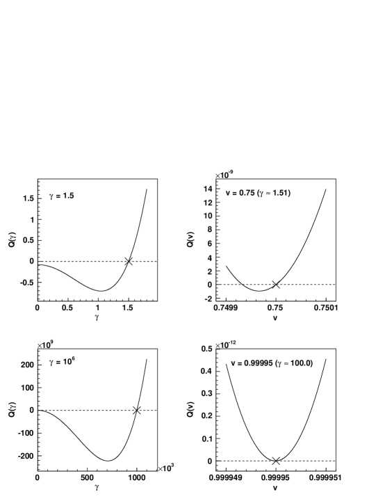
Figure 1: The left-hand plots show the shape of the Lorentz factor quartic over a run of Lorentz factors for a mildly relativistic flow ($\gamma_{o}=1.5$) and an ultra-relativistic flow ($\gamma_{o}=10^{6}$). The right-side plots show the shape of the velocity quartic over a run of velocity for a mildly relativistic flow ($\gamma_{o}\approx 1.5$) and a highly (but not ultra) relativistic flow ($\gamma_{o}\approx 10^{2}$). The crosses mark the location of the physical root. From the plot in the lower right, one can see the onset of the zero derivative problem as the roots are not distinguishable from each other or the local minimum even on a scale of 10^-13, which begins to encroach on the limit of 8-byte accuracy.

A simple and highly effective solution (see $\S$4.3 for details) is to rewrite the velocity quartic, $Q(v)$ (Eqn. 3), in terms of the Lorentz factor (i.e. make the substitution $v^{2}=1-\gamma^{-2}$) to obtain the quartic equation in $\gamma$ (recall $Y\equiv M/E$ and $Z\equiv R/E$):

$$Q(\gamma) = \Gamma^{2}(1-Y^{2})\gamma^{4}-2\Gamma(\Gamma-1)Z\gamma^{3}$$ (4)

$$+ \Bigl{[}2\Gamma(\Gamma-1)Y^{2}+(\Gamma-1)^{2}Z^{2}-\Gamma^{2}\Bigr{]}\gamma^{2}$$

$$+ 2\Gamma(\Gamma-1)Z\gamma-(\Gamma-1)^{2}(Y^{2}+Z^{2})\;=\;0\rm.$$

As Fig. 1 exemplifies, $Q(\gamma)$ exhibits a single root for the physical range $\gamma\geq$ 1. However, Newton-Raphson iteration also fails in this case at high Lorentz factors because of the steepness of the rise in $Q(\gamma)$ through the root. Thus, we are forced to use an analytical method of solving a quartic. Below, we discuss our implementation.

3.1 Solving a quartic equation

We use the prescription due to Bronshtein and Semendyayev (1997) in order to analytically solve for the roots of a quartic. We chose this method because it provides equations for the roots of the quartic that are the most amenable (of the methods surveyed) to integration into a computational environment. In order to provide a complete picture of our method, which includes steps not found in Bronshtein and Semendyayev (1997), we reproduce some sections of that text. We procede as follows.

Given a quartic equation in $x$:

$$a_{4}x^{4}+a_{3}x^{3}+a_{2}x^{2}+a_{1}x+a_{0}=0,\;a_{n}\in\Re,\;a_{4}\neq 0\rm,$$ (5)

normalizing the equation (dividing by $a_{4}$) and making the substitution $y=x+\frac{a_{3}}{4a_{4}}$ results in the reduced form:

$$y^{4}+Py^{2}+Qy+R = 0\rm,$$

where, defining $\tilde{a}_{n}\equiv a_{n}/a_{4}$:

$$P \equiv -\frac{3}{8}\tilde{a}_{3}^{2}+\tilde{a}_{2}\rm,$$

$$Q \equiv \left(\frac{\tilde{a}_{3}}{2}\right)^{3}-\left(\frac{\tilde{a}_{3}}{2}\right)\tilde{a}_{2}+\tilde{a}_{1}\rm,$$

$$\ R \equiv -3\left(\frac{\tilde{a}_{3}}{4}\right)^{4}+\left(\frac{\tilde{a}_{3}}{4}\right)^{2}\tilde{a}_{2}-\left(\frac{\tilde{a}_{3}}{4}\right)\tilde{a}_{1}+\tilde{a}_{0}\rm.$$

These coefficients allow the definition of the cubic resolvent:

$$u^{3}+2Pu^{2}+(P^{2}-4R)u-Q^{2}=0\rm,$$ (6)

upon whose solutions the solutions of the original quartic (Eqn. 5) depend. The product of the solutions of the cubic resolvent is $u_{1}u_{2}u_{3}=Q^{2}$ (Vieta’s theorem), which clearly must be positive. The characteristics of the quartic’s roots depend on the nature of the roots of the cubic resolvent (see Tab. LABEL:charqsolns).

Table 1: The dependence of the solutions to the parent quartic on the solutions to the cubic resolvent.

Solutions of the cubic resolvent	Solutions of the quartic equation
all real and positive	all real
all real, one positive	two complex conjugate (cc) pairs
one real, one cc pair	two real, one cc pair

Given the solutions of the cubic resolvent $u_{1}$, $u_{2}$, and $u_{3}$, the solutions of the quartic (Eqn. 5) are

$$x_{1} = \frac{1}{2}(\sqrt{u_{1}}+\sqrt{u_{2}}+\sqrt{u_{3}})-\frac{a_{3}}{4a_{4}}\rm,$$

$$x_{2} = \frac{1}{2}(\sqrt{u_{1}}-\sqrt{u_{2}}-\sqrt{u_{3}})-\frac{a_{3}}{4a_{4}}\rm,$$

$$x_{3} = \frac{1}{2}(-\sqrt{u_{1}}+\sqrt{u_{2}}-\sqrt{u_{3}})-\frac{a_{3}}{4a_{4}}\rm,$$

$$x_{4} = \frac{1}{2}(-\sqrt{u_{1}}-\sqrt{u_{2}}+\sqrt{u_{3}})-\frac{a_{3}}{4a_{4}}\rm.$$ (7)

3.2 Solving a cubic equation

The equations of the previous section reduce the problem of solving a quartic equation to that of solving a cubic equation (i.e. the cubic resolvent of Eqn. 6).

Once again following Bronshtein and Semendyayev (1997) (note the similarity to the method in the previous section), given a cubic equation:

$$b_{3}u^{3}+b_{2}u^{2}+b_{1}u+b_{0}=0,\;b_{n}\in\Re,\;b_{3}\neq 0\rm,$$ (8)

normalizing the equation and making the substitution $v=u+b_{2}/3b_{3}$ results in the reduced form:

$$v^{3}+pv+q = 0\rm,$$

where, defining $\tilde{b}_{n}\equiv b_{n}/b_{3}$:

$$p \equiv -\frac{1}{3}\tilde{b}_{2}^{2}+\tilde{b}_{1}\rm,$$

$$q \equiv 2\left(\frac{\tilde{b}_{2}}{3}\right)^{3}-\left(\frac{\tilde{b}_{2}}{3}\right)\tilde{b}_{1}+\tilde{b}_{0}\rm.$$

These coefficients allow the definition of the discriminant:

$$D \equiv \left(\frac{p}{3}\right)^{3}+\left(\frac{q}{2}\right)^{2}\rm,$$ (9)

upon which the characteristics of the solutions of the cubic equation depend (see Tab. LABEL:charcsolns).

Table 2: The dependence of the solutions of a cubic equation on the sign of the discriminant (assuming a real variable).

D	Solutions of the cubic equation
$positive$	one real, one complex conjugate pair
$negative$	all real and distinct
$=0$	all real, two (one, if $p=q=0$) distinct

Given $p$, $q$, and $D$, Cardando’s formula for the reduced form of the cubic leads to the solutions of the original cubic (Eqn. 8):

$$u_{1} = s+t-\frac{b_{2}}{3b_{3}}\rm,$$

$$u_{2} = -\frac{1}{2}(s+t)-\frac{b_{2}}{3b_{3}}+i\frac{\sqrt{3}}{2}(s-t)\rm,$$

$$u_{3} = -\frac{1}{2}(s+t)-\frac{b_{2}}{3b_{3}}-i\frac{\sqrt{3}}{2}(s-t)\rm,$$ (10)

where:

$$s \equiv \sqrt[3]{-\frac{1}{2}q+\sqrt{D}}\rm,$$

$$t \equiv \sqrt[3]{-\frac{1}{2}q-\sqrt{D}}\rm,$$

$$i \equiv \sqrt{-1}\rm.$$

If $D\leq 0$, the the cubic has three real roots, subject to the following two subcases, and the four real roots of the quartic follow directly from Eqn. 7. If $D=0$, then $s=t$ and the cubic has three real solutions that follow directly from Eqn. 10 from which one can see that two are degenerate. If $D<0$, the cubic has three distinct real roots. Obtaining these solutions via Eqn. 10 requires intermediate complex arithmetic. However, this may be circumvented by making the substitutions:

$$r = \sqrt{-\left(\frac{p}{3}\right)^{3}}$$

$$\cos(\phi) = -\frac{q}{2r}\rm,$$

in which case the solutions of the cubic (Eqn. 8) are:

$$u_{1} = 2\sqrt[3]{r}\cos\left(\frac{\phi}{3}\right)-\frac{b_{2}}{3b_{3}}\rm,$$

$$u_{2} = 2\sqrt[3]{r}\cos\left(\frac{\phi+2\pi}{3}\right)-\frac{b_{2}}{3b_{3}}\rm,$$

$$u_{3} = 2\sqrt[3]{r}\cos\left(\frac{\phi+4\pi}{3}\right)-\frac{b_{2}}{3b_{3}}\rm.$$ (11)

If $D>0$, then the cubic has one real root and a pair of complex conjugate roots and the quartic has two real roots and a pair of complex conjugate roots (see Tab. LABEL:charqsolns). Finding the roots of the quartic involves intermediate complex arithmetic which may be circumvented as follows. Defining:

$$R \equiv -\frac{1}{2}(s+t)-\frac{b_{2}}{3b_{3}}\rm,$$

$$C \equiv \frac{\sqrt{3}}{2}(s-t)\rm,$$

Eqn. 10 may be rewritten as:

$$u_{1} = s+t-\frac{b_{2}}{3b_{3}}\rm,$$

$$u_{2} = R+iC\rm,$$

$$u_{3} = R-iC\rm.$$

Next, we have $u_{2,3}=\sqrt{R^{2}+C^{2}}e^{\pm iC/R}$. We then obtain the roots of the quartic from Eqn. 7:

$$x_{1,2} = \frac{\sqrt{u_{1}}}{2}-\frac{a_{3}}{4a_{4}}\pm\sqrt[4]{R^{2}+C^{2}}\cos\left({\frac{C}{2R}}\right)\rm,$$

$$x_{3,4} = \frac{-\sqrt{u_{1}}}{2}-\frac{a_{3}}{4a_{4}}\pm i\sqrt[4]{R^{2}+C^{2}}\sin\left({\frac{C}{2R}}\right)\rm.$$ (12)

Note that $x_{1}$ and $x_{2}$ are the two real solutions.

4 The refined primitives algorithm

Using the method above we created a SRHD primitive algorithm called “REST_ FRAME”. Given the speed advantage of the iterative root finder (see $\S$4.2), it a desirable choice over the analytical method within its regime of applicability, i.e. for low Lorentz factors. As Fig. 2 shows, the iterative root finder is accurate to order 10^-4 (see $\S$4.3) for a sizable region of parameter space including all $R/E$ above the diagonal line between the points (0, $-7$) & (9, 0) in the $\log(R/E)$ vs. $-\log(1-M/E)$ plane (i.e. for $\log(R/E)\geq-(7/9)\times\log(1-M/E)-7$). Therefore, for a given $M/E$ and $R/E$, we check if this inequality is true; if (not) so, we call the (analytical) iterative root finder (see $\S$4.1).

4.1 Pseudo-code

REST_FRAME calculates the primitive variables given the conservative variables and the adiabatic index as represented in the following pseudo-code (note this is a 2D example):

PROCEDURE REST_FRAME
       RECEIVED FROM PARENT PROGRAM: $Y$, $Z$
       RETURNED TO PARENT PROGRAM: $\gamma$, $v$, $C$
Comment: recall $Y\equiv M/E$ and $Z\equiv R/E$
Comment: $C$ is returned $<0$ for code failures
       GLOBAL VARIABLE: $\Gamma$
       SET VALUE OF $m_{underflow}$
       SET VALUE OF $v_{tol}$
Comment: determines iterative method velocity accuracy
Comment: we set $v_{tol}$ = 10^-8, 10^-10, 10^-12, 10^-14
Comment: for $-\log(1-Y)<8.3$, $<10.3$, $<12.3$, otherwise, respectively
       SET $M$ = $\sqrt{M_{x}^{2}+M_{y}^{2}}$
       IF $M<m_{underflow}$ THEN
              $v$ = 0, $\gamma$ = 1
Comment: avoids code failure if $v$ is numerically zero
       ELSE
              TEST FOR UNPHYSICAL PARAMETERS
              IF PASSED, SET $C$ NEGATIVE AND RETURN
              IF $\log(Z)\geq-(7/9)\times\log(1-Y)-7$, THEN
Comment: check to see if input parameters are within the acceptable
Comment: accuracy region of the iterative routine
                     CALL ITERATIVE_QUARTIC($Y,Z,v_{tol},v$,$C$)
Comment: updates $v_{n-1}$ to $v_{n}$ using $n$ cycles of Newton-Raphson iteration
Comment: returns $v$ = $v_{n}$ when $|v_{n}-v_{n-1}|$ $\leq$ $v_{tol}$
                     IF $C<0$, THEN
Comment: this means the iteration failed to converge
                            RETURN
                     ELSE
                            $\gamma$ = $\sqrt{\frac{1}{1-v^{2}}}$
                     END IF
              ELSE
                     CALL ANALYTICAL_QUARTIC($Y,Z,\gamma$)
Comment: calculates $\gamma$ using analytical solution – see below
                     $v$ = $\sqrt{1-\frac{1}{\gamma^{2}}}$
              END IF
       END IF
       END PROCEDURE REST_FRAME

PROCEDURE ANALYTICAL_QUARTIC
Comment: see $\S$3.1 for equations
       RECEIVED FROM PARENT PROGRAM: $Y,Z$
       RETURNED TO PARENT PROGRAM: $\gamma$
       GLOBAL VARIABLE: $\Gamma$
       $\tilde{a}_{3}$ = $2\Gamma(\Gamma-1)Z(Y^{-2}+1)$
       $\tilde{a}_{2}$ = $(\Gamma^{2}-2\Gamma(\Gamma-1)Y^{2}-(\Gamma-1)^{2}Z^{2})(Y^{-2}+1)$
       $\tilde{a}_{1}$ = $-a_{3}$
       $\tilde{a}_{0}$ = $(\Gamma-1)^{2}(Y^{2}+Z^{2})(Y^{-2}+1)$
       $\tilde{a}_{4}$ = $1+Y^{2}-a_{0}-a_{2}$
Comment: coefficients recast to counter subtractive cancellation – see $\S$4.3
       NORMALIZE COEFFICIENTS TO $a_{4}$
Comment: e.g., $a_{3N}$ = $a_{3}/a_{4}$
       CALCULATE CUBIC RESOLVENT COEFFICIENTS
       CALCULATE DISCRIMINANT, $D$
       IF $D\leq$0 THEN
              WRITE ERROR MESSAGE AND STOP
Comment: exploration suggests $D\leq 0$ is unphysical but formal proof is elusive
Comment: thus, we leave $D\leq 0$ uncoded with a error flag just in case
       ELSE
Comment: $D>0$ $\Rightarrow$ $Q(\gamma)$ has 2 real roots (see Tab. LABEL:charqsolns & LABEL:charcsolns)
               CALCULATE ROOTS OF CUBIC RESOLVENT
Comment: the cubic has one real root and a pair of complex conjugate roots
               IF REAL ROOT $<0$, SET REAL ROOT = 0
Comment: the real root cannot be less than zero analytically
Comment: numerically, however, it can have a very small negative value
               CALCULATE THE TWO REAL ROOTS OF THE QUARTIC
               TEST FOR TWO OR NO PHYSICAL ROOTS
               IF PASSED, WRITE ERROR MESSAGE, AND RETURN
               IF FAILED, SET $\gamma$ = PHYSICAL ROOT
       END IF
       END PROCEDURE ANALYTICAL_QUARTIC

4.2 Code timing

Using the Intel Fortran library function CPU_TIME, we calculated the CPU time required to execute 5$\times$10⁷ calls to REST_FRAME for $Y$ = 0.9975 & $Z$ = 1$\times 10^{-4}$ ($\gamma\sim$10) using the Newton-Raphson iterative method with $Q(v)$ and 8-byte arithmetic, and the analytical method with $Q(\gamma)$ and both 8-byte & 16-byte arithmetic (we investigated the use of 16-byte arithmetic due to an issue with subtractive cancellation – see $\S$4.3). The CPU time for each of these scenarios was 29.5, 36.5 (averaged over ten runs and rounded to the nearest half second), and $\sim$11650 seconds (one run only), respectively. This indicates that while using the 8-byte analytical method is satisfactory, it is advantageous to use the iterative method when Lorentz factors are sufficiently low, and that the use of 16-byte arithmetic is a nonviable option. This result is not surprising as the accuracy of Newton-Raphson iteration improves by approximately one decimal place per iterative step (Duncan and Hughes, 1994) and the relative inefficiency of 16-byte arithmetic is a known issue (e.g. Perret-Gallix, 2006).

4.3 Solver Accuracy

The input parameters for our primitives algorithm are the ratios of the laboratory-frame momentum and mass densities to the laboratory-frame energy density (recall $Y\equiv M/E$ and $Z\equiv R/E$) both of which must be less than unity in order for solutions of Eqn. 2 to exist. In addition, the condition $Y^{2}+Z^{2}<1$ must be met. Along with the fact that $Y$ and $Z$ must also be positive, this defines the comprehensive and physical input parameter space to be $0<Y,Z<1$ such that $Y^{2}+Z^{2}<1$ (we identify a particular region of parameter space applicable to pulsar winds in the next section). We tested the accuracy of our iterative and hybrid primitives algorithms within this space as follows.

First, as we are most interested in light, highly relativistic flows (i.e. $Z$ small and $Y$ close to unity), to define the accuracy-search space we elected to use the quantities $-\log(1-Y)$, which for values greater than unity gives $0.9<Y<1$, and $\log(Z)$, which for values less than negative unity gives $Z\ll 1$. We selected $0<-\log(1-Y)<13$ and $-13<\log(Z)<0$ corresponding to Lorentz factors ($\gamma$) between 1 and $2\times 10^{6}$. We chose a range with a maximal $\gamma$ slightly above $1\times 10^{6}$ in order to completely bound the pulsar wind nebula parameter space defined in the next section.

Choosing a relativistic equation of state $\Gamma$= 4/3 and using 1300 points for both $-\log(1-Y)$ and $\log(Z)$, we tested the accuracy of REST_FRAME by passing it $Y$ and $Z$, choosing $E=1$, and using the returned primitive quantities to derive the calculated energy density $Ec$, and calculating the difference $|1-Ec/E|\equiv\delta E/E$. We chose this estimate of the error because $\delta E/E\sim\delta\gamma/\gamma$ and $\delta\gamma/\gamma$ is tied to the accuracy of the numerical, hydrodynamic technique (see the final paragraph in this section).

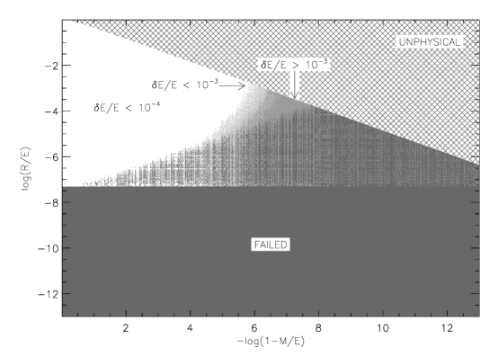
Figure 2: The accuracy (estimated as $\delta E/E$) of the Newton-Raphson (N-R) iterative primitives algorithm where white, light grey, medium grey, dark grey, and hatched regions correspond, respectively, to an accuracy of order at least 10^-4, at least 10^-3, worse than 10^-3, failure, and unphysical input ($R^{2}/E^{2}\geq 1-M^{2}/E^{2}$). Note that the Lorentz factor varies from order 1 at the far left to order 10⁶ at the far right. There is a sizable white region representing $M/E<0.999999$ ($\gamma<500$) and $R/E>5\times 10^{-8}$ within which accuracy is generally significantly better than 10^-4. N-R iteration is unreliable due to sporadic failures for all $M/E$ and $R/E$ such that $R/E<5\times 10^{-8}$ and for an ever increasing fraction of $R/E>5\times 10^{-8}$ as $M/E$ increases until accuracy becomes unacceptable or the code fails outright for $M/E$ and $R/E$ such that $M/E>0.999999$. Failures are due to divide by zero (see §3) or nonconvergence within a reasonable number of iterations.

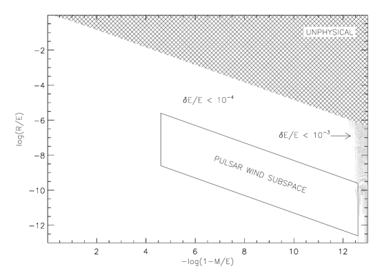
Figure 3: The accuracy (estimated as $\delta E/E$) of the hybrid primitives algorithm where white, light grey, and hatched regions correspond, respectively, to an accuracy of order at least 10^-4, at least 10^-3, and nonphysical input ($R^{2}/E^{2}\geq 1-M^{2}/E^{2}$). Note that the Lorentz factor varies from order 1 at the far left to order 10⁶ at the far right. The space between the parallel lines represents PWNe input parameter space. The accuracy degradation at the extreme right is due to subtractive cancellation in the 4^th-order coefficient of the Lorentz-factor quartic as $M/E\rightarrow$1.

Our results for the Newton-Raphson (N-R) and hybrid methods are given in Figs. 2 & 3 which show where the accuracy is of order at least 10^-4, at least 10^-3, worse than 10^-3, failure, and unphysical input ($Z^{2}\geq 1-Y^{2}$), respectively. We chose an accuracy of order 10^-4 as the upper cutoff because N-R iteration returns accuracies on this order for $\gamma<50$ and relativistic, hydrodynamic simulations of galactic jets by Duncan and Hughes (1994) produced robust results for Lorentz factors of at least 50 using N-R iteration. An additional result of interest is that the ultra-relativistic approximation for $v$ (i.e. taking $R=0$ thereby reducing $Q(v)=0$ to a quadratic equation) manages an accuracy of at least 10^-4 for a large portion of the physical $Y-Z$ plane (see Fig. 4).

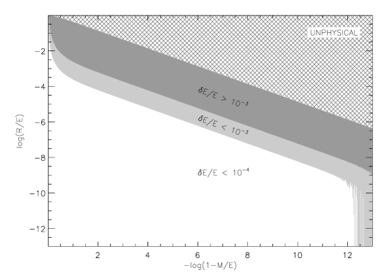
Figure 4: The accuracy (estimated as $\delta E/E$) of the ultra-relativistic approximation of the flow velocity where white, light grey, medium grey, and hatched regions correspond to an accuracy of order at least 10^-4, at least 10^-3, worse than 10^-3, and unphysical input ($R^{2}/E^{2}\geq 1-M^{2}/E^{2}$), respectively. Note that the Lorentz factor varies from order 1 at the far left to order 10⁶ at the far right. The accuracy degradation at the extreme right is due to the fact that the fractional error in the Lorentz factor is proportional to the fractional error in the velocity divided by $1-v^{2}$ which diverges as $v\rightarrow$1.

Fig. 2 shows the accuracy of the N-R iterative method. There are several noteworthy features. First is the presence of a sizable region corresponding to $\gamma<500$ within which accuracy is generally significantly better than 10^-4. Second is that N-R iteration is unreliable due to sporadic failures for increasing Lorentz factors until accuracy becomes unacceptable or the code fails outright due to divide by zero (see §3) or non-convergence within a reasonable number of iterations. In addition, though N-R iteration has been widely established as the primitives recovery method of choice for flows with Lorentz factors less than order 10², we found that for a subset of parameters, corresponding to $\gamma<2$, our N-R algorithm suffered an unacceptable degradation in accuracy. The key to this problem lies in the how the flow velocity ($v$) is initially estimated for the first iterative cycle as follows:

1. The established approach (Duncan and Hughes, 1994; Schneider et al., 1993) is to bracket $v$ with

   $$v_{max} = min(1,Y+\delta)\rm,$$

   $$v_{min} = \frac{\Gamma-\sqrt{\Gamma^{2}-4(\Gamma-1)Y^{2}}}{2Y(\Gamma-1)}\rm,$$ (13)

   where $\delta\sim 10^{-6}$ and $v_{min}$ is derived by taking the ultra-relativistic limit (i.e. $R=0$)

2. The initial velocity is then $v_{i}=(v_{min}+v_{max})/2+\eta$, where $\eta=(1-Z)(v_{min}-v_{max})$ for $v_{max}>\epsilon$ and $\eta=0$ otherwise ($\epsilon$ order 10^-9)

3. This method fails due to selection of the incorrect root when the roots converge.

4. Thus, we make a simpler initial estimate of $v_{i}=v_{max}$, which guarantees that $v_{i}$ is “uphill” from $v$ for all physical $Y-Z$ space and that N-R iteration converges on $v$.

Fig. 3 shows that our hybrid algorithm REST_FRAME is accurate to at least 10^-4 for all but a smattering of the highest Lorentz factors. In fact, it is significantly more accurate over the majority of the physical portion of the $Y-Z$ plane. The space between the parallel lines represents the PWN input parameters discussed in the next section. We find that multiplying $Q(\gamma)$ by $(Y^{2}-Y^{-2})$ and rewriting the new $a_{4}$ ($\tilde{a}_{4}$) in terms of the new $a_{2}$ ($\tilde{a}_{2}$) and new $a_{0}$ ($\tilde{a}_{0}$), e.g. $\tilde{a}_{4}=1+Y^{2}-\tilde{a}_{0}-\tilde{a}_{2}$, improves the accuracy somewhat, but does not entirely mitigate the problem. The issue of accuracy loss at large Lorentz factors in 8-byte primitives algorithms is a known issue (e.g. Noble, 2003) for which we know of no complete 8-byte solution. Employing 16-byte arithmetic provides spectacular accuracy, but introduces an unacceptable increase in run time (see $\S$4.2).

The issue of what constitutes an acceptable error in the calculated Lorentz factor is decided by the fact that a fractional error in $\gamma$ translates to the same fractional error in $p$ and $n$ which are needed to calculate the wave speeds that form the basis of the numerical, hydrodynamic technique, a Godunov scheme (Godunov, 1959) which approximates the solution to the local Riemann problem by employing an estimate of the wave speeds. We do not know a priori how accurate this estimate needs to be, and so procede with 8-byte simulations of pulsar winds with the expectation of using shock-tube tests (Thompson, 1986) to validate the accuracy of the computation of well-defined flow structures as we approach the highest Lorentz factors. It is also noteworthy that while $\gamma$ = 10⁶ is the canonical bulk Lorentz factor for pulsar winds, $\gamma$ = 10⁴ and 10⁵ are still in the ultra-relativistic regime, and it may very well prove to be that these Lorentz factors are high enough to elucidate the general ultra-relativistic, hydrodynamic features of such a system. The hybrid algorithm achieves accuracies of at least 10^-6 for $\gamma\sim 10^{5}$, which is safely in the acceptable accuracy regime.

5 Application to Bow-shock Pulsar Wind Nebulae

At the end of a massive star’s life, the collapse of its core to a compact object, i.e. a neutron star or black hole, drives a shockwave into its outer layers, thereby heating and ejecting them into the interstellar medium (ISM) in a supernova (SN) explosion. Subsequently, the shockwave overtakes the ejecta, expanding into the ISM, and forming a supernova remnant (SNR). Typically, a SN releases $\sim$10⁵¹ erg of mechanical energy that drives expansion of the SNR, sweeping up ISM material, heating it to X-ray temperatures and infusing it with fusion products beyond lithium.

In a subclass of SNRs, for progenitor masses between 10 and 25 solar masses (e.g. Heger et al., 2003), the compact object formed in the SN explosion is a rapidly-spinning, highly-magnetized neutron star surrounded by a magnetosphere of charged particles. The combination of the rotation and the magnetic field gives rise to extremely powerful electric fields that accelerate charged particles to high velocities. The magnetic field interacts with the charged particles resulting in the spin-down of the neutron star, and the release of spin-down energy. A relatively small fraction of this energy is converted into beamed emission, manifest as an apparent pulse if the neutron star’s rotation sweeps the beam across the Earth, leading to the designation “pulsar”. The bulk of the spin-down energy is converted into a pulsar wind (Michel, 1969) which is terminated at a strong shock, downstream of which the flow is indistinguishable from being spherically symmetric (e.g. Chatterjee and Cordes, 2002). The wind particles interact with the magnetic field causing them to emit synchrotron radiation, forming a pulsar wind nebula (PWN). The Crab Nebula, formed in the SN explosion of 1054 CE, is the canonical object of this type. The Crab exhibits pulsations from the radio, all the way up to X-rays, and is a prodigious source of $\gamma$-rays.

The wind in the immediate vicinity of the pulsar is a diffuse, relativistic gas unlikely to be directly observable. However, the classic structure of forward and reverse shocks separated by a contact surface (Weaver et al., 1977) arises from the wind interaction with the SNR or ISM. A probe of this interaction is provided by optical emission from the swept-up ambient ISM, thermal X-ray emission from the SNR and/or the shocked ISM, and X-ray synchrotron emission from the shocked wind. Furthermore, the high space velocity that is typical of pulsars (Cordes and Chernoff, 1998) implies an asymmetric ram pressure on the pulsar wind from the denser ambient medium. The details of the morphology and of the distribution of the density, pressure, and velocity within the PWN depends upon the density, speed, momentum, and energy flux of the pulsar wind. Thus, comparison of PWN simulations with observational data can provide an unparalleled method for investigating pulsar winds and, hence, how the surrounding medium taps the rotational energy of the pulsar.

Pacini and Salvati (1973) and Rees and Gunn (1974) pioneered the basic model of PWNe; a model further developed by Kennel and Coroniti (1984a, b) and Emmering and Chevalier (1987). Gaensler and Slane (2006) and Bucciantini (2008) are excellent reviews on observational and theoretical studies of PWNe, respectively. For a number of reasons, a detailed, quantitative study of PWNe is now particularly timely. First, there is a cornucopia of high-quality data from space-born observatories such as the $Chandra$ X-ray Observatory and XMM-Newton. Second, the total energy radiated by PWNe accounts for only a small fraction of the spin-down energy, leaving a large energy reservoir available for interaction with the SNR and acceleration of ions, the partitioning of which is not well understood.

Efforts to model PWNe span three decades (with seminal papers Rees and Gunn, 1974; Kennel and Coroniti, 1984a, b; Emmering and Chevalier, 1987). While the case for a non-isotropic pulsar wind energy flux has long been made (Michel, 1973), it has only been recently that a theoretical explanation of the mechanism behind the jet/torus structure interior to the termination shock has been put forward, and that the predictions of Michel (1973) have been confirmed (Bucciantini, 2008). In particular, Bucciantini (2008) highlighted that a detailed description has been made possible by the increase in the efficiency and robustness of relativistic, numerical MHD codes stemming from the work of Komissarov (1999), Del Zanna et al. (2003) and Gammie et al. (2003). Simulations by Del Zanna et al. (2004) indicate that where jet formation in PWNe takes place is tied to where the magnetic field attains equipartition, at which point the magnetic filed can no longer be compressed. If this happens close to the termination shock, then, due to the mildly relativistic nature of the post-shock flow, hoop stresses can become efficient and most of the flow is diverted back toward the axis and collimated. The magnitude of the magnetization is key: if it is too small, the equipartition is reached outside the nebula, hoop stresses remain inefficient, and no collimation is produced.

Other modeling, for example, that presented herein, is concerned with the global structure of PWNe. The enormous acceleration of the wind at the termination shock smears out asymmetries leaving an essentially spherically symmetric shocked flow to produce large scale PWN features. In particular, Bucciantini et al. (2005) and Vigelius et al. (2007) are two recent examples of simulations addressing the structures that arise in bow-shock PWNe (see below). Bucciantini et al. (2005) were the first to apply a fully-relativistic MHD code (Del Zanna et al., 2003; Del Zanna and Bucciantini, 2002), and, for an axisymmetric geometry, obtained a relativistic backflow behind the pulsar, as predicted by Wang et al. (1993) for PSR1929+10. However, the wind Lorentz factor and pulsar velocity were 10 and 9000 km s^-1, respectively, which are far from the typical values of 10⁶ and 500 km s^-1 (indeed, the Guitar pulsar, the fastest known, has a transverse velocity of $\sim$1700 km s^-1). In addition, the paper does not address the “bubble” in the Guitar (see Fig. 5). Vigelius et al. (2007) performed non-relativistic, hydrodynamic simulations with a relaxation to cylindrical symmetry. The full 3-D FLASH code (Fryxell et al., 2000) was employed and an anisotropic pulsar wind, cooling of the shocked ISM, ISM density gradients, and ISM walls were considered. While the authors employed a realistic pulsar velocity of 400 km s^-1, the non-relativistic nature of the simulations limited the Lorentz factor to order unity. In this section, we present fully-relativistic, axisymmetric, hydrodynamic simulations of bow-shock PWNe for a realistic pulsar velocity and wind Lorentz factor. In particular, we address the origin of relativistic backflows leading to a persistent nebular bubble.

5.1 Bow-shock formation

The evolution of PWNe can be broken into four broad phases: 1) free-expansion, 2) SNR reverse shock interaction, 3) expansion inside a Sedov SNR, and 4) bow shock formation (for a detailed discussion, see Gaensler and Slane, 2006, and references therein). In this work, we investigate the last stage of evolution. The time it takes for the pulsar to cross the SNR was obtained by van der Swaluw et al. (2003):

$$t_{cr}=1.4\times 10^{4}\left(\frac{E_{0}}{10^{51}\;\rm{erg}}\right)^{1/3}\left(\frac{v_{psr}}{10^{3}\;\rm{kms^{-1}}}\right)^{-5/3}\left(\frac{n_{0}}{1\;\rm{cm}^{-3}}\right)^{-1/3}\rm,$$ (14)

where $v_{psr}$ is the velocity of the pulsar. Once the PWN-SNR system has evolved to the Sedov-Taylor stage, the time elapsed is sufficiently large that is possible for the pulsar to have reached the edge of the nebula, or even beyond (van der Swaluw et al., 2001). Thus, the pulsar escapes its original wind bubble, leaving behind a “relic” PWN, and traverses the SNR while inflating a new PWN. As the pulsar moves away from the center of the remnant, the sound speed decreases. Following van der Swaluw et al. (1998), van der Swaluw et al. (2004) calculated the Mach number of the pulsar, $\mathcal{M}_{psr}$, and found that $\mathcal{M}_{psr}$ exceeds unity after a time $t=0.5t_{cr}$, at which point the pulsar has travelled a distance $R_{psr}\simeq 0.677R_{snr}$, and the nebula is deformed into a bow shock. The condition on the pulsar velocity for this transition to occur while the remnant is in the Sedov-Taylor phase is given by (van der Swaluw et al., 2004, and references therein):

$$v_{psr}\geq 325\left(\frac{E_{0}}{10^{51}\;\rm{erg}}\right)^{1/17}\left(\frac{n_{0}}{1\;\rm{cm}^{-3}}\right)^{2/17}\rm{km\;s^{-1},}$$ (15)

a relation showing a strikingly weak dependence on the physical parameters. A significant fraction (30–40% depending on the velocity distribution model) of the pulsars compiled by Arzoumanian et al. (2002) satisfy this condition. van der Swaluw et al. (2003) showed that once the pulsar reaches the edge of the remnant, its Mach number is $\mathcal{M}_{psr}\simeq 3.1$. Subsequently, the pulsar moves through the ISM where its velocity corresponds to a hypersonic Mach number typically on the order of 10².

The most famous example of a PWN in this stage of evolution is the Guitar nebula (Cordes et al., 1993, see Fig. 5), so named because of its cometary neck connecting to a nearly spherical bubble. Numerous other examples are shown in Kargaltsev and Pavlov (2008). A case of particular import to this work is that of the X-ray emission associated with PSR1929+10 (see Fig. 6). Wang et al. (1993) posited that the morphology is due to a relativistic backflow behind the pulsar, a suggestion that has gone unconfirmed for realistic wind Lorentz factors and pulsar velocities, and was a prime motivator for this project. The simulations in this section directly probe the morphology and interior structure of PWNe during this phase, motivate how the shape of the Guitar nebula persists, without resorting to tailored ISM geometry, and confirm the interpretation of Wang et al. (1993).

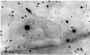
Figure 5: A 1995 Hale Telescope H$\alpha$ image of the Guitar Nebula (20 angstrom filter at 6564 angstroms). The cometary neck connecting to a spherical bubble are clearly evident. Credit: Chatterjee and Cordes (2002).

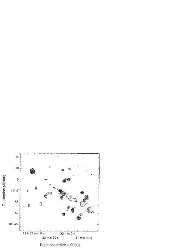
Figure 6: ROSAT X-ray surface brightness in the field of PSR1929+10 showing the X-ray tail. Wang et al. (1993) suggested that the X-ray morphology is due to the acceleration of particles behind the pulsar forming a relativistic backflow. North is up and East is left. Credit: Wang et al. (1993).

5.2 Identifying suitable input parameters

The outflow streams relativistically into the ambient medium generating a strong shock. We derive a value for the outflow pressure, $p_{o}$, from the assumption that the outflow is interacting with the ambient medium requiring that the momentum flux be comparable on either side of this shock; if the fluxes were not comparable, then either the ambient flow or outflow would dominate and the problem would be uninteresting. The momentum flux of the non-relativistic ambient medium and ultra-relativistic outflow are, respectively:

$$F_{M,a} = n_{a}v_{a}^{2}+p_{a}\rm,$$

$$F_{M,o} = \gamma_{o}^{2}(e_{o}+p_{o})v_{o}^{2}+p_{o}\rm.$$

For an ultra-relativistic outflow, $p_{o}\gg n_{o}\Rightarrow e_{o}\rightarrow 3p_{o}$, and $v_{o}\rightarrow 1$, and, for the ambient medium, $n_{a}v_{a}^{2}\gg p_{a}$. Applying these conditions, and noting that $\gamma_{o}^{2}p_{o}\gg p_{o}$, gives:

$$p_{o} \sim n_{a}\left(\frac{v_{a}}{2\gamma_{o}}\right)^{2}\sim 10^{-19}\;for\;\gamma_{o}\;=\;10^{6},\;n_{a}=1\rm.$$

We are then free to pick any $n_{o}$ meeting the conditions of a light, relativistic outflow, i.e. $n_{a},\;p_{o}\gg n_{o}$. This condition is motivated by the fact that the flow is very fast ($\gamma$ $>$ 10⁴). Well below the length scale of this study, the flow will be stabilized by the strong magnetic field, synchrotron cooling will be strong, and adiabatic losses due to expansion across the orders of magnitude in scale between the pulsar and the termination shock will sap internal energy. This will conspire to effectively stop energy from being converted into thermal motions. Under those conditions, the flow might be cold. However, on the scale of the termination shock the field is much weaker meaning far less synchrotron cooling, instability is less inhibited, and interesting evolution will occur over fewer adiabatic-loss scale lengths. Indeed, the flow might well be influenced by waves generated both upstream and downstream of the shock(s). The scales relevant to this work correspond to the region of “hot” post-termination shock plasma (e.g. Bucciantini, 2008) within a PWN. Therefore, a hot flow seems significantly more plausible than does a cold flow and we select $n_{o}=10^{-l}p_{o}$, $3<l<6$. This clearly satisfies $p_{o}\gg n_{o}$ and one may verify it satisfies $n_{a}\gg n_{o}$ by noting that the equation for $p_{o}$ implies $n_{a}\gg p_{o}$ since $\gamma_{o}^{2}\gg v_{a}^{2}$ for the flows of interest here.

5.3 A relativistic backflow

Fig. 7 shows a simulation of a $\gamma_{o}$ = 10⁵ outflow interacting with an ambient flow with velocity $v_{a}$ = 0.00583($\sim$1750 km s^-1). The outflow pressure was calculated for an ambient-flow velocity of 500 km s^-1 in order to match the typical value for pulsars in general. The outflow originates inside the circular region to the left of the evolving structure and the ambient flow streams in along the left edge of the computational domain. Fig. 8 shows the limited extent of the refined grid, supporting the choice of a maximum number of refinement level of L${}_{\mbox{max}}$ = 1. Recall the H$\alpha$ image of the Guitar Nebula (see Fig. 5), a well-known pulsar wind nebula with the most rapidly moving pulsar ever observed, with a transverse velocity of (1.7$\pm$0.4)$\times$10³ km s^-1 (Chatterjee and Cordes, 2002). The simulation qualitatively resembles the nebula. This result constitutes compelling motivation for the conclusion that interstellar-medium flows set up by the space motion of pulsars can indeed produce “cometary” nebulae.

Figure 7: An 871,200-iteration simulation of a light, ultra-relativistic outflow interacting with a dense, slow ambient flow. The input parameters are: $v_{a}$ = 0.00583 ($\sim$1750 km s^-1), $\mathcal{M}$ = 300, $n_{a}$ = 1, $\gamma_{o}$ = 10⁵, $p_{o}$= 7$\times$10^-16, and $n_{o}$ = 10${}^{-3}p_{o}$. The upper and lower panels show a linear color map of the rest-frame pressure and lab-frame mass density, respectively. Both have been reflected along the symmetry axis. The outflow originates within the circular region to the left of the evolving structure and the ambient flow streams in along the left edge of the domain. The lines labelled “1” and “2” are 1-D data cuts (hereafter “cut-h1”and “cut-h2”, respectively) with flow parameters plotted in Fig. 9.

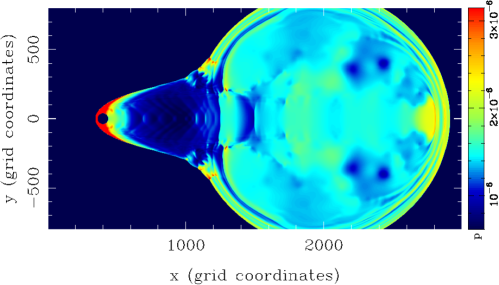
(a) Linear pressure map.

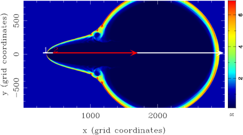
(b) Linear lab-frame mass density map.

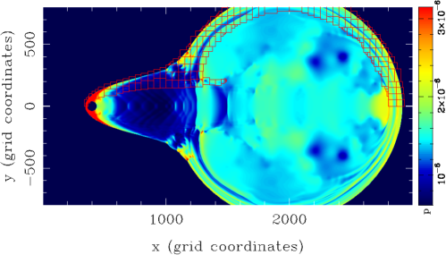
Figure 8: Plotted in red overlaying the pressure map for the simulation shown in Fig. 7 is the refined grid at level L=1. The bottom half of the map is a reflection of the top half and has the same refined grid even though it is not shown. Note that the red lines trace the outlines of the meshes of refined cells, but not the cells themselves. While the boundary shock is well-refined, the axial shocks within the nebula are not refined at all. Flagging is determined by the largest difference in R between adjacent cells for all cells at level L. The refinement only follows the boundary shock because R differences inside the nebula are small compared to the difference between the nebula and the ambient medium. We will investigate refinement flagging in more detail in a future study.

We believe this simulation to be the first demonstrating asymmetry arising from a spherically-symmetric, light, ultra-relativistic flow interacting with a dense, slow ambient flow. The lines labeled “1” and “2” on the density map in Fig. 7 mark one-dimensional cuts (hereafter “cut-h1”and “cut-h2”, respectively) made to probe the state of the simulation. Cut-h1 spans the entire structure while cut-h2 spans the interior space occupied by the pressure enhancements clearly visible in the pressure map. Fig. 9 shows the values of the flow parameters along these cuts. These plots clearly show the outer bounding shockwave represented by the red boundary in the density map as well as a series of weaker internal on-axis shocks visible in the pressure map. The x-component of the flow velocity shows that a relativistic back flow harboring a series of weak shocks has arisen down stream. This validates the interpretation by Wang et al. (1993) of the origin of the X-ray trail behind PSR1929+10, and demonstrates the ability of the refined solver to elucidate the internal structure of diffuse, ultra-relativistic pulsar wind nebulae which is often difficult to observe directly.

Figure 9: The run of the laboratory-frame mass (R), momentum (M), and total energy (E) densities, rest-frame mass (n), and total energy (e) densities, and pressure (p), Lorentz factor ($\gamma)$, x- and y-components of the flow velocity (v_x, v_y), the flow velocity (v), sound speed (c_s), and generalized Mach number ($\mathcal{M}$) along (a) cut-h1 and (b) cut-h2 in Fig. 7.

(a) Variables along cut-h1.

(b) Variables along cut-h2.

It is noteworthy that the termination shock of the wind is not evident in the simulation discussed above. This is due to numerical shocking of the wind as it emerges from the on-axis hemisphere, as follows. Consider the cells depicted in Fig. 10. Let the angle of the line connecting the center of the hemisphere and the center of a cell 1, 2, 3, or 4 be $\theta_{i}$, $i$ = 1, 2, 3, 4. Since we have taken the pulsar wind to be spherically symmetric as it emerges from the hemesphere, we may calculate the relative flow velocities $\Delta v_{12}$ and $\Delta v_{34}$ (normalized to the speed of light) at the centers of cells 1 & 2 and 3 & 4:

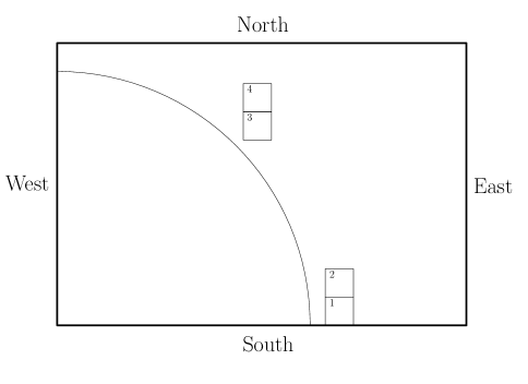
Figure 10: Schematic geometric cell layout pertaining to numerical shocking of the pulsar wind. The arc represents the on-axis hemisphere with radius 37.5 fine cells. Cell 1 is on-axis and is centered at 41.5 fine cells from the center of the hemisphere (relative center coordinates (x,y) = (41.5,0.5). The center coordinates of cells 2, 3, and 4 are (41.5,1.5), (29.5,29.5), and (29.5, 30.5) respectively.

$$\Delta v_{12} = \sqrt{\left(\frac{\cos\theta_{1}-\cos\theta_{2}}{1-\cos\theta_{1}\cos\theta_{2}}\right)^{2}+\left(\frac{\sin\theta_{1}-\sin\theta_{2}}{1-\sin\theta_{1}\sin\theta_{2}}\right)^{2}}$$

$$\approx 0.80\rm,$$

$$\Delta v_{34} = \sqrt{\left(\frac{\cos\theta_{3}-\cos\theta_{4}}{1-\cos\theta_{3}\cos\theta_{4}}\right)^{2}+\left(\frac{\sin\theta_{3}-\sin\theta_{4}}{1-\sin\theta_{3}\sin\theta_{4}}\right)^{2}}$$

$$\approx 0.03\rm.$$

This shows that the relative velocity between vertically adjacent on-axis cells just outside the hemisphere is supersonic relative to the pulsar outflow sound speed of 0.57 (for the parameters relevant to Fig. 7). Thus, the wind near the axis shocks immediately and is thermalized producing a post-termination shock flow. Given that at early times the wind shows no deviation from spherical symmetry (see Fig. 11), it is clear that this asymmetric numerical shocking of the wind is smeared out by the interaction with the ambient flow and does not impact the global evolution of the simulation.

Additional refinement levels, perhaps needed only at early simulation times, will mitigate the numerical shocking issue. However, since tests have shown such shocking is present with 3 levels, and the significant results discussed below were possible with 2 (i.e. L${}_{\mbox{max}}$ = 1), we leave explorations of additional refinement levels to future studies. When these studies result in unshocked, ultra-relativistic wind flows entering the computational domain, and the resolution of the termination shock, we will perform new shock-tube tests. However, while the refined REST_FRAME routine is essential for proper handling of the $\gamma>>1$ outflow, in the simulations presented here there are no structures involving Lorentz factors higher than those previously explored by Duncan and Hughes (1994) & Hughes et al. (2002) with the RHLLE solver for which shock-tube validation was performed. All structures referenced below originated in the computational domain where the the tried-and-true Newton-Raphson iterative solver was toggled into action (recall $\S$4). Therefore, we procede with firm confidence rooted in the previous shock-tube tests.

Figure 11: A time sequence of linear pressure maps for the simulation shown in Fig. 7. The sequence indicates that the appearance of the inflection point is preceded by a pressure drop inside the nebula. Note the finer time steps between 240K and 360K iterations and that the color map is relative to the minimum and maximum for each plot individually. However, the minimum is the same and the maximum is similar for all plots, so the variation is minimal.

(a) 10,000 iterations.

(b) 120,000 iterations.

(c) 240,000 iterations.

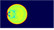
(d) 300,000 iterations.

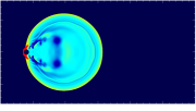
(e) 320,000 iterations.

(f) 360,000 iterations.

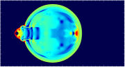
(g) 480,000 iterations.

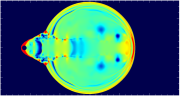
(h) 600,000 iterations.

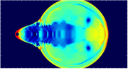
(i) 720,000 iterations.

6 Discussion

The physics behind the formation of the structure observed in Fig. 7 is as follows. The wind streams outward and sweeps up ambient material which drives pressure waves (weakly at first) into the shocked wind. As the nebula expands, the pressure inside decreases. Fig. 11 shows a series of pressure maps comprising a time development sequence for the simulation depicted in Fig. 7. The sequence clearly indicates that once the pulsar crosses the boundary of the initially spherical nebula, an inflection point develops along the leading edge at approximately 45^∘ from the axis as measured from W to N. The pressure waves are intensified and propagate to the axis and reflect, leading to the formation of a relativistic backflow harboring internal shockwaves reminiscent of shock diamonds. The fact that the backflow does not develop until after the inflection point supports this picture. The internal shockwaves, in turn, thermalize energy, allowing the flow to expand and inflate the trailing spherical bubble. As the bubble inflates, it “pinches” the inflection point enhancing the cuspy shape, maintaining the pressure-wave influx that sets up the energy-thermalizing backflow responsible for inflating the bubble. Such a feedback cycle is relevent to the Guitar nebula even though the pulsar was not born at the center of the trailing bubble – given its proper motion, the pulsar moves a distance corresponding to the entire nebula in less than 500 yr (Romani et al., 1997), a time orders of magnitude too short for the age of a pulsar powering a bow-shock nebula – because it explains how the bubble persists. Such a scenario is analogous to the formation of structure in relativistic galactic jets, where the evolution is driven by Kelvin-Helmholtz modes long the contact surface that separates the shocked ambient medium from the shocked jet material (e.g. Hughes et al., 2002).

The evolution of the Guitar-like shape is rather sensitive to the choice of parameters. As Tab. LABEL:tab:it-inf shows, the appearance of the inflection point marking the onset of the formation of the “neck” of the Guitar takes a significantly larger number of computational iterations as the ambient-flow velocity decreases. This is expected as the asymmetry of the nebula should evolve more slowly in this scenario: a decreased ambient-flow velocity is equivalent to a lower pulsar space motion and so it takes more time for the pulsar to reach the nebula boundary thereby delaying the formation of the inflection point. If the inflection point is not induced while the expanding nebula is small enough such that the ensuing neck is of significant scale, then no Guitar-like structure will be apparent. If a pulsar velocity of 1500 km s^-1, 1250 km s^-1, or 1000 km s^-1 is required for observable Guitar-like morphology to arise, then the velocity distribution of Arzoumanian et al. (2002) implies that $<$5%, 7-8%, or $\sim$15% of radio pulsars, respectively, have the possibility of developing such features depending on the nature of their ambient environment.

Table 3: The dependence of the Guitar-like inflection point on the number of simulation iterations. As expected, the higher the ambient-flow velocity, the sooner the inflection point develops due to the increased rate at which ambient material is swept-up.

Wind Lorentz factor	ambient-flow velocity	Iterations until inflection
(unitless)	(km s-1)	(104)
105
	1750	30
	1500	39
	1250	54
	1000	81
	750	unseen at 74
104
	5500	4
	4250	6
	3000	12
	1750	30

7 Conclusion

We discussed the application of an existing special relativistic, hydrodynamic (SRHD) primitive-variable recovery algorithm to ultra-relativistic flows (Lorentz factor, $\gamma$, of 10²–10⁶) and the refinement necessary for the numerical velocity root finder to work in this domain. We found that the velocity quartic, $Q(v)$, exhibits dual roots in the physical velocity range that move progressively closer together for larger $\gamma$ leading to a divide by zero and the failure of the Newton-Raphson iteration method employed by the existing primitives algorithm. Our solution was to recast the quartic to be a function, $Q(\gamma)$, of $\gamma$. We demonstrated that $Q(\gamma)$ exhibits only one physical root. However, Newton-Raphson iteration also failed in this case at high $\gamma$, due to the extreme slope of the quartic near the root, necessitating the use there of an analytical numerical root finder.

Our timing analysis indicated that using $Q(\gamma)$ with the 8-byte analytical root finder increased run time by only 24% compared to using $Q(v)$ with the 8-byte iterative root finder (based on 10 trial runs), while using $Q(\gamma)$ with the 16-byte analytical root finder ballooned run time by a factor of approximately 400. The iterative root finder is accurate to order 10^-4 for a sizable region of parameter space corresponding to Lorentz factors on the order of 10² and smaller. Therefore, we implemented a computational switch that checks the values of $M/E$ and $R/E$ and calls the iterative or analytical root finder accordingly thereby creating a hybrid primitives recovery algorithm called REST_FRAME.

In addition, our exploration of parameter space suggests that the discriminant of the cubic resolvent (as defined by Eqn. 9 in $\S$3.1) will always be positive for physical flows. Therefore, we did not include code for negative discriminants in our routine. Formal proof remains elusive, however, leaving potential for future work.

We have shown that REST_FRAME is capable of calculating the primitive variables from the conserved variables to an accuracy of at least $O(10^{-4})$ for Lorentz factors up to 10⁶ with significantly better accuracy for Lorentz factors $\leq 10^{5}$, and slightly worse (order 10^-3) for a small portion of the space corresponding to the highest Lorentz factors. We traced the degradation in accuracy for larger Lorentz factors to the effect of subtractive cancellation. Past studies have shown that an accuracy of order 10^-4 is capable of robustly capturing hydrodynamic structures. We have applied the refined solver to an ultra-relativistic problem and have shown that it is capable of reproducing observed structures and is well-suited to our study of the internal structure of diffuse pulsar wind nebulae.

Our main conclusions are as follows:

• Relativistic, hydrodynamic simulations have shown that the relatively slow, dense ISM flow resulting from the space motion of a pulsar can set up an interaction with the extremely light, ultra-relativistic pulsar wind leading to an asymmetric nebula with a morphology reminiscent of the Guitar nebula.

• Simulations have validated the interpretation that a relativistic backflow behind PSR1929+10 is responsible for the X-ray morphology. Results further show that the backflow can harbor a series of internal shockwaves that inflates a nebular bubble, and that the bubble provides positive feedback to the backflow, explaining how the Guitar bubble persists.

• The evolution of the bubble/backflow structure is sensitive to the choice of input parameters justifying a future series of simulation runs that will determine what pulsar velocities and wind/ISM density ratios are required for the bubble/backflow feedback loop to arise.

References

- Arzoumanian et al. (2002) Arzoumanian, Z., Chernoff, D. F., Cordes, J. M., Mar. 2002. The Velocity Distribution of Isolated Radio Pulsars. ApJ, 568, 289–301.
- Bronshtein and Semendyayev (1997) Bronshtein, I. N., Semendyayev, K. A., 1997. Handbook of Mathematics, ed. K. A. Hirsch, 3rd Edition. Springer-Verlag Telos.
- Bucciantini (2008) Bucciantini, N., 2008. Modeling Pulsar Wind Nebulae. Advances in Space Research 41, 491–502.
- Bucciantini et al. (2005) Bucciantini, N., Amato, E., Del Zanna, L., Apr. 2005. Relativistic MHD simulations of pulsar bow-shock nebulae. A&A, 434, 189–199.
- Chatterjee and Cordes (2002) Chatterjee, S., Cordes, J. M., Aug. 2002. Bow Shocks from Neutron Stars: Scaling Laws and Hubble Space Telescope Observations of the Guitar Nebula. ApJ, 575, 407–418.
- Cordes and Chernoff (1998) Cordes, J. M., Chernoff, D. F., Sep. 1998. Neutron Star Population Dynamics. II. Three-dimensional Space Velocities of Young Pulsars. ApJ, 505, 315–338.
- Cordes et al. (1993) Cordes, J. M., Romani, R. W., Lundgren, S. C., Mar. 1993. The Guitar nebula - A bow shock from a slow-spin, high-velocity neutron star. Nature, 362, 133–135.
- Del Zanna et al. (2004) Del Zanna, L., Amato, E., Bucciantini, N., Jul. 2004. Axially symmetric relativistic MHD simulations of Pulsar Wind Nebulae in Supernova Remnants. On the origin of torus and jet-like features. A&A, 421, 1063–1073.
- Del Zanna and Bucciantini (2002) Del Zanna, L., Bucciantini, N., Aug. 2002. An efficient shock-capturing central-type scheme for multidimensional relativistic flows. I. Hydrodynamics. A&A, 390, 1177–1186.
- Del Zanna et al. (2003) Del Zanna, L., Bucciantini, N., Londrillo, P., Mar. 2003. An efficient shock-capturing central-type scheme for multidimensional relativistic flows. II. Magnetohydrodynamics. A&A, 400, 397–413.
- Delettrez et al. (2005) Delettrez, J. A., Myatt, J., Radha, P. B., Stoeckl, C., Skupsky, S., Meyerhofer, D. D., Dec. 2005. Hydrodynamic simulations of integrated experiments planned for the OMEGA/OMEGA EP laser systems. Plasma Physics and Controlled Fusion 47, B791–B798.
- Duncan and Hughes (1994) Duncan, G. C., Hughes, P. A., Dec. 1994. Simulations of relativistic extragalactic jets. ApJ, 436, L119–L122.
- Emmering and Chevalier (1987) Emmering, R. T., Chevalier, R. A., Oct. 1987. Shocked relativistic magnetohydrodynamic flows with application to pulsar winds. ApJ, 321, 334–348.
- Fryxell et al. (2000) Fryxell, B., Olson, K., Ricker, P., Timmes, F. X., Zingale, M., Lamb, D. Q., MacNeice, P., Rosner, R., Truran, J. W., Tufo, H., Nov. 2000. FLASH: An Adaptive Mesh Hydrodynamics Code for Modeling Astrophysical Thermonuclear Flashes. ApJS, 131, 273–334.
- Gaensler and Slane (2006) Gaensler, B. M., Slane, P. O., Sep. 2006. The Evolution and Structure of Pulsar Wind Nebulae. ARA&A, 44, 17–47.
- Gammie et al. (2003) Gammie, C. F., McKinney, J. C., Tóth, G., May 2003. HARM: A Numerical Scheme for General Relativistic Magnetohydrodynamics. ApJ, 589, 444–457.
- Godunov (1959) Godunov, S. K., 1959. Difference Methods for the Numerical Calculations of Discontinuous Solutions of the Equations of Fluid Dynamics. Mat. Sb. 47, 271–306, in Russian, translation in: US Joint Publ. Res. Service, JPRS, 7226 (1969).
- Heger et al. (2003) Heger, A., Fryer, C. L., Woosley, S. E., Langer, N., Hartmann, D. H., Jul. 2003. How Massive Single Stars End Their Life. ApJ, 591, 288–300.
- Hirano (2004) Hirano, T., Aug. 2004. Hydrodynamic models. Journal of Physics G Nuclear Physics 30, S845–S851.
- Hughes (2005) Hughes, P. A., Mar. 2005. The Origin of Complex Behavior of Linearly Polarized Components in Parsec-Scale Jets. ApJ, 621, 635–642.
- Hughes et al. (2002) Hughes, P. A., Miller, M. A., Duncan, G. C., Jun. 2002. Three-dimensional Hydrodynamic Simulations of Relativistic Extragalactic Jets. ApJ, 572, 713–728.
- Ibanez (2003) Ibanez, J. M., 2003. Numerical Relativistic Hydrodynamics. In: Fernández-Jambrina, L., González-Romero, L. M. (Eds.), Current Trends in Relativistic Astrophysics. Vol. 617 of Lecture Notes in Physics, Berlin Springer Verlag. pp. 113–129.
- Kargaltsev and Pavlov (2008) Kargaltsev, O., Pavlov, G. G., Jan. 2008. Pulsar Wind Nebulae in the Chandra Era. ArXiv e-prints 801. Available from: http://adsabs.harvard.edu/ abs/2008AIPC..983..171K.
- Kennel and Coroniti (1984a) Kennel, C. F., Coroniti, F. V., Aug. 1984a. Confinement of the Crab pulsar’s wind by its supernova remnant. ApJ, 283, 694–709.
- Kennel and Coroniti (1984b) Kennel, C. F., Coroniti, F. V., Aug. 1984b. Magnetohydrodynamic model of Crab nebula radiation. ApJ, 283, 710–730.
- Komissarov (1999) Komissarov, S. S., Feb. 1999. A Godunov-type scheme for relativistic magnetohydrodynamics. MNRAS, 303, 343–366.
- Martí and Müller (2003) Martí, J. M., Müller, E., Dec. 2003. Numerical Hydrodynamics in Special Relativity. Living Reviews in Relativity 6.
- Michel (1969) Michel, F. C., Nov. 1969. Relativistic Stellar-Wind Torques. ApJ, 158, 727–738.
- Michel (1973) Michel, F. C., Mar. 1973. Rotating Magnetospheres: an Exact 3-D Solution. ApJ, 180, L133–L137.
- Mignone and McKinney (2007) Mignone, A., McKinney, J. C., Jul. 2007. Equation of state in relativistic magnetohydrodynamics: variable versus constant adiabatic index. MNRAS, 378, 1118–1130.
- Noble (2003) Noble, S. C., Oct. 2003. A Numerical Study of Relativistic Fluid Collapse. ArXiv General Relativity and Quantum Cosmology e-prints.
- Noble et al. (2006) Noble, S. C., Gammie, C. F., McKinney, J. C., Del Zanna, L., Apr. 2006. Primitive Variable Solvers for Conservative General Relativistic Magnetohydrodynamics. ApJ, 641, 626–637.