Smooth Light Curves from a Bumpy Ride: Relativistic Blast Wave Encounters a Density Jump

Abstract

Some gamma-ray burst (GRB) afterglow light curves show significant variability, which often includes episodes of rebrightening. Such temporal variability had been attributed in several cases to large fluctuations in the external density, or density ”bumps”. Here we carefully examine the effect of a sharp increase in the external density on the afterglow light curve by considering, for the first time, a full treatment of both the hydrodynamic evolution and the radiation in this scenario. To this end we develop a semi-analytic model for the light curve and carry out several elaborate numerical simulations using a one dimensional hydrodynamic code together with a synchrotron radiation code. Two spherically symmetric cases are explored in detail – a density jump in a uniform external medium, and a wind termination shock. The effect of density clumps is also constrained. Contrary to previous works, we find that even a very sharp (modeled as a step function) and large (by a factor of $a\gg 1$) increase in the external density does not produce sharp features in the light curve, and cannot account for significant temporal variability in GRB afterglows. For a wind termination shock, the light curve smoothly transitions between the asymptotic power laws over about one decade in time, and there is no rebrightening in the optical or X-rays that could serve as a clear observational signature. For a sharp jump in a uniform density profile we find that the maximal deviation $\Delta\alpha_{\rm max}$ of the temporal decay index $\alpha$ from its asymptotic value (at early and late times), is bounded (e.g, $\Delta\alpha_{\rm max}<0.4$ for $a=10$); $\Delta\alpha_{\rm max}$ slowly increases with $a$, converging to $\Delta\alpha_{\rm max}\approx 1$ at very large $a$ values. Therefore, no optical rebrightening is expected in this case as well. In the X-rays, while the asymptotic flux is unaffected by the density jump, the fluctuations in $\alpha$ are found to be comparable to those in the optical. Finally, we discuss the implications of our results for the origin of the observed fluctuations in several GRB afterglows.

1 Introduction

Gamma-ray bursts (GRBs) are produced by a relativistic outflow from a compact source. The outflow sweeps up the external medium and drives a strong relativistic shock into it. Eventually the outflow is decelerated (by $pdV$ work across the contact discontinuity that separates the ejecta and the shocked external medium) and most of the kinetic energy is transferred to the shocked external medium (for recent reviews see Piran 2005; Meszaros 2006). The shocked external medium produces long lived afterglow emission that is detected in the X-rays, optical, and radio for days, weeks, and months, respectively, after the GRB. The afterglow emission is thought to be predominantly synchrotron radiation. This is supported both by the broad band spectrum and by the detection of linear polarization at the level of a few percent in the optical (or near infrared) afterglow of several GRBs (see Covino, 2003, and references therein). Inverse-Compton scattering of the synchrotron photons might dominate the observed flux in the X-rays in some cases (Panaitescu & Kumar, 2000; Sari & Esin, 2001; Harrison et al., 2001).

In the pre-Swift era the best monitoring of GRB afterglow light curves was, by far, in the optical. Most afterglow light curves showed a smooth power law decay (Stanek et al., 1999; Laursen, & Stanek, 2003; Gorosabel et al., 2006), and often also a smooth achromatic transition to a steeper power law decay that is attributed to the outflow being collimated into a narrow jet (Rhoads, 1999; Sari, Piran & Halpern, 1999). It has been argued (Wang & Loeb, 2000) that the smoothness of the afterglow light curve is directly related to (and thus enables to constrain) the smoothness of the external density field. Nevertheless, some optical afterglows have shown significant temporal variability, with strong deviations from the more typical smooth power law behavior. The best examples are GRBs 021004 (Pandey et al., 2002; Fox et al., 2003; Bersier et al., 2003) and 030329 (Matheson et al., 2003; Sato et al., 2003; Uemura et al., 2004; Lipkin et al., 2004).

Possible explanations for such temporal variability in GRB afterglow light curves include variations in the external density (Wang & Loeb, 2000; Lazzati et al., 2002; Nakar, Piran & Granot, 2003), or in the energy of the afterglow shock. The latter includes energy injection by “refreshed shocks” – slower shells of ejecta that catch up with the afterglow shock on long time scales (Rees & Mészáros, 1998; Kumar & Piran, 2000a; Sari & Mészáros, 2000; Ramirez-Ruiz, Merloni & Rees, 2001; Granot, Nakar & Piran, 2003) or a “patchy shell” – angular inhomogeneities within the outflow (Kumar & Piran, 2000b; Nakar, Piran & Granot, 2003; Heyl & Perna, 2003; Nakar & Oren, 2004). Another possible cause for variability in the afterglow light curve, although it is expected to be quite rare, is microlensing by an intervening star in a galaxy that happens to be close to our line of sight. GRB 000301C exhibited an achromatic bump in its optical to NIR light curves that peaked after $\sim 4\;$days (Sagar et al., 2000; Berger et al., 2000) which had been interpreted as such a microlensing event (Garnavich, Loeb & Stanek, 2000; Gaudi, Granot & Loeb, 2001; Baltz & Hui, 2005), although other interpretations such as a bump in the external density have also been suggested (Berger et al., 2000).

Recent observations by Swift have found flares in the early X-ray afterglows of many GRBs (Burrows et al., 2005; Nousek et al., 2006; Falcone et al., 2006; O’brien et al., 2006) which are probably due to late time activity of the central source (Nousek et al., 2006; Zhang et al., 2006). Early optical variability also appears to be more common than previously thought (e.g., Stanek et al., 2006), although it is not yet clear if it is caused by similar mechanisms as the late time optical variability that had been detected before Swift.

The most natural forms of variations in the external density are either clumps on top of a smooth background density distribution, or a global abrupt change in density with radius. The latter can be, e.g., the termination shock of the wind from the massive star progenitor of a long-soft GRB (Wijers, 2001). Such a stellar wind environment may have a richer structure and can include an abrupt increase in density with radius at the contact discontinuity between shocked wind from two different evolutionary stages of the progenitor star, as well as clumps that are formed due to Rayleigh-Taylor instability (Ramirez-Ruiz et al., 2005; Eldridge et al., 2006). Density clumps with a mild density contrast may also be formed due to turbulence in the external medium. Furthermore, the external density profile is expected to vary between different progenitor models (Fryer, Rockefeller & Young, 2006). The variability that had been observed in optical afterglows was attributed to density clumps in the external medium (Lazzati et al., 2002; Nakar, Piran & Granot, 2003). The expected observational signatures of the afterglow shock running into the wind termination shock of the massive star progenitor have also been considered (Wijers, 2001; Ramirez-Ruiz et al., 2001, 2005; Eldridge et al., 2006; Pe’er & Wijers, 2006). In all these cases it has been argued that there would be a clear observational signature in the form of a rebrightening in the afterglow light curve, before approaching the new shallower decay slope corresponding to the uniform density of the shocked wind.

Here we revisit the effect of density fluctuations on the afterglow light curve by solving in detail the case of a spherically symmetric external density with a single density jump (by a factor of $a>1$) at some radius $R_{0}$, while the density at smaller and larger radii is a (generally different) power law in radius. This is done by constructing a semi-analytic model for the observed flux due to synchrotron emission at different power law segments of the spectrum and by carrying out numerical simulations. The semi-analytic model takes into account the effect of the reverse shock on the hydrodynamics and on the emissivity, as well as the effect of the spherical geometry on the arrival time of photons to the observer. Being semi-analytic, however, this model uses some approximations for the hydrodynamic evolution and the resulting radiation. Therefore, we also perform numerical simulations in which the light curves are calculated using a hydrodynamic+radiation numerical code. This code self-consistently calculates the radiation and evolves the electron distribution in every fluid element, which corresponds to a computational cell of the one dimensional Lagrangian hydrodynamic code. The results of this code are used to obtain light curves in cases of special interest and near spectral break frequencies, as well as to verify the quality of the semi-analytic model, which is found to agree well with the numerical results. These calculations are much more accurate than those presented in previous works, and our results are significantly different. In all cases we find a very smooth transition to the new asymptotic power law, with no rebrightening for an initially decaying light curve.

In §2 we develop the semi-analytic model. First, in §2.1 a simple analytic model is constructed for the hydrodynamics, which agrees very well with our numerical results. Then, in §2.2 we construct a semi-analytic model for the observed flux density. Specific case studies (§3) are then analyzed in detail, for a wind termination shock (§3.1) and for a spherical density jump in a uniform medium (§3.2). The light curves for these cases are also calculated using the numerical code (described in Appendix A). The effect of proximity to a break frequency around the time of the density jump is investigated in §3.3, and our main conclusions are found to remain valid also in the vicinity of the break frequencies. §4 is devoted to a discussion of the expected observational signatures of density clumps on top of a smooth underlying external density distribution. Such density clumps are found to have a very weak observational signature which would be very hard to detect. In §5 we discuss the implications of our results for the origin of the observed fluctuations in several GRB afterglows. Our conclusions are discussed in §6.

2 Semi-Analytic model for a Spherical Jump in the External Density

In this section we model a spherical relativistic blast wave that propagates into a power-law external density profile ($\rho_{\rm ext}=Ar^{-k}$ with $k<3$) which has a single sharp density jump (by a factor $a>1$) at some radius $r=R_{0}$. The power law index, $k$, of the external density is allowed to be different at $r<R_{0}$ ($k_{0}$) and at $r>R_{0}$ ($k_{1}$).

The hydrodynamic evolution, as well as the resulting contribution to the light curves, can be roughly separated into three phases corresponding to the following ranges of the radius $R$ of the forward shock: (i) at $R<R_{0}$ the blast-wave follows a self-similar evolution (Blandford & McKee, 1976, BM hereafter), (ii) at $R=R_{0}$ a reverse shock forms which crosses most of the shell of previously shocked material (that had been swept up at $r<R_{0}$) at $R=R_{1}$, while the forward shock continues ahead of the density jump but with a reduced Lorentz factor, (iii) at $R>R_{1}$ the forward shock relaxes into a new self-similar evolution corresponding to the new density profile at $r>R_{0}$. In the following we first approximate the hydrodynamic evolution of the different shocks during these three phases and then calculate the resulting light curves.

2.1 Hydrodynamics

Consider a spherical ultra-relativistic blast wave (identified with the afterglow shock), which is well described by the self-similar BM solution at $R<R_{0}$, that propagates into the following external density profile:

$$\rho_{\rm ext}=\left\{\begin{matrix}A_{0}r^{-k_{0}}&\ \ r<R_{0}\ ,\cr\cr A_{1}r^{-k_{1}}&\ \ r>R_{0}\ .\end{matrix}\right.$$ (1)

The amplitude of the density jump, i.e. the factor by which the density increases at $r=R_{0}$, is given by

$$a\equiv\lim_{\epsilon\to 0}\frac{\rho_{\rm ext}[(1+\epsilon)R_{0}]}{\rho_{\rm ext}[(1-\epsilon)R_{0}]}=\frac{A_{1}}{A_{0}}R_{0}^{k_{0}-k_{1}}\ ,$$ (2)

and is assumed to be larger than unity. The afterglow shock encounters the jump in the external density profile at a lab frame time $t_{0}=[1+1/2(4-k_{0})\Gamma_{4}^{2}]R_{0}/c\approx R_{0}/c$, where $c$ is the speed of light ,$\Gamma_{4}$ is the Lorentz factor of the shock front just before it encounters the density bump at $r=R_{0}$, and the corresponding Lorentz factor of the fluid just behind the shock is denoted by $\gamma_{4}=\Gamma_{4}/\sqrt{2}$. At $t<t_{0}$ there are three regions: the region behind the afterglow shock (subscript ‘4’) is described by the BM solution with $(A,k)=(A_{0},k_{0})$, and the two regions of cold unperturbed external medium (subscripts ‘0’ and ‘1’ at $r<R_{0}$ and $r>R_{0}$, respectively).

When the afterglow shock encounters the jump in the external density a reverse shock is driven into the hot BM shell, while a forward shock propagates into the cold higher density external medium at $r>R_{0}$. At this stage region ‘0’ no longer exists, but two new regions are formed so that altogether there are four regions: (i) the cold unperturbed external medium ahead of the forward shock with a density $\rho_{\rm ext}=A_{1}r^{-k_{1}}$, (ii) the shocked external medium originating from $r>R_{0}$, (iii) the portion of the BM shell that has been shocked by the reverse shock (corresponding to doubly shocked external medium originating at $r<R_{0}$), and (iv) the unperturbed portion of the BM solution which has not yet been shocked by the reverse shock (i.e. singly shocked external medium originating from $r<R_{0}$). These regions are denoted by subscripts ‘1’ through ‘4’, respectively. Regions 2 and 3 are separated by a contact discontinuity.

Immediately after $t_{0}$ [or more precisely, at $0<(t-t_{0})/t_{0}\ll a^{-1/2}$] the reverse shock reaches only a very small part of the BM profile (just behind the contact discontinuity) which corresponds to values $\chi-1\ll 1$ of the self similar variable, $\chi$ (defined in Blandford & McKee, 1976), so that at this early stage the conditions in this region may be approximated as being constant with the values just behind the shock for the BM profile with $(A,k)=(A_{0},k_{0})$ at $t=t_{0}$ (i.e. when the shock radius is $R=R_{0}$). Since we are interested in a small range in radius, $\Delta R\ll R_{0}$, we can use a planar geometry and solve the relevant Riemann problem. Region 4 is described by the BM solution while in region 1 we have $\rho_{1}=w_{1}/c^{2}=n_{1}m_{p}=A_{1}r^{-k_{1}}$, $p_{1}=e_{1}=0$ and $\gamma_{1}=1$, where $m_{p}$ is the proton mass. The pressure $p$, internal energy density $e$, enthalpy density $w$, rest mass density $\rho$, and number density $n$ are measured in the proper frame (i.e. the fluid rest frame). We consider a relativistic afterglow shock, $\gamma_{4}\gg 1$, and a density contrast which is not too large such that even after the afterglow shock crosses the density bump it will still be relativistic (i.e. $\gamma_{4}\gg\psi\sim a^{1/4}$, see equation [3]). Under these conditions, in regions 2 and 3 the fluid is relativistically hot, $\rho_{2}c^{2}\ll p_{2}$ and $\rho_{3}c^{2}\ll p_{3}$. Therefore, the adiabatic index in regions 2, 3 and 4 is $4/3$, implying $p_{i}=e_{i}/3=w_{i}/4$ in these regions. This leaves eight unknown quantities: $\gamma$, $n$ and $e$ in regions 2 and 3, as well as the Lorentz factors of the reverse shock, $\Gamma_{r}$, and of the forward shock, $\Gamma_{f}$. Correspondingly, there are eight constraints: three from the shock jump conditions at each of the two shocks, and two at the contact discontinuity: $e_{2}=e_{3}$ and $\gamma_{2}=\gamma_{3}$. The shock jump conditions simply state the conservation of energy, momentum, and particle number across the shock, which is equivalent to the continuity of their corresponding fluxes. At the rest frame of the shock front they correspond to the continuity of $w\gamma^{2}v$, $w\gamma^{2}(v/c)^{2}+p$, and $n\gamma v$, respectively, across the shock (where $v$ is the fluid velocity measured in that frame, while $p$, $n$, and $w$ are measured in the rest frame of the fluid). Unless stated otherwise, all velocities and Lorentz factors are measured in the rest frame of the unperturbed external medium, which is identified with the lab frame where the flow is spherical.

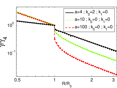
Figure 1: The Lorentz factor of the forward shock as function of radius for three different density profiles that are described by Eq. (1)  (see legend for the parameters of each profile). The solid lines show our analytic approximation (Eq. [6]) while the dots are the results of a hydrodynamic simulation.

Under the above assumptions and for $\gamma_{2}=\gamma_{3}\gg 1$ we obtain

$$\left(\frac{\gamma_{4}}{\gamma_{3}}\right)^{2}\equiv\psi^{2}=\frac{3a-4}{\sqrt{\frac{12}{a}}(a-1)\,-1}\ ,$$ (3)

In the limit of a relativistic reverse shock ($a\gg 1$) Eq. (3) reduces to $\psi=\gamma_{4}/\gamma_{3}\approx(3a/4)^{1/4}$.

The Lorentz factor, $\gamma$, of the fluid behind the forward shock as a function of  $\tilde{R}\equiv R/R_{0}$ is $\gamma(\tilde{R}<1)=\gamma_{4}\tilde{R}^{(3-k_{0})/2}$ before the density jump and $\gamma=\psi^{-1}\gamma_{4}$ immediately after the density jump. A simple and useful analytic model for $\gamma(\tilde{R}>1)$ is obtained using the energy conservation equation while replacing the mass collected up to $R_{0}$, $M_{0}=4\pi A_{0}R_{0}^{3-k_{0}}/(3-k_{0})$, by an effective mass $M_{{\rm eff},0}=\psi^{2}M_{0}$. The reasoning behind the factor of $\psi^{2}$ is to account for the fact that just after the density jump the bulk Lorentz factor and the average particle random Lorentz factor in region 4 ($\gamma_{4}$) is a factor of $\psi$ higher than that in region 2 ($\gamma_{2}=\gamma_{3}$), so that the energy in region 4 is $\approx M_{0}\gamma_{4}^{2}=\psi^{2}M_{0}\gamma^{2}$. As a result the expression for energy conservation at $R>R_{0}$ is approximated by

$$E=\left[C_{0}\psi^{2}M_{0}+C_{1}M_{1}(R)\right]\gamma^{2}(R)c^{2}={\rm const}\ ,$$ (4)

where $C_{i}=4(3-k_{i})/(17-4k_{i})$ (this is valid for $k_{i}<3$), and

$$M_{1}=\int_{R_{0}}^{R}4\pi r^{2}dr\rho_{\rm ext}(r)=M_{0}\left(\frac{3-k_{0}}{3-k_{1}}\right)a\left(\tilde{R}^{3-k_{1}}-1\right)\ .$$ (5)

According to our simple model,

$$\gamma(\tilde{R}>1)=\gamma_{4}\left[\psi^{2}+\left(\frac{17-4k_{0}}{17-4k_{1}}\right)a\left(\tilde{R}^{3-k_{1}}-1\right)\right]^{-1/2}\ .$$ (6)

Figure 1 shows a comparison of our simple analytic expression with the results of a hydrodynamic simulation (see appendix A for the simulation details). It depicts the forward shock Lorentz factor as a function of radius for a spherical ultra-relativistic blast-wave that propagates into three different density profiles of the external medium that are described by equation (1). Two of the density profiles are uniform both below and above $R_{0}$ ($k_{0}=k_{1}=0$) with density jumps of $a=10$ and $a=100$ at $R_{0}$. The third density profile presents a wind termination shock, for which $k_{0}=2$, $k_{1}=0$, and $a=4$. Figure 1 demonstrates that despite the simplicity of our analytic approximation, it provides an excellent description of the accurate solution.

Once the reverse shock reaches $\chi\gtrsim 2$, it samples most of the energy in the BM radial profile. At this stage a good fraction of the total energy is already in region 2, and a similar energy is in region 3. A rough estimate for the radius, $R_{1}=R_{0}+\Delta R$, at which this occurs may be obtained by using the conditions in region 2 that have been calculated above according to the shock jump conditions for a uniform shell, and checking when most of the energy will be in region 2. This occurs after a mass $\approx\psi^{2}M_{0}$ is swept from $r>R_{0}$, i.e. when the two terms in Eq. 6 become comparable, which corresponds to $(\tilde{R}^{3-k_{1}}-1)=a^{-1}\psi^{2}[(17-4k_{1})/(17-4k_{0})]\sim a^{-1/2}$, or

$$\tilde{R}_{1}=\left[1+\frac{\psi^{2}}{a}\left(\frac{17-4k_{1}}{17-4k_{0}}\right)\right]^{1/(3-k_{1})}\ .$$ (7)

For $a\gg 1$ this simplifies to $\Delta R/R_{0}\approx a^{-1/2}\sqrt{3}(17-4k_{1})/[2(17-4k_{0})(3-k_{1})]\sim a^{-1/2}\ll 1$. Once $E/\gamma^{2}c^{2}=C_{0}\psi^{2}M_{0}+C_{1}M_{1}=M_{\rm eff}$ becomes comparable to the mass that would have been swept up at the same radius if the outer density profile was valid everywhere, $4\pi A_{1}R^{3-k_{1}}/(3-k_{1})$, the dynamics approach the new BM self similar solution for $(A,k)=(A_{1},k_{1})$. By this time $M_{\rm eff}(R)$ is dominated by the second term in Eq. 4, and therefore the new BM solution is approached when $\tilde{R}^{3-k_{1}}-1$ becomes comparable to $\tilde{R}^{3-k_{1}}$, i.e. when $\tilde{R}\gtrsim\tilde{R}_{\rm BM}=2^{1/(3-k_{1})}$.

2.2 The Resulting Light Curve

Here the simplified description of the hydrodynamics presented above is used in order to obtain a semi-analytic expression for the resulting light curve. We obtain explicit expressions for the three most relevant power-law segments (PLSs) of the synchrotron spectrum: $\nu<\nu_{m}<\nu_{c}$, $\nu_{m}<\nu<\nu_{c}$, and $\nu>\max(\nu_{m},\nu_{c})$, where $\nu_{m}$ is the typical synchrotron frequency and $\nu_{c}$ is the cooling frequency. The first two PLSs appear in the slow cooling regime ($\nu_{m}<\nu_{c}$) while the last PLS also appears in the fast cooling regime ($\nu_{m}>\nu_{c}$).

Two useful time scales for calculating the observed radiation are the radial time, $T_{r}(R)=t-R/c$, and the angular time, $T_{\theta}(R)=R/2c\gamma^{2}$. The radial time is the arrival time of a photon emitted at the shock front at radius $R$ along the line of sight (at $\theta=0$) relative to a photon emitted at $t=0$ at $R=0$. The angular time is the arrival time of a photon emitted at the shock front at an angle of $\theta=\gamma^{-1}$ from the line of sight relative to a photon emitted at the shock front at the same radius $R$ along the line of sight. For convenience we normalize the observed time by $T_{0}=T_{r}(R_{0})=R_{0}/4(4-k_{0})c\gamma_{4}^{2}$, $\tilde{T}\equiv T/T_{0}$. In our simple model the radial and angular times are given by

$$\tilde{T}_{r}(\tilde{R}>1) = 1+\left[\psi^{2}-\left(\frac{17-4k_{0}}{17-4k_{1}}\right)a\right](4-k_{0})\left(\tilde{R}-1\right)$$ (8)

$$+\left(\frac{4-k_{0}}{4-k_{1}}\right)\left(\frac{17-4k_{0}}{17-4k_{1}}\right)a\left(\tilde{R}^{4-k_{1}}-1\right)\ ,$$

$$\tilde{T}_{\theta}(\tilde{R}>1) = 2(4-k_{0})\tilde{R}\left[\psi^{2}+\left(\frac{17-4k_{0}}{17-4k_{1}}\right)a\left(\tilde{R}^{3-k_{1}}-1\right)\right]\ ,\quad$$ (9)

while

$$\tilde{T}_{r}(\tilde{R}<1)=\tilde{R}^{4-k_{0}}\ ,\quad\tilde{T}_{\theta}(\tilde{R}<1)=2(4-k_{0})\tilde{R}^{4-k_{0}}\ .$$ (10)

Following Nakar & Piran (2003), we express the observed flux as an integral over the radius $R$ of the forward shock. It is convenient to express the integrand, which represents the contribution from a given radius $R$ to the observed flux at a given observed time $T$, as the product of two terms: the total emissivity (per unit frequency) of the blast-wave between $R$ and $R+dR$, $A_{\nu}(R)$, and a weight function, $g(\tau,\beta)$, where $\beta=d\log F_{\nu}/d\log\nu$ is the spectral slope, which takes into account the relative contribution from a given radius $R$ to the observed flux at a given observed time $T$:

$$\tilde{F}_{\nu}(\tilde{T})=C(\beta)\int_{0}^{\tilde{R}_{max}(\tilde{T)}}d\tilde{R}\,\,\tilde{A}_{\nu}\,g(\tau,\beta)\ .$$ (11)

For convenience all variables are normalized by their value at $T_{0}$ or $R_{0}$: $\tilde{F}_{\nu}(\tilde{T})\equiv F_{\nu}(T=\tilde{T}T_{0})/F_{\nu}(T_{0})$ and $\tilde{A}_{\nu}(\tilde{R})\equiv A_{\nu}(R=\tilde{R}R_{0})/A_{\nu}(R_{0})$. The normalization constant $C(\beta)$ may be obtained by the requirement that $\tilde{F}_{\nu}(\tilde{T}=1)=1$, while $\tilde{R}_{\rm max}(\tilde{T})$ is given by $T_{r}[\tilde{R}_{\rm max}(\tilde{T})]=\tilde{T}$ and may be obtained by inverting equation 8 for $\tilde{R}$. The weight function $g(\tau,\beta)$ depends on the the dimensionless “time” variable

$$\tau(\tilde{R},\tilde{T})\equiv\frac{\tilde{T}-\tilde{T}_{r}(\tilde{R})}{\tilde{T}_{\theta}(\tilde{R})}\ ,$$ (12)

and on the PLS where the observed frequency $\nu$ is in, which is specified by the value of the spectral index $\beta$ ($F_{\nu}\propto\nu^{\beta}$). In principle, during the self-similar phase, for $\nu<\nu_{c}$, $g$ has a complicated form and it also depends on the power law index, $k$, of the external density (Nakar & Piran, 2003). However, the whole approach that is adopted here (of separating the integrand into the product of $A_{\nu}$ and a relatively simple $g$ where the time dependence is only through $\tau$) is anyway not strictly valid during the non-self-similar phase. Therefore, we choose to use the simplest expression of $g$ at all PLSs, which is the expression obtained in the thin emitting region approximation (which is accurate for $\nu>\nu_{c}$),

$$g(\tau,\beta)=(1+\tau)^{\beta-2}\ .$$ (13)

An approximation for $\tilde{A}_{\nu}(\tilde{R})$ is obtained by considering three different phases of emission: $\tilde{R}<1$, $1<\tilde{R}<\tilde{R}_{1}$, and $\tilde{R}>\tilde{R}_{1}$ (similar to the approach taken by Pe’er & Wijers 2006). For $\tilde{R}<1$ the blast-wave is self-similar and $\tilde{A}_{\nu}(\tilde{R}<1)$ is similar to the one calculated in Nakar & Piran (2003):

$$\tilde{A}_{\nu}(\tilde{R}<1)=\left\{\begin{matrix}\tilde{R}^{1-k_{0}}&\quad\nu<\nu_{m}<\nu_{c}\ ,\cr\cr\tilde{R}^{2-3p+k_{0}(3p-5)/4}&\quad\nu_{m}<\nu<\nu_{c}\ ,\cr\cr\tilde{R}^{1-3p+k_{0}(3p-2)/4}&\quad\nu>\max(\nu_{m},\nu_{c})\ .\end{matrix}\right.$$ (14)

For $1<\tilde{R}<\tilde{R}_{1}$ the reverse shock is crossing the hot BM shell and $\tilde{A}_{\nu}$ is approximated by evaluating the contribution from the three emitting regions: $\tilde{A}_{\nu,2}$ – the shocked external medium originating from $R>R_{0}$, $\tilde{A}_{\nu,3}$ – the portion of the BM shell that has been shocked by the reverse shock, and $\tilde{A}_{\nu,4}$ – the unperturbed portion of the BM solution which has not yet been crossed by the reverse shock.

Regions 2 and 3 can be approximated as being uniform with the Lorentz factor given by equation (6). For a relativistic reverse shock, which occurs for a large density bump ($a\gg 10$), we have $\psi\approx(3a/4)^{1/4}\sim a^{1/4}$. The ratio of the density behind the forward shock, $n_{2}\approx 4\gamma_{3}n_{1}$, to that behind the reverse shock, $n_{3}\approx 4(\gamma_{4}/2\gamma_{3})4\gamma_{4}n_{0}=8(\gamma_{4}^{2}/\gamma_{3})n_{0}$, is $n_{2}/n_{3}\approx a/2\psi^{2}\approx\sqrt{a/3}\sim a^{1/2}$. Since when both shocks are relativistic the velocity of both shocks relative to the contact discontinuity is the same, $c/3$, the width and the volume of regions 2 and 3 is the same (in the contact discontinuity rest frame), so that their (proper) density ratio is also the ratio of the rest mass and the total number of electrons $N_{e}$ in the two shocked regions. Since $\nu_{m}\propto\gamma B\gamma_{m}^{2}$ and $\gamma_{m}\propto e/n$ where $e_{2}=e_{3}$ we have $\gamma_{m2}/\gamma_{m3}=n_{3}/n_{2}\approx\sqrt{3/a}\sim a^{-1/2}$ and $\nu_{m2}/\nu_{m3}\approx 3/a\sim a^{-1}$, where $B\propto\epsilon_{B}^{1/2}e^{1/2}$ is the magnetic field measured in the fluid rest frame and it is assumed that the fraction of the internal energy in the magnetic field, $\epsilon_{B}=B^{2}/8\pi e$, is the same everywhere. More generally, for any value of $a>1$, we have

$$\left(\frac{n_{3}}{n_{4}}\right)^{2}=\frac{a(3a+\psi^{2})}{\psi^{2}(a+3\psi^{2})}\ ,\quad\frac{n_{2}}{n_{4}}=\frac{a}{\psi}\ ,$$ (15)

and therefore

$$\frac{\nu_{m3}}{\nu_{m2}}=\left(\frac{n_{2}}{n_{3}}\right)^{2}=\frac{a(a+3\psi^{2})}{3a+\psi^{2}}\equiv\zeta\ .$$ (16)

Since $F_{\rm\nu,max}\propto\gamma BN_{e}$ we have $F_{\rm\nu,max3}/F_{\rm\nu,max2}=n_{3}/n_{2}=\zeta^{-1/2}\approx\sqrt{3/a}\sim a^{-1/2}$. Therefore, for $\nu<\nu_{m}<\nu_{c}$ or $\nu_{m}<\nu<\nu_{c}$, $F_{\nu}\propto F_{\rm\nu,max}\nu_{m}^{\hat{m}}$ and

$$\frac{\tilde{A}_{\nu,3}}{\tilde{A}_{\nu,2}}(1<\tilde{R}<\tilde{R}_{1})=\left(\frac{n_{2}}{n_{3}}\right)^{2\hat{m}-1}=\zeta^{\hat{m}-1/2}\ .$$ (17)

For $\nu>\max(\nu_{m},\nu_{c})$ the ratio of the spectral emissivity between regions $2$ and $3$ is equal to the ratio of the energy flux through the forward and reverse shocks, respectively, that goes into electrons with a synchrotron frequency close to the observed frequency, $\nu_{\rm syn}(\gamma_{e})\sim\nu$. Since the magnetic field in the two regions is similar and so is the total energy flux, the same electron Lorentz factor $\gamma_{e}$ is required for $\nu_{\rm syn}(\gamma_{e})\sim\nu$, and

$$\frac{\tilde{A}_{\nu,3}}{\tilde{A}_{\nu,2}}(1<\tilde{R}<\tilde{R}_{1})=\left(\frac{\gamma_{m,3}}{\gamma_{m,2}}\right)^{p-2}=\zeta^{(p-2)/2}\quad\ \ \ \nu>\max(\nu_{m},\nu_{c})\ .\quad$$ (18)

Region 4 contributes only to $\nu<\nu_{c}$. The conditions in this region still follow the BM solution, since it does not yet know about the density jump, but the fraction of the BM profile that has still not passed through the reverse shock decreases with time. This fraction, $f$, is $1$ at $\tilde{R}=1$ and $\sim 0$ at $\tilde{R}_{1}$. We parameterize $f(\tilde{R})$ using a linear transition with radius,

$$f(\tilde{R})=\frac{\tilde{R}_{1}-\tilde{R}}{\tilde{R}_{1}-1}\ .$$ (19)

Summing the contributions from all the different regions and evaluating the contribution from region 2 as $F_{\nu}\propto F_{\nu,{\rm max}}\nu_{m}^{\hat{m}}\propto M^{\hat{M}}\gamma^{\hat{\gamma}}\rho_{\rm ext}^{\hat{\rho}}R^{\hat{r}}$ we obtain:

$$\tilde{A}_{\nu}(1<\tilde{R}<\tilde{R}_{1})g(\tau,\beta)=\Theta(\nu_{c}-\nu)f(\tilde{R})\tilde{A}_{\nu,\tilde{R}<1}(\tilde{R})g_{\tilde{R}<1}(\tau,\beta)$$

$$\quad\quad\quad\ +\,a^{\hat{\rho}}\tilde{R}^{\hat{r}-1-k_{1}\hat{\rho}}\left(1+\zeta^{\hat{m}-1/2}\right)\left[\frac{3-k_{0}}{3-k_{1}}\,a\left(\tilde{R}^{3-k_{1}}-1\right)\right]^{\hat{M}}$$

$$\quad\quad\quad\times\left[\psi^{2}+\frac{17-4k_{0}}{17-4k_{1}}\,a\left(\tilde{R}^{3-k_{1}}-1\right)\right]^{-\tilde{\gamma}/2}g_{\tilde{R}>1}(\tau,\beta)\ ,$$ (20)

where $\Theta(x)$ is the Heaviside step function, and the values of the exponents for the relevant PLSs are given in Table 1. The subscript $\tilde{R}<1$ or $\tilde{R}>1$ means that the expressions for these $\tilde{R}$ values should be used, even if the actual value of $\tilde{R}$ does not fall within this range.

PLS	$\hat{M}$	$\hat{r}$	$\hat{m}$	$\hat{\gamma}$	$\hat{\rho}$
$\nu<\nu_{m}<\nu_{c}$	1	0	$-1/3$	$2/3$	$1/3$
$\nu_{m}<\nu<\nu_{c}$	1	0	$(p-1)/2$	$2p$	$(p+1)/4$
$\nu>\max(\nu_{m},\nu_{c})$	0	2	$(p-1)/2$	$2p$	$(p+2)/4$

Table 1: The values of the exponents in equations (20) and (21) for different power law segments of the spectrum.

At the third phase, $R>R_{1}$, the reverse shock has finished crossing the hot BM shell so that only regions 2 and 3 contribute to the emission. Region 2 gradually relaxes into a self-similar profile, while region 3 expands and cools at its tail. The contribution from region 2 remains the same as in the previous phase (i.e. at $R_{0}<R<R_{1}$). Region 3 does not contribute at $\nu>\nu_{c}$, while below $\nu_{c}$ its contribution can be approximated by assuming that its hydrodynamic evolution follows that of a fluid element within the tail of the BM profile, for which $\nu_{m}(\chi)/\nu_{m}(\chi=1)=\chi^{-(37-5k_{1})/6(4-k_{1})}$ and the peak spectral emissivity per electron scales as $P_{\nu,e,{\rm max}}(\chi)/P_{\nu,e,{\rm max}}(\chi=1)=\chi^{-(29-7k_{1})/6(4-k_{1})}$. Since during the self-similar evolution $\chi\propto R^{4-k_{1}}$ while the number of emitting electrons in region 3 is constant ($N_{e}=M_{0}/m_{p}$), we obtain

$$\tilde{A}_{\nu}(\tilde{R}>\tilde{R}_{1})=a^{\hat{\rho}}\tilde{R}^{\hat{r}-1-k_{1}\hat{\rho}}\left[\psi^{2}+\frac{17-4k_{0}}{17-4k_{1}}\,a\left(\tilde{R}^{3-k_{1}}-1\right)\right]^{-\hat{\gamma}/2}\quad\quad\ \$$

$$\times\left\{\frac{3-k_{0}}{3-k_{1}}\,a\left[\tilde{R}^{3-k_{1}}-1+\left(\tilde{R}_{1}^{3-k_{1}}-1\right)\,\zeta^{\hat{m}-1/2}\left(\frac{\tilde{R}}{\tilde{R}_{1}}\right)^{\hat{\mu}}\right]\right\}^{\hat{M}}\ ,\quad$$ (21)

where

$$\hat{\mu}=-\frac{1}{6}\left[29-7k_{1}+\hat{m}(37-5k_{1})\right]\ ,$$ (22)

and the power-law indices for the three different PLSs is listed in Table 1.

3 Case Studies of Spherically Symmetric Jumps in the External Density

In this section we study two spherically symmetric external density profiles which are of special interest for GRB afterglows: a wind termination shock, and a density jump in a uniform medium.

3.1 A Wind Termination Shock

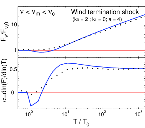
Figure 2: The light curve (upper panel) and the evolution of the temporal decay index $\alpha$ (lower panel) for the synchrotron emission from a spherical relativistic blast wave running into a wind termination shock ($k_{0}=2$, $k_{1}=0$, $a=4$ in Eq. [1]), in the frequency range $\nu<\nu_{m}<\nu_{c}$. Shown are the results of the semi-analytic model described is §2.2 (solid thick blue line) and of the numerical code described in Appendix A (black dots) for a wind termination shock. The semi-analytic result for the same wind without a termination shock (where $\rho_{\rm ext}=A_{0}r^{-k_{0}}$ at all radii; red thin line) is added for reference.

The semi-analytic model for the light curve that has been developed in §2.2 is now applied to a wind termination shock, for which $k_{0}=2$, $k_{1}=0$, and $a=4$. We also compare the results of this semi-analytic model to the numerical model that is described in Appendix A. The resulting light curves are displayed in Figures 2-4 for the three most relevant power law segments (PLSs) of the spectrum. The results of the semi-analytic model nicely agree with the numerical results. Some differences do exist but the qualitative behavior (i.e. variation time scales and amplitudes) is similar, and even the quantitative differences are not very large. The main differences between the semi-analytic model and the numerical simulations are a small initial dip before the rise in the flux for $\nu<\nu_{c}$, a difference in the exact starting time for the change in the temporal decay index for $\nu_{m}<\nu<\nu_{c}$ and $\nu>\max(\nu_{m},\nu_{c})$, and a slightly different normalization of the asymptotic flux at $T\gg T_{0}$ for $\nu<\nu_{c}$. The latter arises since we neglect the dependence of the function $g$ on $k$ in these PLSs ($g$ does not depend on $k$ for $\nu>\nu_{c}$) in the semi-analytic model. This causes a deviation (by a factor of the order of unity) in the normalization of the asymptotic flux calculated by the semi-analytic model, compared to its true value, in cases where $k_{0}\neq k_{1}$.

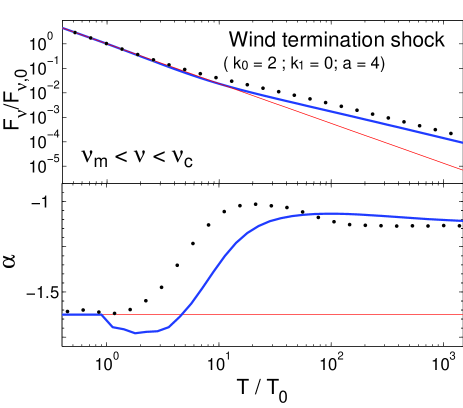
Figure 3: Same as Figure 2 but for the spectral range $\nu_{m}<\nu<\nu_{c}$. We use $p=2.5$.

The light-curves show a smooth transition between the asymptotic power law behavior at $T<T_{0}$ and at $T\gg T_{0}$. There is no rebrightening in PLSs where the flux decays at $T<T_{0}$ ($\nu>\nu_{m}$), and no sharp feature in the light curve which might serve as a clear observational signature. The transition between the two asymptotic curves ($T<T_{0}$ & $T\gg T_{0}$) is continuous with the temporal decay index rising slowly for $\nu<\nu_{c}$ and mildly fluctuating for $\nu>\nu_{c}$. The values of the temporal index $\alpha\equiv d\log F_{\nu}/d\log\nu$ during its rising or fluctuating phase do not exceed its asymptotic value at $T\gg T_{0}$ by more than $0.1$, at any time. Therefore, the only observable signature of a wind termination shock is a continuous break (with $\Delta\alpha=0.5$) below $\nu_{c}$. Above $\nu_{c}$ there is no change in the asymptotic value of the temporal index $\alpha$, and it only slowly fluctuates with a very small amplitude ($\approx 0.1$), which is extremely hard to detect. Note that these results are applicable for a case where the blast-wave remains relativistic also after it encounters the termination shock (i.e. $\gamma_{3}\approx 0.72\gamma_{4}\gtrsim 3$).

The break in the light curve (the shallowing of the flux decay for $\nu_{m}<\nu<\nu_{c}$ or the transition from constant to rising flux for $\nu<\nu_{m}<\nu_{c}$) occurs over about one decade in time. Initially there is very little difference relative to the case where there is no wind termination shock (and $\rho_{\rm ext}=A_{0}r^{-k_{0}}$ at all radii), or even a small dip at $\nu>\max(\nu_{m},\nu_{c})$, while a rise in the relative flux starts at $\tilde{T}=T/T_{0}\sim 2-4$. The light curve approaches its asymptotic late time power law behavior at about $\tilde{T}\sim 10-10^{2}$. This can be understood as follows.

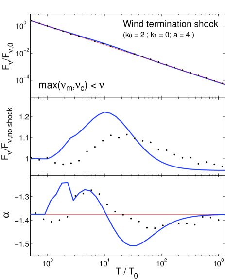
Figure 4: Same as Figure 3 but for the spectral range $\nu>\max(\nu_{m},\nu_{c})$, and with an additional panel for the ratio of the flux with and without a wind termination shock.

The contribution to the observed flux from within a given angle $\theta$ around the line of sight does not change drastically across the density jump. However, there is a sudden decrease in the Lorentz factor of the shocked material behind the forward shock, so that the effective visible region increases from $\theta\lesssim\gamma_{4}^{-1}$ to $\theta\lesssim\gamma_{3}^{-1}=\psi/\gamma_{4}$. This is responsible for most of the observable signature, and it starts affecting the light curve noticeably only when photons emitted just after $R_{0}$ from an angle $\theta\gtrsim\gamma_{4}^{-1}$ arrive to the observer, namely at $\sim T_{\theta}(R_{0,-})=4T_{0}$ where

$$T_{\theta}(R_{0,\pm})\equiv\lim_{\epsilon\to 0}T_{\theta}[(1\pm\epsilon)R_{0}]\ .$$ (23)

This full angular effect becomes apparent when photons from the same radius and an angle of $\theta\sim\gamma_{3}^{-1}$ reach the observer, at $\sim T_{\theta}(R_{0,+})=2(4-k_{0})\psi^{2}T_{0}\approx 8T_{0}$. The radial time is smaller than the angular time, and therefore the radial effect would only slightly increase the time when the total effect becomes prominent. The light curve approaches its asymptotic power law behavior when the dynamics approach the new self similar evolution, at $\sim\tilde{R}_{\rm BM}=2^{1/(3-k_{1})}$. Since $[\gamma_{4}/\gamma(\tilde{R}_{\rm BM})]^{2}\sim 4$ and therefore $\tilde{T}_{\theta}(\tilde{R}_{\rm BM})\sim 16$, while $\tilde{T}_{r}(\tilde{R}_{\rm BM})\sim 2.6$, this corresponds to $\tilde{T}\sim 20$. Obviously, this is a rough estimate, but it agrees reasonably well with the numerical results.

Our main result for the light curves from a wind termination shock is that there is no prominent readily detectable signature in the light curve. This is very different from the results of previous papers that explored a wind termination shock (Ramirez-Ruiz et al., 2001, 2005; Dai & Lu, 2002; Eldridge et al., 2006; Pe’er & Wijers, 2006) which predicted a clear observational signature (including optical rebrightening also when the termination shock is at a sufficiently small radius so that the blast-wave is still relativistic when it runs into it). In some of these works (Ramirez-Ruiz et al., 2001, 2005) the forward shock becomes non-relativistic after hitting the density jump, which might account for some differences compared to our results which are valid for the case when the forward shock remains relativistic after running into the density jump. In other works (Dai & Lu, 2002; Eldridge et al., 2006; Pe’er & Wijers, 2006), however, the forward shock is assumed to remain relativistic after encountering the density jump, similar to our assumption. The main reason for the discrepancy relative to the latter works is that they did not consider either the effect of the reverse shock on the dynamics (Eldridge et al., 2006) or did not properly account for the effect of different photon arrival times from different angles relative to the line of sight from any given radius (Dai & Lu, 2002; Pe’er & Wijers, 2006). Both effects tend to smooth out the resulting variability in the light curve.

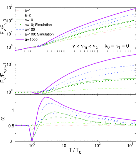
Figure 5: The light curve (upper panel), the ratio of the flux with and without a density jump (middle panel), and the evolution of the temporal index $\alpha$ (lower panel) for the synchrotron emission from a spherical relativistic blast wave propagating into a medium with a step like density profile ($k_{0}=k_{1}=0$ in Eq. [1]), in the frequency range $\nu<\nu_{m}<\nu_{c}$. Shown are the results of the semi-analytic model described is §2.2 for four different density contrasts ($a=2,~{}10,~{}100\;\&\;1000$) and of the numerical code described in Appendix A for two cases ($a=10\;\&\;100$). We use here $p=2.5$.

3.2 Spherical Jump in a Uniform External Medium

Next we explore the light curve that results from a spherical relativistic blast-wave running into a uniform external density with a jump at some radius $R_{0}$ (i.e., $k_{0}=k_{1}=0$ and $a>1$). Such a density profile can be generated, for example, by the contact discontinuity between shocked winds from two evolutionary phases of the massive star progenitor. This configuration also serves as an approximation for a large density clump, and constrains the observational signature from a small density clump (see §4).

Figures 5-7 depict the light curves from our semi-analytic model (described in §2.2) for four different density contrasts ($a=2,\,10,\,100,\,1000$), as well as the results of the numerical simulation (described in Appendix A) for two of these cases ($a=10,\,100$). The agreement between the semi-analytic model and the results of the simulation is satisfactory. In all cases (all the different PLSs and $a$ values) the semi-analytic model qualitatively follows the numerical results and recovers the main features (i.e. the correct time scales and amplitudes of the variations and their derivatives). In most cases the quantitative comparison is also impressive (better than $10\%$). The main differences between the semi-analytic model and the simulation results are the small initial dip before the rise in the flux for $\nu<\nu_{m}<\nu_{c}$ (observed also in the wind-termination sock) and an over-shoot for $a=100$ in this PLS. The semi-analytic model predicts an initial dip for $\nu_{m}<\nu<\nu_{c}$, which also appears, although less prominently, in the results of the numerical simulations.

The main result that emerges from Figures 5-7 is that no sharp features appear in any of the light curves, no matter how high the density contrast (at least as long as $\gamma_{3}=\gamma_{4}/\psi\gg 1$ where $\psi\approx(3a/4)^{1/4}$ for $a\gg 1$). Moreover, the maximal deviation of the temporal decay index, $\alpha$, from its asymptotic value (which is the same for $T<T_{0}$ and $T\gg T_{0}$, since $k_{0}=k_{1}$) is not large ($<1$ in all PLSs at all times), and as we show for $\nu_{m}<\nu<\nu_{c}$ it approaches an asymptotic value at large $a$.

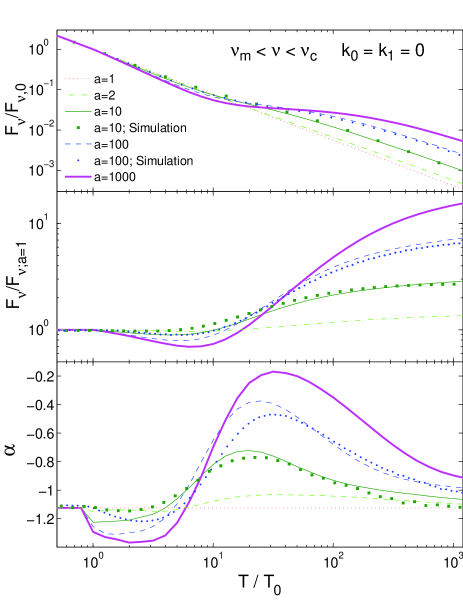
Figure 6: Same as Figure 5 but for the spectral range $\nu_{m}<\nu<\nu_{c}$.

Observationally, the most interesting PLS is $\nu_{m}<\nu<\nu_{c}$, since it typically includes the optical. In this PLS the flux enhancement, $f(T)\equiv F_{\nu}(T)/F_{\nu}(T,a=1)$, is asymptotically $f(T\gg T_{0})=a^{1/2}$, but the transition to this asymptotic value is very gradual. Figure 8 depicts the value of the maximal deviation of the temporal index $\alpha$ from its asymptotic value, $\Delta\alpha_{\rm max}$, as a function of $a$ for two values of $p$. We emphasize the behavior of $\Delta\alpha$ since it is perhaps the easiest quantity to observe. The inability of density fluctuations to produce sharp features in the light curve is demonstrated by the low values of $\Delta\alpha_{\rm max}$ that we find. Some examples are $0.1,~{}0.4~{}(0.35),~{}0.75~{}(0.65)\;\&\;0.95$ for $a=2,~{}10,~{}100\;\&\;1000$, respectively, where the values in brackets correspond to the results of the numerical simulation. Furthermore, for very large values of $a$, $\Delta\alpha_{\rm max}$ saturates at a value of $\approx 1$. Since $\alpha(T<T_{0})=-3(p-1)/4\sim-1$, no rebrightening (i.e., $\alpha>0$) is observed. Moreover, at first (just after $T_{0}$) a mild dip, is apparent in the light-curve. The depth of this dip increases with $a$. Another constraining observable is the time over which $\Delta\alpha_{\rm max}$ is obtained. Thus, we consider the ratio of the time when $\Delta\alpha_{\rm max}$ is obtained and the time when $\Delta\alpha>0$ once it recovers from its initial dip. We find this time ratio to be $\approx 5$ for any reasonable values of $a$ and $p$.

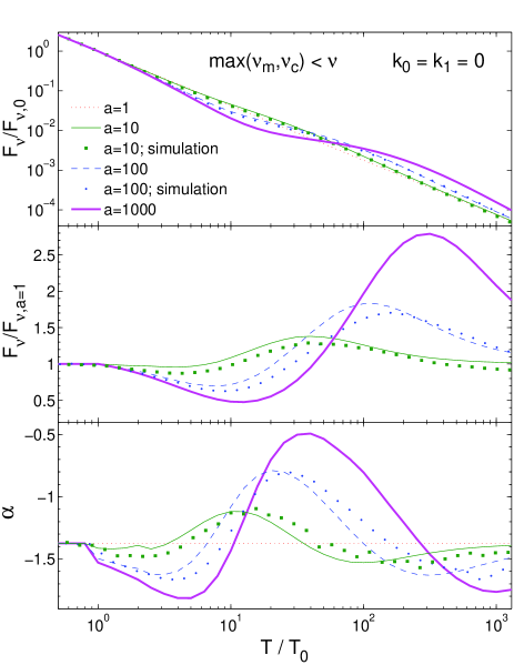
Figure 7: Same as Figure 5 but for the spectral range $\nu_{m},\nu_{c}<\nu$. For clarity we omitted the $a=2$ curve.

Our results can be understood as follows. The contribution to the emission per unit area of the shock front along the line of sight, from a radius $R$ to an observer time $T$, increases with the energy density of the shocked fluid and with its bulk Lorentz factor. A density jump immediately increases the energy density of the freshly shocked fluid (by a factor $a\,\psi^{-2}>1$) while reducing its Lorentz factor (by a factor $\psi^{-1}<1$). The net effect is such that the decrement in the Lorentz factor dominates by a small margin, and the line-of-sight emission actually drops at $R_{0}$. This drop increases with $a$ and is the source of the observed dip right after $T_{0}$. The same drop in $\gamma$ is also the origin of the flux increase that follows. With a lower $\gamma$ the largest angle $\theta$ (from the line of sight) that contributes to the observed emission increases. This contribution becomes apparent only when emission from $\theta\gtrsim 1/\gamma_{4}$ arrives to the observer, at $\sim T_{\theta}(R_{0,-})=8T_{0}$, and is completed when emission from $\theta\gtrsim 1/\gamma_{3}$ is observed, at $\sim T_{\theta}(R_{0,+})=\psi^{2}T_{\theta}(R_{0,-})\sim a^{1/2}T_{\theta}(R_{0,-})$. The transition to the asymptotic value continues up to $T_{\rm BM}\sim a^{1/2}T_{\theta}(R_{0,+})\sim 10aT_{0}$. These time scales explain why the transition is so gradual, and so is the convergence of $\alpha$ to its asymptotic value at $T\gg T_{0}$, for large $a$. Our results show that the maximal value of $\alpha$ is observed around $T_{\theta}(R_{0,+})$, and that for $a\gg 1$, $f[T_{\theta}(R_{0,+})]\approx(0.1-0.4)a^{1/2}$. Now $\Delta\alpha$ can be approximated by $\log\{f[T_{\theta}(R_{0,+})]\}/\log[T_{\theta}(R_{0,+})/T_{\theta}(R_{0,-})]$ which approaches $1$ at large $a$.

It is generally accepted that the main signature of density fluctuations in the external medium are chromatic fluctuations in the afterglow light curve, where sharp features are expected below $\nu_{c}$ (which typically includes the optical bands) and no (or very weak) variability is expected above $\nu_{c}$ (which typically includes the X-rays). This conclusion relies on the fact that a change in the external density effects the asymptotic light-curve (at $T\gg T_{0}$ compared to $T<T_{0}$) only below $\nu_{c}$, but not above $\nu_{c}$. A comparison between Figures 6 & 7 shows that while the behavior in these two PLSs is indeed different, the general concept described above is inaccurate and the differences are more subtle. Both PLSs show smooth fluctuations in the temporal index $\alpha$ with a comparable amplitude. The main difference is in the flux normalization of the asymptotic light curve at $T\gg T_{0}$ compared to $T<T_{0}$. Above $\nu_{c}$ the asymptotic light curve does not change and the observed flux fluctuates around this asymptotic power law decay, while below $\nu_{c}$ the normalization for the asymptotic light curve at $T\gg T_{0}$ is larger than that at $T<T_{0}$ by a factor of $a^{1/2}$, and therefore the flux continuously increase relative to the case where there is no density jump ($a=1$). This type of difference in the behavior is, however, much harder to detect (compared to variations in $\alpha$) since, obviously, the reference light-curve (for $a=1$) cannot be observed.

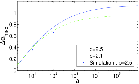
Figure 8: The maximal deviation of the temporal index ($\alpha\equiv d\log F_{\nu}/d\log T$) from its asymptotic value, $\Delta\alpha_{\rm max}$, as a function of the density contrast $a$, for electron power-law indexes $p=2.5$ (solid line) and $p=2.1$ (dashed line). The results of the numerical simulations for $a=10\;\&\;100$ (in which $p=2.5$) are marked as dots.

Several previous works have explored the light curves arising from such a density profile (Lazzati et al., 2002; Dai & Lu, 2002; Nakar, Piran & Granot, 2003; Nakar & Piran, 2003) and all of them predicted much sharper features with an observable rebrightening at $\nu_{m}<\nu<\nu_{c}$ (i.e. $\alpha>0$) which does not exist in the results presented here. In several works (Lazzati et al., 2002; Nakar, Piran & Granot, 2003; Nakar & Piran, 2003) the main cause for the discrepancy is that the effect of the reverse shock on the dynamics was neglected. As we show here, even if the reverse shock in only mildly relativistic ($a\sim 2$), its effect on the dynamics cannot be neglected. The reason for this is that even if the emission from the reverse shock itself is negligible, the abrupt drop in $\gamma$, which is the Lorentz factor of the shocked material behind both the reverse and the forward shocks, prevents very significant variations in $\alpha$ also from the forward shock emission. Dai & Lu (2002) included a partial consideration of the reverse shock, however they neglected the strong effect that angular smoothing has on the light curve.

3.3 The Effects of Proximity to a Break Frequency

So far we have assumed that the observed frequency $\nu$ is very far from the break frequencies ($\nu_{m}$ and $\nu_{c}$) and therefore remains in the same power law segment (PLS) of the synchrotron spectrum throughout the hydrodynamic transitions that we have investigated. Under that assumption the flux density normalized by its value at $T_{0}$ is independent of frequency within each PLS. In this subsection we examine the effect on the light curve if the observed frequency is in the vicinity of a break frequency around the time of the hydrodynamic transition. For this purpose we use our numerical code and consider the cases that have been studied numerically in §3.1 (a wind termination shock) and in §3.2 (a spherical density jump by a factor of $a=10$ or $a=100$ in a uniform medium).

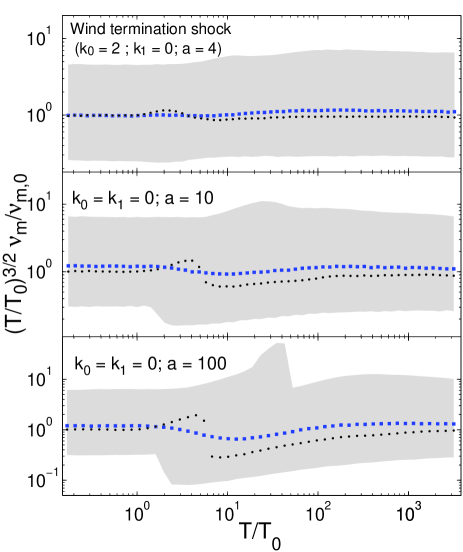
Figure 9: The temporal evolution of the typical synchrotron frequency $\nu_{m}$ (dotted line), which is defined as the frequency at which the spectral index $\beta$ is midway between its value at $\nu\ll\nu_{m}$ ($\beta_{1}=1/3$) and at $\nu\gg\nu_{m}$ [$\beta_{2}=(1-p)/2$], $\beta=(\beta_{1}+\beta_{2})/2$. We use $p=2.5$. The shaded region shows the frequency range where 80% of the change in $\beta$ occurs (between 10% and 90% of $\Delta\beta=\beta_{1}-\beta_{2}$). The frequency where the asymptotic power laws well above and below $\nu_{m}$ meet is marked with filled squares. For clarity, all frequencies are normalized by $\nu_{m,0}=\nu_{m}(T_{0})$ and multiplied by the appropriate power of $\tilde{T}=T/T_{0}$ which takes out the asymptotic time dependence of $\nu_{m}$ at early and late times. The different panels are for different spherical density profiles with a sharp density jump that have been studied in §3.1 – a wind termination shock (upper panel), and in §3.2 – a spherical density jump by a factor of $a=10$ (middle panel) and $a=100$ (lower panel) in a uniform medium.

Figures 9 and 10 show the temporal evolution of the spectral break frequencies $\nu_{m}$ and $\nu_{c}$, respectively, around the time of the density jump. The break frequencies are defined as $\nu_{b}=\min\{\nu|\beta(\nu)<0.5\beta_{1}+0.5\beta_{2}\}$, where $\beta_{1}$ and $\beta_{2}$ are the asymptotic values of the spectral index $\beta$ at $\nu\ll\nu_{b}$ and $\nu\gg\nu_{b}$, respectively, and $b=m,\,c$. The shaded region shows the frequency range $\nu_{10\%}<\nu<\nu_{90\%}$ where $\nu_{10\%}=\min\{\nu|\beta(\nu)<0.9\beta_{1}+0.1\beta_{2}\}$ and $\nu_{90\%}=\max\{\nu|\beta(\nu)>0.1\beta_{1}+0.9\beta_{2}\}$, i.e. where 80% of the change in $\beta$ across the spectral break occurs.

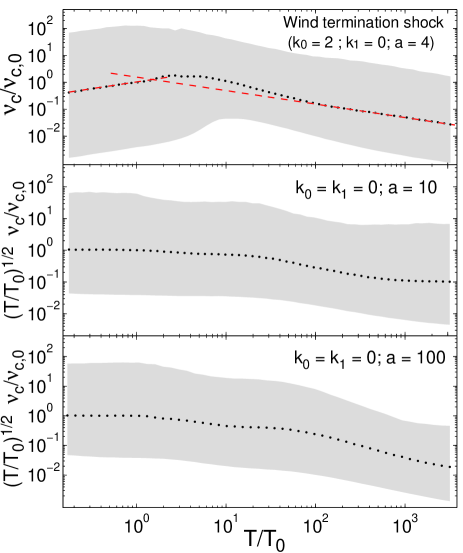
Figure 10: The temporal evolution of the cooling break frequency, $\nu_{c}$, in the same format as Figure 9; here $\beta_{1}=(1-p)/2$, $\beta_{2}=-p/2$, and again $p=2.5$. For a wind termination shock (upper panel) the asymptotic temporal index at $T<T_{0}$ ($\alpha_{1}=1/2$; left dashed line) is different from that at $T\gg T_{0}$ ($\alpha_{2}=-1/2$; right dashed line), and therefore the normalized frequencies are not multiplied by $(T/T_{0})^{1/2}$ as in the other two panels (that are for a density jump in a uniform medium for which $\alpha_{1}=\alpha_{2}=-1/2$).

The typical synchrotron frequency $\nu_{m}$ fluctuates around its asymptotic $T^{-3/2}$ power law decay, which does not depend on the power law index $k$ of the external density. Furthermore, even for a wind termination shock there is no observable change in the asymptotic normalization (i.e. the asymptotic value of $T^{3/2}\nu_{m}$) and only a very small change in the width of the spectral break which is depicted by the shaded region (in agreement with the semi-analytic results of Granot & Sari, 2002). For a density jump in a uniform medium there is no change in the asymptotic normalization or in the asymptotic shape of the spectral break, again as expected from analytic calculations. Both the amplitude and the typical time scale of the fluctuations in $T^{3/2}\nu_{m}$ increase with the density contrast $a$, where the amplitude scales roughly as $a^{1/2}$ and the time scale is roughly linear in $a$. There is a sharp feature in $\nu_{m}$ which occurs first for $\nu_{m,10\%}$, then for $\nu_{m}$, and finally for $\nu_{m,90\%}$. This can be understood as follows. Immediately after the forward shock encounters the density jump $\nu_{m}$ decreases in region 2 and increases in region 3, by a factor of $\sim a^{1/2}$ in both cases. Therefore, as long as the region 3 contributes significantly to the observed spectrum, the break is a superposition of two peaks (corresponding to $\nu_{m,2}$ and $\nu_{m,3}$), separated by a factor of $\sim a$ in frequency, and thus its width increases significantly. Moreover, it causes $\beta(\nu)$ to be non-monotonic, and the definitions of $\nu_{m,10\%}$, $\nu_{m}$, and $\nu_{m,90\%}$ cause these frequencies to have a finite jump when the extremum in $\beta(\nu)$ crosses the appropriate value of $\beta$, which occurs later for higher frequencies. Given the complex structure of the spectral break around $\nu_{m}$ we also present in figure 9 the evolution of the frequency where the asymptotic power laws well above and below the break meet (which can serve as an alternative definition for the location of the break frequency, as was done in Granot & Sari, 2002). This frequency evolves very smoothly and shows very mild fluctuations in all cases, since it is less effected by the transient broadening of the spectral break during the hydrodynamic transition.

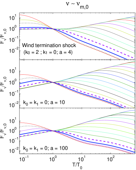
Figure 11: The light curves for frequencies that are in the vicinity of $\nu_{m}$ at the time of the density jump, for the same hydrodynamic transitions that are shown in Figure 9 (with $p=2.5$). The solid thick line is for $\nu\approx\nu_{m}(T_{0})$, the dashed thick line is for $\nu\approx\nu_{m,10\%}(T_{0})$, and the dotted thick line is for $\nu\approx\nu_{m,90\%}(T_{0})$. The remaining curves are spaced by a factor of 2.5 in frequency in the middle panel and 3 in the top and bottom panels.

The evolution of the cooling break frequency, $\nu_{c}$, is shown in Figure 10. For a wind termination shock the temporal index $\alpha$ has different asymptotic values at $T<T_{0}$ ($\alpha_{1}=1/2$) and at $T\gg T_{0}$ ($\alpha_{2}=-1/2$); $\nu_{c}$ transitions rather smoothly between these two asymptotic limits, with a slight overshoot (i.e. $d\log\nu_{c}/d\log T$ dips below $-1/2$) due to the increase in density across the jump (the asymptotic value of $\nu_{c}$ decreases with increasing density). The asymptotic behavior of $\nu_{c}$ is marked with dashed lines showing that for practical purposes (e.g., analytic calculation) it can be well approximated as a sharp temporal transition between $\alpha 1$ and $\alpha_{2}$ at $T\approx 1.5T_{0}$, while keeping in mind that the spectral break itself is very smooth at any time. For a density jump in a uniform medium the asymptotic value of the temporal index does not change ($\alpha_{1}=\alpha_{2}=-1/2$), but the asymptotic normalization of $T^{1/2}\nu_{c}$ at $T\gg T_{0}$ is a factor of $a$ lower than at $T<T_{0}$. The transition between the two asymptotic limits is fairly smooth. The shaded region which corresponds to 80% of the change in $\beta$ across the break is significantly larger for $\nu_{c}$ compared to $\nu_{m}$, corresponding to a smoother break, in agreement with semi-analytic calculations (Granot & Sari, 2002). The transition to the late time asymptotic behavior stretches over a larger factor in time, which increases with $a$.

Figures 11 and 12 show light curves for frequencies that are in the proximity of $\nu_{m}$ and $\nu_{c}$, respectively, around the time of the density jump. There is a smooth transition between the light curves for frequencies that are well below the break frequency and those for frequencies well above the break frequency around the time of the density jump. Our main conclusions from sections §§3.1 and 3.2 remain valid also when the observed frequency is near a break frequency around the time of the density jump. In particular, there is no rebrightening at $\nu\gg\nu_{m}$, and the observed features in the light curve are very smooth. Therefore, our main results are rather robust.

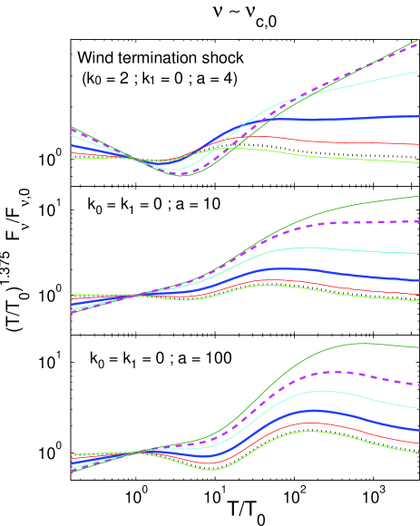
Figure 12: The light curves for frequencies near $\nu_{c}$ at the time of the density jump, for the same hydrodynamic transitions that are shown in Figure 10 (with $p=2.5$). The normalized flux is multiplied by $(T/T_{0})^{(3p-2)/4}\to\tilde{T}^{1.375}$ in order to eliminate asymptotic time dependence at $T\gg T_{0}$ for a uniform medium. The solid thick line is for $\nu\approx\nu_{c}(T_{0})$, the dashed thick line is for $\nu\approx\nu_{c,10\%}(T_{0})$, and the dotted thick line is for $\nu\approx\nu_{c,90\%}(T_{0})$. The remaining curves are spaced by a factor of $\approx 15$ in frequency in the top panel and $\approx 8$ in the middle and bottom panels.

4 A Clump in the External Density

In this section we estimate the effect of a clump in the external density on the light curve. By a clump we refer to a well localized region of typical size $l_{\rm cl}$ which is overdense by a factor of $a>1$ relative to the uniform background external density. For a given clump size $l_{\rm cl}$ and overdensity $a$ (well within the clump, near its center) the effect on the light curve is expected to be larger if the clump has sharper edges, i.e. the smaller the length scale $\Delta l$ over which the density rises by a factor of $\approx a$ relative to the background density. While in practice one might, in many cases, expect $\Delta l\sim l_{\rm cl}$, we consider the limit of a sharp edged clump with $\Delta l\ll l_{\rm cl}$, in order to maximize the effect on the light curve.

Because of relativistic beaming, most of the contribution to the observed light curve from a given radius $R$ is from within an angle of $\theta\lesssim\gamma^{-1}$ around the line of sight, which corresponds to a lateral size of $\sim R/\gamma$. Therefore, a clump in the external density of size $l_{\rm cl}\gg R/\gamma$ would not differ considerably from a spherically symmetric density jump that was considered in §2. If the surface of the clump is not normal to the line of sight (e.g. if the line of sight to the central source does not pass through the center of a spherical clump), this is expected to reduce the effect of the clump on the light curve (similar to what is expected if the clump does not have very sharp edges, $\Delta l\sim l_{\rm cl}$ rather than $\ll l_{\rm cl}$). Therefore the results of §2 can be viewed as a rough upper limit on the effect of “big” clumps ($l_{\rm cl}>R_{0}/\gamma_{3}$). Small to intermediate clumps, of size $l_{\rm cl}\lesssim R_{0}/\gamma_{3}$ are expected to have a smaller effect on the light curve and are investigated below.

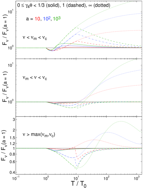
Figure 13: The ratio of the flux with and without a density jump at $R>R_{0}$, within a finite angle $\theta<\theta_{\rm max}$ around the line of sight, for three different density contrasts ($a=10,\,100,\,1000$) and three different angular sizes ($\gamma_{4}\theta_{\rm max}=1/3,\,1,\,\infty$). This serves as an approximate upper limit for the effect of a clump in the external medium on the light curve. The different panels are for the most relevant power law segments of the synchrotron spectrum.

The results of the previous section, and in particular the semi-analytic model for the light curve that was derived in §2.2, can be used to put an approximate upper limit on the effect that a density clump could have on the observed light curve. Such a limit is achieved by using the spherical model from §2.2 within a finite solid angle: $\theta_{\rm min}<\theta<\theta_{\rm max}$ and $\phi_{\rm min}<\phi<\phi_{\rm max}$ in spherical coordinates, while in the radial direction the clump extends out to $R\gg R_{0}$. In practice we expect the radial extent of the clump to be $\Delta R\sim l_{\rm cl}$, similar to its extent in the $\theta$ direction ($\sim R_{0}\Delta\theta$ where $\Delta\theta=\theta_{\rm max}-\theta_{\rm min}$) and in the $\phi$ direction ($\sim R_{0}\bar{\theta}\Delta\phi$ where $\Delta\phi=\phi_{\rm max}-\phi_{\rm min}$ and $\bar{\theta}=[\theta_{\rm min}+\theta_{\rm max}]/2$). In our coarse approximation the clump has no upper bound in the radial direction, and its lateral size scales linearly with radius. Obviously, this sets an (approximate) upper limit for the effect on the light curve of a clump with a size $l_{\rm cl}$ in all directions (which is roughly given by $l_{\rm cl}\sim R_{0}\Delta\theta\sim R_{0}\bar{\theta}\Delta\phi\sim\Delta R$ in spherical coordinates).

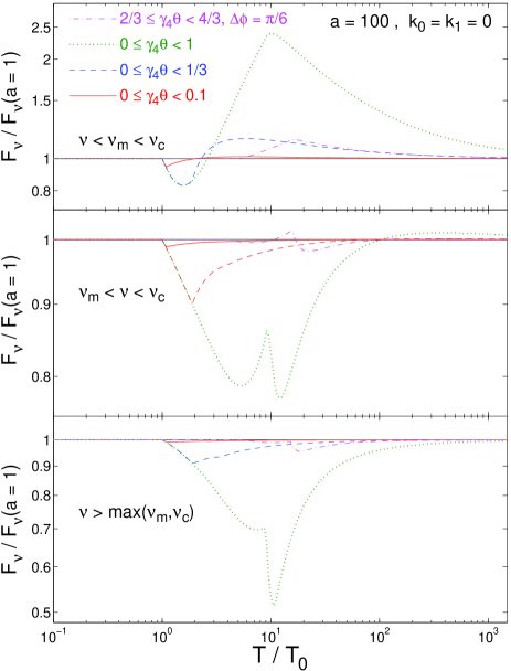
Figure 14: Similar to Figure 13 but for a fixed density contrast, $a=100$, and for three clumps along the line of sight together with a clump that is at the side of the visible region at the time of collision, centered around $\gamma_{4}\theta\approx 1$.

Figure 13 shows the results of this model for a density clump that lies along the line of sight, $\theta_{\rm min}=0$ and $\gamma_{4}\theta_{\rm max}=1/3,\,1,\,\infty$ while $\Delta\phi=2\pi$, for three different values of the density contrast ($a=10,\,100,\,1000$) and for the three most relevant power law segments of the spectrum (that were modeled in §2.2). The smaller the angular extent of the clump, the smaller the amplitude of the change in the flux relative to its value for the smooth underlying density distribution without the clump ($a=1$), and the smaller the factor in time over which it effects the flux significantly (e.g., the full width at half maximum of the relative flux). This behavior is expected since both the amplitude and the duration of the fluctuation depends on the size of the clump (Ioka, Kobayashi & Zhang, 2005). The amplitude depend on the ratio in size between the perturbed region (of length scale $l_{cl}$) and the unperturbed region (of length scale $R/\gamma$) of the blast wave, and thus increase with $l_{cl}$. The duration depends on the delay in the arrival time of photons emitted from the perturbed region, which again increase with the size of this region.

As can be seen in Figure 13, the amplitude of the fluctuation in the relative flux increases with the density contrast $a$. There is a sharp transition in the light curve at $\tilde{T}=1+2(4-k_{0})(\gamma_{4}\theta_{\rm max})^{2}$, when the radiation from the outer edge of the clump at $R=R_{0}$ reaches the observer, which corresponds to the peak in the relative flux for $\gamma_{3}\theta_{\rm max}=\gamma_{4}\theta_{\rm max}\psi^{-1}\sim 1$. Such sharp features (see also Figure 14) are caused by the over-simplified clump model that we use here, and are expected to be smoothed out in more realistic models of clumps. Above $\nu_{m}$ a clump can produce a dip or a bump in the relative flux with a relatively small amplitude (depending on its size and density contrast), while below $\nu_{m}$ it produces a bump in the relative flux with a larger amplitude.

Figure 14 shows the relative flux for a fixed density contrast, $a=100$, for three clumps along the line of sight with different angular sizes ($\Delta\phi=2\pi$, $\theta_{\rm min}=0$ and $\gamma_{4}\theta_{\rm max}=0.1,\,1/3,\,1$), as well as for a clump close to the edge of the visible region at the time of the collision, $\gamma_{4}(\theta_{\rm min},\theta_{\rm max})=(2/3,4/3)$ and $\Delta\phi=\pi/6$, which occupies the same solid angle as the clump along the line of sight with $\gamma_{4}\theta_{\rm max}=1/3$. The effect of a given clump on the light curve is maximal when it is along the line of sight, and it becomes smaller the further it is from the line of sight (i.e., its effect is significant over a shorter time scale and the amplitude of the change in the relative flux is somewhat reduced).

Overall, a fairly large clump of size $l_{\rm cl}\gtrsim R/\gamma$ with a sufficiently large density contrast ($a\gtrsim 10-10^{2}$) is required in order to produce an observable signature in the light curve, and even then the most prominent signal would be below $\nu_{m}$, which is typically relevant for the radio. In the optical, which is typically above $\nu_{m}$, there would only be a small dip or bump in the relative flux, which would be hard to detect.

5 Implications to GRBs 021004, 000301C, 030329 and SHB 060313

Next we reconsider the cause for the fluctuations in the optical afterglow light curves of the long-soft GRBs 021004, 000301C, and 030329, as well as the very recent short-hard GRB 060313, in light of our results. GRB 021004 showed significant variability in its optical afterglow (Pandey et al., 2002; Fox et al., 2003; Bersier et al., 2003; Uemura et al., 2003) which included three distinct episodes of mild rebrightening ($\alpha\gtrsim 0$) at $T\sim 0.05\;$days, $\sim 0.8\;$days, and $\sim 2.6\;$days. Just before the first of these epochs, $\alpha\sim-0.7$, and it then became positive over a factor of $\sim 2-3$ in time. Such a large increase in $\alpha$ over a relatively small factor in time is hard to accommodate by a jump in the external density: $\Delta\alpha\sim 1$ requires $a\gtrsim 10^{2}$ and even then it is hard to achieve such an increase in $\alpha$ over a factor of $\sim 2-3$ in time. The second rebrightening episode lies within the tail of the first, and is therefore not a very “clean” case to study. The third rebrightening epoch at $\sim 2.6\;$days is somewhat more isolated, and has $\Delta\alpha\gtrsim 1$ where most of the increase in $\alpha$ is within about a factor of $\sim 1.5$ in time. This is extremely hard to achieve by variations in the external density. On the other hand, angular fluctuations in the energy per solid angle within the jet (a “patchy shell”) nicely account for both the fluctuations in the light curve and the variability in the linear polarization of this afterglow (Granot & Königl, 2003; Nakar & Oren, 2004).

GRB 000301C displayed a largely achromatic bump in its optical to NIR light curves (Sagar et al., 2000; Berger et al., 2000) peaking at $T\sim 3.8\;$days. Before the bump $\alpha\approx-(1.2-1.3)$ and during the rise to the bump $\alpha$ became slightly positive, so that $\Delta\alpha\sim 1.5$, where most of the increase in $\alpha$ occurred over a factor of $\sim 1.5$ in time. We find that this cannot be produced by a sudden change in the external density (as has been suggested by Berger et al., 2000). The decay just after the peak of the bump is very sharp, $\alpha\approx-(3.5-4)$, and since $\beta-\alpha>2$ (Sagar et al., 2000, find $\beta=-0.96\pm 0.08$ during the decay just after the peak, at $T=4.8\;$days) this requires a deviation from spherical symmetry (Kumar & Panaitescu, 2000), and might not be easy to achieve with angular fluctuations in the energy per solid angle within the jet (a “patchy shell”) or aspherical refreshed shocks. In this case an alternative microlensing interpretation (Garnavich, Loeb & Stanek, 2000) was shown to be able to nicely reproduce the shape of the bump (Gaudi, Granot & Loeb, 2001).

GRB 030329 has one of the best monitored and densely sampled optical afterglow light curves to date. It is presented in great detail by Lipkin et al. (2004) who clearly show that the light curve contains several rebrightening ($\alpha>0$) episodes in which $\Delta\alpha>2$. All of these episodes have a similar structure and occur over a small factor in time ($\Delta T<T$). In previous works it has been suggested that some of these rebrightening episodes are a result of density fluctuations. Pe’er & Wijers (2006) have suggested that the first (and largest) rebrightening episode is the signature of a wind termination shock. Sheth et al. (2003) have followed Berger et al. (2003) in attributing the first rebrightening episode to a two-component jet, but argued that the subsequent rebrightening episodes could be explained by variations in the external density. Our results clearly show that none of the bumps in the optical light curve of GRB 030329 can be a result of density bumps. This implies that the two-jet model of Berger et al. (2003) and Sheth et al. (2003) fails to account for most of the observed light-curve fluctuations. Excluding density fluctuations as the possible source of any of the major bumps, together with the similarity in the shapes of the bumps (Lipkin et al., 2004), support a sequence of similar episodes in which the energy of the jet fluctuates, such as a late time energy injection by “refreshed shocks” (Granot, Nakar & Piran, 2003).

The afterglow of the very recent short-hard GRB 060313 has been monitored both by the X-ray telescope (XRT) and by the optical/ultra-violate telescope (UVOT) on board Swift (Roming et al., 2006). The optical/UV light curve showed three sharp bumps/flares at $T\sim 1.7\;$hr, $\sim 3.2\;$hr, and $\sim 6.6\;$hr, with an amplitude of more than a factor of 2 in flux and a very short rise time of $\Delta T\lesssim 0.1T$. During the same time the X-ray light curve showed a smooth (and steeper) power law decay. This was interpreted by Roming et al. (2006) as the result of variations in the external density by a factor of $\sim 2$, where the lack of variability in the X-rays was attributed to $\nu_{c}$ being between the optical/UV and the X-rays. Our results clearly show that such sharp rebrightening episodes as were seen in the optical/UV afterglow light curve of GRB 060313 cannot be the result of variations in the external density. Therefore, there must be some other cause for this variability, such as late time internal shocks with a very soft spectrum, as was suggested by Roming et al. (2006) as an alternative mechanism.

6 Conclusions

We have presented a semi-analytic model for the light-curve resulting from synchrotron emission by a spherical relativistic blast-wave that propagates into a power law external density profile with a single sharp density jump at some radius $R_{0}$. Our solution is general enough to include a transition in the density power-law index ($k$) at $R_{0}$, but is limited to cases in which the blast-wave remains relativistic after it encounters the density jump. This model has been used to explore in detail two density profiles that are most relevant to GRB afterglows: a wind termination shock, and a sharp density jump between two regions of uniform density. The latter results are also used to constrain the signature of density clumps in a uniform medium. We have also carried out detailed numerical simulations for several of the cases which we have studied in detail. These numerical results serve three purposes. First, they are used in order to obtain more accurate light curves for the cases which are of special interest. Second, they are appropriate for calculating the light curves in the vicinity of a spectral break frequency (§3.3). Third, they serve as a test for the quality of our simple semi-analytic model, which is found to give a very good qualitative description and reasonable quantitative description of the light curve.

Our main result is that density jumps do not produce sharp features in the light curve, regardless of their density contrast! The results of our specific case studies are as follows.A wind termination shock:

• The light curve shows a smooth transition, which lasts for about one decade in time, between the asymptotic power-law behavior at $T<T_{0}$ and at $T\gg T_{0}$.

• There is no rebrightening or any other sharp feature that can be used as a clear observational signature.

• Above the cooling frequency, $\nu_{c}$, there is no change in the asymptotic value of the temporal index, $\alpha$, and it only fluctuates with a small amplitude ($\Delta\alpha\approx 0.1$).

• The only observable signatures of a wind termination shock are a smooth break, with an increase of $\Delta\alpha=0.5$ in $\alpha$, below $\nu_{c}$ and a transition in the temporal evolution of $\nu_{c}$.

A density jump between two uniform density regions:

• The light curve shows a smooth transition between the two asymptotic power laws (at $T<T_{0}$ and $T\gg T_{0}$).

• The transition time increases with the density contrast, $a$, and is about $\sim 10aT_{0}$.

• The maximal deviation, $\Delta\alpha_{\rm max}$, of the temporal index $\alpha$ from its asymptotic value (at $T<T_{0}$ and $T\gg T_{0}$) is small. For example, $\Delta\alpha_{\rm max}(a=10)<0.4$; $\Delta\alpha_{\rm max}$ depends weakly on $a$ and approaches $\approx 1$ at very large $a$ values. Therefore, a density jump cannot produce an optical rebrightening when $\nu_{\rm optical}>\nu_{m}$.

• The light curve fluctuates also above $\nu_{c}$ (typically including the X-ray band). While the asymptotic flux (at $T\gg T_{0}$) above $\nu_{c}$ is unaffected by the density jump, the fluctuations in $\alpha$ are comparable to those below $\nu_{c}$.

An overdense clump on top of a uniform density background:

• Only a fairly large clump ($l_{\rm cl}\gtrsim R/\gamma$) with a sufficiently large density contrast ($a\gtrsim 10-10^{2}$) produces a significant fluctuation in the light curve.

• The effect of a clump on the light curve is significantly larger when it is located along the line of sight, than at an angle of $\sim 1/\gamma$ from the line of sight.

• The signature of a clump is most apparent at $\nu<\nu_{m}<\nu_{c}$.

• Above $\nu_{m}$ a clump can actually cause a small dip in the light curve, while below $\nu_{m}$ it causes a (larger) bump.

For a spherical density jump our conclusions are based on accurate results, while in the case of a density clump we obtain only an approximate upper limit for its effect on the light-curve. Therefore, our results for density clumps should be taken only as rough guidelines. Our main results remain valid also when the observed frequency is close to a spectral break frequency around the time of the density jump.

Our conclusions are very different from those of previous works, which predicted a significant optical rebrightening, and rather sharp features in the afterglow light curve. The main cause for this difference is our careful consideration of both the effect of the reverse shock on the dynamics (which we find cannot be neglected even when $a\sim 2$), and the arrival time of the photons to the observer from different parts of the emitting regions. Both of these effects tend to smoothen the light curve significantly.

Finally, we considered the implications of our results for the origin of the fluctuations in the highly variable light curves of four GRBs (3 long-soft GRBs and one short-hard GRB). We find that density variations are unlikely to be the source of the fluctuations in any of these bursts.

We thank Enrico Ramirez-Ruiz, Avishay Gal-Yam, Eran Ofek, Brad Cenko and Pawan Kumar for useful comments. This research was supported by a senior research fellowship from the Sherman Fairchild Foundation (E. N.) and by US Department of Energy under contract number DE-AC03-76SF00515 (J. G.).

Appendix A A One Dimensional Special Relativistic Hydrodynamics and Radiation Code

In order to obtain accurate light curves while relying on a minimal number of approximations we use a one dimensional special relativistic hydrodynamic code and combine it with an optically thin synchrotron radiation module. This is the same code that was used before in Nakar & Piran (2004). We use a one dimensional hydrodynamic code that was generously provided to us by Re’em Sari and Shiho Kobayashi. It is a Lagrangian code based on a second-order Gudanov method with an exact ultra-relativistic Riemann solver and it is described and used in Kobayashi et al. (1999) and Kobayashi & Sari (2000). On top of this code we have constructed a module that calculates the resulting optically thin synchrotron radiation. The code does not include the synchrotron self-absorption or synchrotron self-Compton processes. The effect of the radiation on the hydrodynamics is neglected. Below we describe the physics that is included in the radiation module.

Having the full hydrodynamic evolution of the fluid (from the hydrodynamic code) we first identify the time steps in which a given fluid element is shocked by finding episodes of increase in its entropy. The same fluid element can be shocked many times. Once a fluid element is shocked all its electrons are assumed to be instantly accelerated into a power-law energy distribution with an index $p$, $dN/d\gamma_{e}\propto\gamma_{e}^{-p}$ for $\gamma_{e}>\gamma_{\rm min}$. The energy in the electrons is taken as a constant fraction, $\epsilon_{e}$, of the internal energy, and this condition determines $\gamma_{\rm min}$ (it is assumed that $p>2$). From this point on, and until the same fluid element is shocked again, the electron energy distribution decouples from the internal energy and evolves through radiative cooling and adiabatic cooling or heating ($PdV$ work). The magnetic energy in each fluid element is taken to be a constant fraction, $\epsilon_{B}$, of the internal energy at all times.

One of the main difficulties in calculating the synchrotron radiation at high frequencies is the short cooling time, which may be much shorter than the hydrodynamic time steps. In order to overcome this difficulty, we calculate the radiation during any hydrodynamic time step analytically, in the following way. Immediately after a fluid element crosses a shock, its initial electron energy distribution is taken to be a power-law (with index $p$) between $\gamma_{\rm min}$ and $\gamma_{\rm max}=\infty$. The total emissivity of the fluid element at a given frequency in its own rest frame, during a time step, is obtained by integrating the spectral power of individual electrons over the evolving electron distribution, where each electron is tagged by the value of its initial Lorentz factor. The emission of each electron is obtained by time integration over its instantaneous emissivity, which in turn depends on the evolution of its Lorentz factor (and thus on its initial Lorentz factor) during the time step. This evolution is calculated by considering its radiative losses and its adiabatic cooling or heating. In particular, we calculate the evolution of an electron with initial Lorentz factor $\gamma_{\rm min}$ and of an electron with initial Lorentz factor $\gamma_{\rm max}$. Their values at the end of the time step are taken as the initial values for the next step in which the initial distribution of electrons Lorentz factors is taken again as a power-law between the new values of $\gamma_{\rm min}$ and $\gamma_{\rm max}$. From the point where $\gamma_{\rm max}$ becomes comparable to $\gamma_{\rm min}$ (within a factor of 2) the electron energy distribution is taken as a delta function.

Since we use a one dimensional code in spherical coordinates, which explicitly assumes spherical symmetry, each fluid element represents a thin spherical shell. Once the rest frame spectral power of a fluid element is calculated, we integrate over the contribution of this shell to the observed flux at a given observer time and observer frequency. This calculation takes into account the appropriate Lorentz transformation of the radiation field and photon arrival time from each point along the shell.

References

- Baltz & Hui (2005) Baltz, E. A., & Hui, L. 2005, ApJ, 618, 403
- Berger et al. (2000) Berger, E., et al. 2000, ApJ, 545, 56
- Berger et al. (2003) Berger, E., et al. 2003, Nature, 426, 154
- Bersier et al. (2003) Bersier, D., et al. 2003, ApJ, 584, L43
- Blandford & McKee (1976) Blandford, R. D., & McKee, C. F. 1976, Phys. Fluids, 19, 1130
- Burrows et al. (2005) Burrows, D. N., et al. 2005, Science, 309, 1833
- Covino (2003) Covino, S., Ghisellini, G., Lazzati, D., & Malesani, D. 2003a, in Gamma-Ray Bursts in the Afterglow Era — Third Workshop, ed. L. Piro & M. Feroci (San Francisco: ASP), in press (astro-ph/0301608)
- Dai & Lu (2002) Dai, Z. G., & Lu, T. 2002, ApJ, 565, L87
- Eldridge et al. (2006) Eldridge, J. J., Genet, F., Daigne, F., & Mochkovitch, R. 2006, MNRAS, 367, 186
- Falcone et al. (2006) Falcone, A. D. et al. 2006, to appear in the proceedings of the 16th Annual October Astrophysics Conference in Maryland ”Gamma Ray Bursts in the Swift Era” (astro-ph/0602135)
- Fox et al. (2003) Fox, D. W., et al. 2003, Nature, 422, 284
- Fryer, Rockefeller & Young (2006) Fryer, C. L., Rockefeller, G., & Young, P. A. 2006, preprint (astro-ph/0604432)
- Garnavich, Loeb & Stanek (2000) Garnavich, P. M., Loeb, A., & Stanek, K. Z. 2000, ApJ, 544, L11
- Gaudi, Granot & Loeb (2001) Gaudi, B. S., Granot, J., & Loeb, A. 2001, ApJ, 561, 178
- Gorosabel et al. (2006) Gorosabel, J., Castro-Tirado, A. J., Ramirez-Ruiz, E., Granot, J., et al. 2006, ApJ, 641, L13
- Granot & Königl (2003) Granot, J., & Königl, A. 2003, ApJ, 594, L83
- Granot, Nakar & Piran (2003) Granot, J., Nakar, E., & Piran, T. 2003, Nature, 426, 138
- Granot & Sari (2002) Granot, J., & Sari, R. 2002, ApJ, 568, 820
- Harrison et al. (2001) Harrison, F. A., et al. 2001, ApJ, 559, 123
- Heyl & Perna (2003) Heyl, J. S., & Perna, R. 2003, ApJ, 586, L13
- Ioka, Kobayashi & Zhang (2005) Ioka, K., Kobayashi, s., & Zhang, B. 2005, ApJ, 631, 429
- Kobayashi et al. (1999) Kobayashi, S., Piran, T., & Sari, R. 1999, ApJ, 513, 669
- Kobayashi & Sari (2000) Kobayashi, S., & Sari, R. 2000, ApJ, 542, 819
- Kumar & Panaitescu (2000) Kumar, P., & Panaitescu, A. 2000, ApJ, 541, L51
- Kumar & Piran (2000a) Kumar, P., & Piran, T. 2000a, ApJ, 532, 286
- Kumar & Piran (2000b) Kumar, P., & Piran, T. 2000b, ApJ, 535, 152
- Laursen, & Stanek (2003) Laursen, L. T., & Stanek, K. Z. 2003, ApJ, 597, L107
- Lazzati et al. (2002) Lazzati, D., Rossi, E., Covino, S., Ghisellini, G., & Malesani, D. 2002, A&A, 396, L5
- Lipkin et al. (2004) Lipkin, Y. M., Ofek, E. O., Gal-Yam, A., et al. 2004, ApJ, 606, 381
- Matheson et al. (2003) Matheson, T., et al. 2003, ApJ, 599, 394
- Meszaros (2006) Meszaros, P. 2006, Rep. Prog. Phys. in press (astro-ph/0605208)
- Nakar & Oren (2004) Nakar, E., & Oren, Y. 2004, ApJ, 602, L97
- Nakar, Piran & Granot (2003) Nakar, E., Piran, T., & Granot, J. 2003, New Astron., 8, 495
- Nakar & Piran (2003) Nakar, E., & Piran, T. 2003, ApJ, 598, 400
- Nakar & Piran (2004) Nakar, E., & Piran, T. 2004, MNRAS, 353, 647
- Nousek et al. (2006) Nousek, J. A., Kouveliotou, C., Grupe, D., Page, K., Granot, J., Ramirez-Ruiz, E., et al. 2006, ApJ in press (astro-ph/0508332)
- O’brien et al. (2006) O’brien, P. T., et al. 2006, submitted to ApJ (astro-ph/0601125)
- Panaitescu & Kumar (2000) Panaitescu, A., & Kumar, P. 2000, ApJ, 543, 66
- Pandey et al. (2002) Pandey, S. B., et al. 2002, Bull. Astron. Soc. India, 31, 19
- Pe’er & Wijers (2006) Pe’er, A., & Wijers, R. A. M. J. 2006, submitted to ApJ (astro-ph/0511508)
- Piran (2005) Piran, T. 2005, Rev. Mod. Phys., 76, 1143
- Ramirez-Ruiz et al. (2001) Ramirez-Ruiz, E., Dray, L.M., Madau, P., & Tout, C.A. 2001, MNRAS, 327, 829
- Ramirez-Ruiz, Merloni & Rees (2001) Ramirez-Ruiz, E., Merloni, A., & Rees, M. J. 2001, MNRAS, 324, 1147
- Ramirez-Ruiz et al. (2005) Ramirez-Ruiz, E., García-Segura, G., Salmonson, J.D., & Pérez- Rendón, B. 2005, ApJ, 631, 435
- Rees & Mészáros (1998) Rees, M. J., & Mészáros, P. 1998, ApJ, 496, L1
- Rhoads (1999) Rhoads, J. 1999, ApJ, 525, 737
- Roming et al. (2006) Roming, P. W. A., et al. 2006, preprint (astro-ph/0605005)
- Rybicki & Lightman (1986) Rybicki, G. B., & Lightman, A. P. 1986, Radiative Processes in Astrophysics, by George B. Rybicki, Alan P. Lightman, pp. 400. ISBN 0-471-82759-2. Wiley-VCH , June 1986.,
- Sagar et al. (2000) Sagar, R., et al. 2000, Bull. Astron. Soc. India, 28, 499
- Sari & Esin (2001) Sari, R., & Esin, A. A. 2001, ApJ, 548, 787
- Sari & Mészáros (2000) Sari, R., & Mészáros, P. 2000, ApJ, 535, L33
- Sari, Piran & Halpern (1999) Sari, R., Piran, T., & Halpern, J. 1999, ApJ, 519, L17
- Sato et al. (2003) Sato, R., et al. 2003, ApJ, 599, L9
- Sheth et al. (2003) Sheth, K., et al. 2003, ApJ, 595, L33
- Stanek et al. (1999) Stanek, K. Z., et al. 1999, ApJ, 522, L39
- Stanek et al. (2006) Stanek, K. Z., et al. 2006, submitted to ApJL (astro-ph/0602495)
- Uemura et al. (2003) Uemura, M., et al. 2003, PASJ, 55, L31
- Uemura et al. (2004) Uemura, M., et al. 2004, PASJ, 56, S77
- Wang & Loeb (2000) Wang, X., & Loeb, A. 2000, ApJ, 535, 788
- Wijers (2001) Wijers, R. A. M. J. 2001, in Gamma Ray Bursts in the Afterglow Era, ed. E. Costa, Frontera. F. and Hjorth J. (Springer: Berlin) 306
- Zhang et al. (2006) Zhang, B., et al. 2005, ApJ in press (astro-ph/0508321)