Tachyon dark energy models: Dynamics and constraints

Abstract

We explore the dynamics of dark energy models based on a Dirac–Born–Infeld (DBI) tachyonic action, studying a range of potentials. We numerically investigate the existence of tracking behaviour and determine the present-day value of the equation of state parameter and its running, which are compared with observational bounds. We find that tachyon models have quite similar phenomenology to canonical quintessence models. While some potentials can be selected amongst many possibilities and fine-tuned to give viable scenarios, there is no apparent advantage in choosing a DBI scalar field instead of a Klein–Gordon one.

I Introduction

Most dark energy modelling using scalar fields has followed the quintessence paradigm of a slowly rolling canonical scalar field. However, there has been increasing interest in loosening the assumption of a canonical kinetic term. In its most general form, this idea is known as k-essence AMS . A more specific choice is the ‘tachyon’ gib02 , which can be viewed as a special case of k-essence models with Dirac–Born–Infeld (DBI) action chi03 . This kind of scalar field is motivated by string theory as the negative-mass mode of the open string perturbative spectrum, though its use in the dark energy sector is primarily phenomenological. One goal of such studies is to investigate whether there are any distinctive signatures of non-canonical actions available to be probed by observations. For a recent comprehensive review of dark energy dynamics, see Ref. CST .

Tachyon dark energy has been explored by many authors, for example Refs. CGJP ; HL ; BJP ; GST ; CGST ; car06 . Two papers are particularly closely related to the present work. Bagla et al. BJP focussed on two specific choices of tachyon potential, and carried out numerical analysis of the cosmological evolution in order to constrain them against supernova data and the growth rate of large-scale structure. Copeland et al. CGST studied a wider range of potentials, concentrating mainly on analytical inspection of attractor behaviour and the critical point structure without making comparison to specific observations. In this paper, we aim to merge some of the positive features of each analysis, by studying a wide range of potentials and testing them directly against current observational constraints as given in Ref. WM .

The mechanism of slow rolling is the key ingredient in order to get an accelerating evolution driven by a scalar field. Since the DBI action can be expanded to match the Klein–Gordon one in this regime, one does not expect to find radically different features from the traditional quintessence models. However, we point out that, as compared to canonical quintessence, tachyon models require more fine-tuning to agree with observations. This is consistent with the properties of the slow-roll correspondence between the tachyon and an ordinary scalar ben02 ; GKMP .

II Tachyon dark energy models

II.1 Equations of motion

We assume a four-dimensional, spatially-flat Friedmann–Robertson–Walker Universe filled by dust matter (subscript ‘m’), radiation (‘r’) and a minimally coupled homogeneous DBI tachyon $T$ with potential $V(T)$ and dimension $E^{-1}$. For a perfect fluid $n$ with energy density $\rho_{n}$ and pressure $p_{n}$, the barotropic index is $w_{n}\equiv p_{n}/\rho_{n}$. Each fluid component satisfies a continuity equation

$$\dot{\rho}_{n}+3H\rho_{n}(1+w_{n})=0\,,$$ (1)

with $w_{\rm m}=0$ and $w_{\rm r}=1/3$. Here, a dot is derivation with respect to synchronous time and $H\equiv\dot{a}/a$ is the Hubble parameter defined in terms of the scale factor $a(t)$. In the following a subscript 0 will denote quantities evaluated today (at $t_{0}$), when $a(t_{0})=a_{0}=1$. Defining the critical density today as $\rho_{{\rm c}0}\equiv 3H_{0}^{2}/(8\pi G)$ and assuming that gravity obeys an Einstein–Hilbert action, the Friedmann equation reads

$$H^{2} = \varrho_{\text{m}}+\varrho_{\text{r}}+\varrho_{T}\,,$$ (2)

$$\varrho_{\text{m}} = \Omega_{\text{m},0}a^{-3}\,,$$ (3)

$$\varrho_{\text{r}} = \Omega_{\text{r},0}a^{-4}\,,$$ (4)

$$\varrho_{T} = \frac{U(T)}{\sqrt{1-\dot{T}^{2}}}\,,$$ (5)

where $\varrho_{n}\equiv\rho_{n}/\rho_{c0}$, $U\equiv V/\rho_{c0}$, and the time coordinate has been rescaled as $t\to t/H_{0}$ so that $H=1$ today. The tachyon is dimensionless in these units. Note that the $\varrho_{n}$ are the densities normalized to the present value of the critical density, and are not the density parameters. The present density parameters have values $\Omega_{\text{m},0}\approx 0.24$ spe06 and $\Omega_{\text{r},0}\approx 8\times 10^{-5}$.

The tachyon equation of motion is FT

$$\frac{\ddot{T}}{1-\dot{T}^{2}}+3H\dot{T}+\frac{U_{,T}}{U}=0,$$ (6)

where $U_{,T}\equiv dU/dT$. Since $p_{T}=-V\sqrt{1-\dot{T}^{2}}$, the barotropic index for the tachyon is

$$w_{T}=\dot{T}^{2}-1,$$ (7)

which can vary only between $-1$ and $0$ in order for the action to be well defined. When the scalar field slowly rolls down its potential, $|\dot{T}|\ll 1$, it behaves like an effective cosmological constant, $w_{T}\approx-1$. From now on we drop the subscript ‘$T$’ on $w_{T}$.

Since the cosmological evolution spans many orders of magnitude in synchronous time, for numerical work it is convenient to switch to the number of $e$-foldings $N\equiv\ln a/a_{0}=\ln a$ as the evolution parameter, so that

$$\varrho_{\text{m}}=\Omega_{\text{m},0}e^{-3N}\,,\qquad\varrho_{\text{r}}=\Omega_{\text{r},0}e^{-4N}\,.$$ (8)

Derivatives with respect to $N$ will be denoted by primes, so that $\dot{Q}=HQ^{\prime}$ and $\ddot{Q}=H^{2}(Q^{\prime\prime}-\epsilon Q^{\prime})$ for any quantity $Q$, where $\epsilon\equiv-\dot{H}/H^{2}=-(H^{2})^{\prime}/(2H^{2})$. With the compact notation $x\equiv H^{2}$, $\varrho\equiv\varrho_{\text{m}}+\varrho_{\text{r}}$, the Friedmann equation becomes

$$x=\varrho+\frac{U}{\sqrt{1-xT^{\prime 2}}}\,.$$ (9)

The equation of motion for the tachyon is

$$\frac{x(T^{\prime\prime}-\epsilon T^{\prime})}{1-xT^{\prime 2}}+3xT^{\prime}+\frac{U_{,T}}{U}=0\,,$$ (10)

where

$$\epsilon=-\frac{x^{\prime}}{2x}\,,\qquad x^{\prime}=-3\varrho_{\text{m}}-4\varrho_{\text{r}}-\frac{3xUT^{\prime 2}}{\sqrt{1-xT^{\prime 2}}}\,.$$ (11)

From Eq. (10) one finds

$$T^{\prime\prime}=-\frac{1}{x}\left[\frac{x^{\prime}T^{\prime}}{2}+(1-xT^{\prime 2})\left(3xT^{\prime}+\frac{U_{,T}}{U}\right)\right]\,.$$ (12)

Mapping between the number of $e$-foldings and the redshift $z\equiv a_{0}/a-1$, we note that at big bang nucleosynthesis (BBN) $N_{\rm BBN}\approx-20$ ($z\approx 10^{9}$), at matter–radiation equality $N_{\rm eq}\approx-8$ ($z\approx 3200$), and at recombination $N_{\rm rec}\approx-7$ ($z\approx 1100$).

As regards the initial conditions at early times for the dynamical equations, we can consider two qualitative cases. In the first one, the scalar field starts rolling down very slowly, $xT^{\prime 2}\ll 1$. The Friedmann equation becomes linear in $x$ and, during radiation domination, $\varrho\gg U$ and $x\approx\varrho$. In such a picture of the events, the initial condition is a radiation-dominated Universe in which a dynamical cosmological constant is negligible. Later on, $\varrho_{T}$ increases relative to $\varrho_{\rm r}$, eventually dominating at low redshift, while $w$ stays negative and varies, perhaps non-monotonically, from around $-1$ to $w_{0}<0$. The parameters of the model and the shape of the potential can be adjusted so that the actual value of $w_{0}$ is compatible with supernovæ data.

In the second case $xT^{\prime 2}\lesssim 1$, that is, $T^{\prime}$ is large enough to compensate, but not override, $x\gg 1$. The tachyon starts from a dust regime and ends up again with a suitable negative $w_{0}$. This is precisely the situation studied numerically in Ref. CGST for $U\propto T^{-1}$.

Below, we shall focus mainly on the first case, which encodes all the relevant features of the models.

II.2 Tracking and creeping regimes

Quintessence behaviour typically falls into one of two classes, named as tracking and creeping in Refs. SWZ ; WCOS (see also Refs. CL ; lin06 which refer to the more general late-time behaviour in these scenarios as freezing and thawing). The same kind of evolution also occurs in the tachyon case.

Tracking behaviour occurs when the potential has an attractor as a response to a cosmological fluid, which renders the final outcome (at fixed fluid density) independent of the initial conditions. Many potentials support tracking behaviour, which takes place provided the initial dark energy density is not too low (otherwise the scalar field cannot dominate by the present). A tracking field slows down near the present as it starts to feel the friction induced by its own dominance of the energy density, and hence has equation of state reducing with time ($w^{\prime}<0$). Note that an asymptotic solution, in which radiation and matter are negligible and dark energy is the only component, may be an attractor but is not a tracker according to the above definition; tracking behaviour is induced by another fluid component.

A creeping field is one which sits static at low energy density until the density of other materials drops low enough for it to become dynamical and start to move at the present epoch. Creeping dark energy typically does not make predictions independent of initial conditions, but can be characterized by the equation of state increasing away from $-1$ at the present epoch as the field starts to move ($w^{\prime}>0$).

Potentials with tracking regimes also feature creeping behaviour for low enough initial density, which can lead to different predictions from the same potential. Creepers can be seen mainly as models which have passed the attractor and are frozen until they reach it, although creeping behaviour can also be found for many potentials which do not support observable tracking.

In order to regard the tachyon as a model of dynamical dark energy, it is useful to parametrize the barotropic index as a function of the scale factor:

$$w=w_{0}+w_{a}(a-1),$$ (13)

so that $w=w_{0}$ today. Its value can be found by solving the Friedmann equation today for $T^{\prime}_{0}=T^{\prime}(0)$, getting from Eq. (9)

$$w_{0}=(T^{\prime}_{0})^{2}-1=-\left(\frac{U_{0}}{1-\varrho_{0}}\right)^{2}.$$ (14)

From Eq. (10), one has that

$$w_{a} = e^{-N}w^{\prime},$$ (15)

$$w^{\prime} = 2wT^{\prime}\left(3xT^{\prime}+\frac{U_{,T}}{U}\right)\,.$$ (16)

Then one has $w^{\prime}<0$ when either $T^{\prime}<0$ and $3xT^{\prime}+U_{,T}/U<0$ (for inverse power-law potentials, $U\sim T^{-\beta}$, the latter condition is $3xTT^{\prime}-\beta<0$, true when $T>0$), or $T^{\prime}>0$ and $3xT^{\prime}+U_{,T}/U>0$.

The transition between a tracker and a creeper can be defined by imposing an initial condition for $T$ and $T^{\prime}$ so that $w^{\prime}_{0}=0$. Genuinely non-tracking models are problematic as they do not make definite predictions, in the sense that there is strong dependence on initial conditions. This makes them rather unattractive, although by no means ruling them out. Indeed, it makes some of them more viable than trackers in relation to experimental bounds, as we shall see.

II.3 Choice for the tachyon potential

As for the tachyon self-interaction, there are a number of models which one can consider, some being motivated by nonperturbative string theory and others purely by phenomenology. We review the classification of Ref. CGST , to which we refer for further details and references. For each case, past results are summarized. In the following, $U_{c}$ is a normalization constant.

1. $U=U_{c}T^{-\beta}$, $\beta<0$, $\epsilon\propto T^{\beta-2}\to\infty$ as $T\to 0$. This model is affected by instabilities FKS .

2. $U=U_{c}T^{-\beta}$, $0<\beta<2$, $\epsilon\propto T^{\beta-2}\to 0$ as $T\to+\infty$ [asymptotically de Sitter (dS)]. In order to get viable cosmologies, $U_{c}$ does not need to be fine-tuned since it is not affected by the super-Planckian problem of the inverse quadratic potential. In general there is a stable late-time attractor AF . In Ref. CGST the case $\beta=1$ was considered as a numerical example.

3. $U=U_{c}T^{-2}$, $\epsilon={\rm constant}$. This is the potential associated to the exact power-law solution $a=t^{p}$ BJP ; AF ; pad02 . One has to fine-tune $U_{c}$ in order to get sufficient acceleration today. A phase-space analysis in Refs. AL ; CGST confirms that it is difficult for this model to explain dark energy, since the only late-time attractor in the presence of matter or radiation has $\varrho_{T}/x\to 0$.

4. $U=U_{c}T^{-\beta}$, $\beta>2$, $\epsilon\propto T^{\beta-2}\to\infty$ as $T\to+\infty$. This potential has not been studied numerically previously, but Ref. AF showed that it has a dust attractor. The authors of Ref. CGST also argued that it behaves as in model 7 below.

5. $U=U_{c}\exp(1/\mu T)$, $\mu>0$, $\epsilon\propto\exp(-1/\mu T)/T^{2}\to 0$ as $T\to+\infty$. This gives an asymptotic dS solution with effective cosmological constant given by $U_{c}$. This potential has been considered also for Klein–Gordon quintessence ZWS ; SWZ , and it should have properties similar to model 2 CGST .

6. $U=U_{c}\exp(\mu^{2}T^{2})$, $\mu>0$, $\epsilon\propto T^{2}\exp(-\mu^{2}T^{2})\to 0$ as $T\to 0$. This potential arises in KKLT setups KKLT for massive scalar modes on the $D$-brane GST . The field oscillates around $T=0$ with effective cosmological constant given by $U_{c}$, and can give viable scenarios CGST .

7. $U=U_{c}\exp(-\mu T)$, $\mu>0$, $\epsilon\propto\exp(\mu T)\to\infty$ as $T\to+\infty$. This potential arises in $D$–$\bar{D}$ systems of coincident branes with a real tachyonic mode, and was studied in Ref. BJP . The authors of Ref. CGST found it to have a stable dust attractor after a period of acceleration. They suggested the possibility that we are living during this transient regime. Note that this potential is a large-field approximation of $U=U_{c}/\cosh(\mu T)$ LLM .

8. $U=U_{c}\exp(-\mu^{2}T^{2})$, $\mu>0$, $\epsilon\propto T^{2}\exp(\mu^{2}T^{2})\to\infty$ as $T\to+\infty$. In Ref. CGST it was argued that its predictions are similar to model 7.

These potentials offer a rather comprehensive range of generic behaviours: one reaches a cosmological constant regime at infinite time [$U\propto\exp(T^{-1})$], one at finite time ($U\propto\exp T^{2}$), while in other situations the potential asymptotically vanishes.

The structure of analytic asymptotic solutions of the equations of motion for inverse power-law and exponential potentials is presented in the Appendix.

III Numerical analysis

The equations of motion are integrated forward in time from before matter–radiation equality ($N_{\rm i}\approx-10$). Having fixed the initial values $T_{\rm i}$ and $T^{\prime}_{\rm i}$, our numerical code adjusts the normalization of the potential to yield the solutions which satisfy the boundary conditions today ($x_{0}=1$, matter and radiation energy densities equal to $\Omega_{\rm m,0}$ and $\Omega_{\rm r,0}$, respectively). In cases where a tracker behaviour is present, one would expect the present values of these to be independent from the initial conditions to a good approximation.

We choose $T^{\prime}_{\rm i}=0$ as initial condition; an arbitrary non-vanishing value could typically only have arisen if at very early times the tachyon had an unacceptably high velocity. The initial phase of approach to a tracker is artificial, as the real cosmological initial conditions were presumably laid down at an earlier epoch than those of our code. Anyway, it will be sufficient to capture the main features of these models, although one might devise some physical situations which do predict $U\ll\varrho$ and $0<T^{\prime}\ll 1$ as initial conditions.

In the following we inspect case by case the models listed in Sec. II.3. Since case 1 is unstable, we start with inverse power-law potentials.

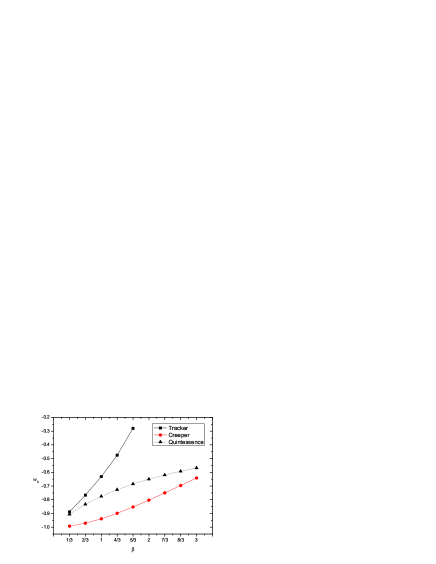
Figure 1: Present value of the barotropic index $w$ for tachyon tracking solutions (squares) and for creeping solutions for $T_{\rm i}=1$ (circles) with inverse power-law potentials $U\propto T^{-\beta}$. For comparison the result for tracking canonical quintessence is also shown (triangles).

III.1 $U=U_{c}T^{-\beta}$

These potentials lead asymptotically to dS for $\beta<2$ and to a dust attractor for $\beta\geq 2$. The first case is the most viable for obvious reasons, and we have verified that for $T_{\rm i}<0.1$ and $T_{\rm i}^{\prime}=0$ the numerical solutions with $\beta<2$ lie on the asymptotically dS attractor, while for $\beta\geq 2$ and the same initial conditions it is not possible to achieve a cosmology compatible with observations (i.e., $x_{0}=1$). For $T_{\rm i}\gtrsim 0.1$, one goes further and further away from the attractor and enters a creeping regime, in the sense that the evolution depends on the choice for $T_{\rm i}$. In Fig. 1 the value of $w_{0}$ is shown for the tracker solution and for a particular creeping solution with $T_{\rm i}=1$. In general, creepers mimic a cosmological constant more closely than trackers, and, in particular, only a creeping solution is available for $\beta\geq 2$. For comparison we also show the equation of state from tracking canonical quintessence models, which for the same $\beta$ is always more negative than that of the tracking tachyons.

These results can be understood by recalling that in the slow-roll approximation there is a mapping between the DBI scalar and the Klein–Gordon one ben02 ; GKMP . The tachyon energy density is $\varrho_{T}=U(T)/\sqrt{1-\dot{T}^{2}}\approx U(T)+U(T)\dot{T}^{2}/2$, and after a field redefinition $\phi\equiv\int\!\sqrt{U(T)}\,dT$ one obtains a canonical action for a scalar $\phi$ with potential $W(\phi)\equiv U[T(\phi)]$. For $U(T)\sim T^{-\beta}$, one has

$$W(\phi)\sim\phi^{-\tilde{\beta}}\quad,\quad\tilde{\beta}=\frac{2\beta}{2-\beta}\,.$$ (17)

Hence the tachyon tracker for $0<\beta<2$ is dual to the tracking quintessence solution $\tilde{\beta}>0$. From Fig. 1, one can see that any dual pair $(\beta,\tilde{\beta})$ corresponds to almost the same index $w_{0}$ — see in particular the pairs $(2/3,1)$ and $(1,2)$.

The attractor evolution of the fluid components is shown in Fig. 2 together with $w(N)$, for the particular case $\beta=1/3$. The behaviours of these quantities for other values of $\beta$ are all similar. Note that the barotropic index is $w\approx-1$ until matter domination, increases up to $w\approx-0.8$ at redshift $z\sim 10^{2}$, and then decreases towards $-1$. This is consistent with the ‘freezing’ behaviour and its limit of applicability as classified by Ref. CL .

For the creeping solutions (not shown here) the index $w$ is very close to $-1$ up to very late times, when it starts deviating to a softer equation of state.

Figure 2: Evolution of the density parameters and equation of state as a function of $N$ for the inverse power-law tachyon model with $\beta=1/3$. Solid line: $\varrho_{\rm m}/x$; dashed line: $\varrho_{\rm r}/x$; dotted line: $\varrho_{T}/x$. The dot-dashed line is the barotropic index $w$.

In this and all other examples, the onset of dark energy lies in the interval $-1<N<0$, that is, for redshift $z<1.7$. Such late domination by dark energy is essential to prevent an excessive suppression of structure formation growth, see e.g. Ref. BJP .

In Fig. 3 the points predicted by the same models in the $w_{0}$–$w^{\prime}_{0}$ plane are shown together with the $1\sigma$ and $2\sigma$ likelihood contour bounds of Ref. WM . These are based on the first-year SNLS data set ast05 and SDSS eis05 , WMAP3 spe06 , and 2dF ver02 ; haw02 experiments. Note that there is a minimum value for $w^{\prime}_{0}$ around $\beta\approx 0.99$; we have checked that its closeness to 1 is an accident of the particular $\Omega_{\rm m,0}$ used.

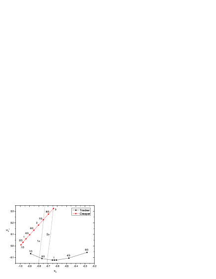
Figure 3: Numerical points in the $w_{0}$-$w^{\prime}_{0}$ plane for tracking solutions (squares) and creeping solutions for $T_{\rm i}=1$ (circles) with inverse power-law potentials $U\propto T^{-\beta}$. The value of $\beta$ is shown at each point, while the dotted lines are the $1\sigma$ and $2\sigma$ likelihood bounds WM . The unlabelled points on the left and right of $\beta=1$ in the tracking curve are $\beta=0.95$ and $\beta=1.05$, respectively.

The conclusion is that there is tracking behaviour for $\beta<2$, and if $T_{\rm i}$ is not too large this operates and gives a well-defined prediction for $w_{0}$, which is however in disagreement with observations unless $\beta$ is quite small. The predicted $w_{0}$ moves closer to $-1$ as the potential flattens, but only once it gets down to about $\beta\lesssim 0.8$ do we start to see compatibility with the $2\sigma$-level bounds. This is even flatter than the equivalent constraint on quintessence, $\beta\lesssim 4/3$. Hence these models are not very pleasant from either a theoretical or experimental point of view. One has to impose $\beta\lesssim 1$ or fine-tune the initial conditions. Relaxing either assumption results in incompatibility with observations. The creeping solution with $T_{\rm i}=1$ (upper curve) gives an example of observationally viable model for $\beta\leq 3$, but at the cost of fine-tuned initial conditions.

One can also make $T^{\prime}_{\rm i}$ big enough that the initial $w$ is close to zero rather than $-1$. Then it dips to $-1$ and increases to join the tracker, eventually giving exactly the same evolution as if one had chosen $T^{\prime}_{\rm i}=0$ at the start. This is exactly the same sequence of epochs that are seen in quintessence models BMR ; if the initial velocity is set high, then the trajectory ‘overshoots’ the tracker, comes to rest at lower potential energy for a while, and eventually rejoins the tracker from below.

We can compare the numerical output for $T_{0}$ with the asymptotic solutions derived in the Appendix, specifically Eq. (33). With $C=0.045$, the ratio $|T_{0}^{\rm num}-T_{0}^{\rm theor}|/T_{0}^{\rm num}$ is always less than 2%. As explained in the Appendix, the asymptotic analytic solution relies on a polynomial rather than monomial potential, and in general they will predict a different variation of $w$. Moreover, the values of $p$ from Eq. (32) are rather small, corresponding to $-2.5\lesssim N_{*}\lesssim-0.5$, where $N_{*}$ is the big bang event; i.e. the asymptotic solution which matches the present evolution has a big bang in the very recent past, and hence can only have become a reasonable approximation very recently. The solution properly approaches the attractor only for large positive $N$, when the contributions of radiation and dust matter are negligible. Nevertheless it appears to give a good estimate of $w_{0}$, though not $w_{0}^{\prime}$.

III.2 $U=U_{c}\exp(1/\mu T)$

This model has a non-zero vacuum energy $U_{c}$ as $T\rightarrow\infty$, which will be achieved asymptotically. It exhibits some features similar to the inverse power-law potential with $\beta<2$, but does not appear to exhibit tracking behaviour. We have fixed $\mu=1$ and checked that this does not result in a loss of generality. For $T_{\rm i}\gtrsim 2$ the solution is very close to de Sitter, $w_{0}\approx-1$ and $0<w^{\prime}_{0}<10^{-3}$, essentially amounting to a creeping solution ($T_{0}\approx T_{\rm i}$) sitting on the asymptotic flat part of the potential.

For smaller $T_{\rm i}\lesssim 1$ the cosmological values today depend on the initial conditions of the model. For $T_{\rm i}=1$ we find $w_{0}\approx-0.95$, $w^{\prime}_{0}\approx 0.04$ and for $T_{\rm i}=0.5$, $w_{0}\approx-0.77$, $w^{\prime}_{0}\approx-0.05$. The solution exits the $2\sigma$ contour at about $T_{\rm i}=0.4$ ($w_{0}\approx-0.70$, $w^{\prime}_{0}\approx-0.14$). One might argue that the initial condition $T_{\rm i}^{\prime}=0$ is inappropriate for this model, since the potential is very steep at small field values. However, we have verified that the slow-roll velocity is small enough to be negligible anyway at least for $T_{\rm i}\geq 0.2$ (which is beyond the observable region). There is no evidence of tracker-type behaviour for $T_{\rm i}\geq 0.2$.

This model does not need fine-tuning of the initial conditions, as the field can lie anywhere on the flat part of the potential. However one has to fix the value of $U_{c}$ by hand in order to reproduce the observed dark energy density, which of course does not resolve the cosmological constant problem.

As in the inverse-power case, we can compare the numerical output of $w_{0}$ with the asymptotic solution Eq. (52), where $\phi_{0}=1/T_{0}^{\rm num}$. When $\phi_{0}\sim 1$ and the approximation giving Eq. (52) breaks down, $|w_{0}^{\rm num}-w_{0}^{\rm theor}|/|w_{0}^{\rm num}|\sim 0.1$, while at large $T_{0}$ one has $|w_{0}^{\rm num}-w_{0}^{\rm theor}|/|w_{0}^{\rm num}|<10^{-3}$ or better. We note that Eq. (53) is negative definite while ${w_{0}^{\rm num}}^{\prime}>0$, and there is disagreement between the two.

III.3 $U=U_{c}\exp(\mu^{2}T^{2})$

This model also has a non-zero vacuum energy $U_{c}$, this time at $T=0$. Fixing $\mu=1$, for $T_{\rm i}<0.1$ one has a de Sitter behaviour ($w_{0}\approx-1$, $0<w^{\prime}_{0}<10^{-3}$), while for increasing $T_{\rm i}$ the barotropic index goes away from $-1$ (for instance, $T_{\rm i}=1$ gives $w_{0}\approx-0.81$, $w_{0}^{\prime}\approx 0.13$).

Checking the numerical output of $w_{0}$ with Eq. (54), where $\phi_{0}=(T_{0}^{{\rm num}})^{2}\ll 1$, one can see that $|w_{0}^{\rm num}-w_{0}^{\rm theor}|/|w_{0}^{\rm num}|<10^{-4}$. Again, Eq. (55) is negative definite while ${w_{0}^{\rm num}}^{\prime}>0$.

Note that lower values of $\mu$ lead even more closely to a cosmological constant behaviour, well inside the $1\sigma$ bound. This may be relevant when trying to construct a model which fits also for inflation, as one needs $\mu^{2}\sim 10^{-8}$ to get the correct level of anisotropies GST .

III.4 $U=U_{c}\exp(-\mu T)$ and $U=U_{c}/\cosh(\mu T)$

When considering the pure exponential potential $U=U_{c}\exp(-\mu T)$, choosing a different starting value of $T$ has no impact on the evolution because a rescaling $T\to T+$ const. simply renormalizes $U_{c}$, which the program then adjusts to give the same present status (corresponding to $w_{0}\approx-0.93$, $w_{0}^{\prime}\approx 0.10$). Therefore we consider directly the hyperbolic cosine potential of Ref. LLM , for which this degeneracy is removed. For $0\lesssim T_{\rm i}\lesssim 0.3$, the solution has $w_{0}\lesssim-0.99$ and $0<w_{0}^{\prime}\lesssim 10^{-2}$, while for larger values of $T_{\rm i}$ the present-day barotropic index becomes larger. We note that the accelerating phase of these solutions is only a transitory epoch before reaching the dust attractor in the future, as shown in Fig. 4 where the equations have been integrated up to positive values of $N$.

Figure 4: Evolution as a function of $N$ of the model $U=U_{c}/\cosh(T)$, in this case extending beyond the present. Solid line: $\varrho_{\rm m}/x$; dashed line: $\varrho_{\rm r}/x$; dotted line: $\varrho_{T}/x$. The dot-dashed and dot-dot-dashed lines are $w$ and $w^{\prime}$, respectively. In this example, the initial condition is $T_{\rm i}=0.5$, for which $w_{0}\approx-0.98$ and $w_{0}^{\prime}\approx 0.03$.

Since one must tune, although not too severely, the initial condition (or, equivalently, $U_{c}$) so as to get viable acceleration today, this and other models leading to a dust regime are not very predictive. They are however capable of explaining the observed dark energy properties.

III.5 $U=U_{c}\exp(-\mu^{2}T^{2})$

This model has a dust attractor whose qualitative features match the previous case. It is not difficult to find suitable initial conditions mimicking a cosmological constant today.

IV Discussion

None of the models we have discussed are very satisfactory. Those which carry reasonable theoretical motivation all end up with a high degree of fine-tuning. Either the potential normalization $U_{c}$ has to be set to match the observed dark energy density, or the initial conditions tuned to the creeping regime, meaning that the present density was already set in place during the early Universe. In either case, this tuning amounts to a restatement of the cosmological constant problem, rather than a resolution. The models which avoid fine-tuning of initial conditions (while still subject to tuning of the normalization), such as the inverse power-law, are constrained by observations into parameter regimes with no theoretical motivation.

The string tachyon with DBI action seems only weakly competitive as a dark energy candidate, and another formulation of the effective theory might have more successful applications. The tachyonic effective action as the lowest-order level truncation of cubic string field theory has been studied only very recently and its cosmological impact has yet to be fully assessed are04 ; AJ ; cut ; AK . An alternative would be to abandon the pure four-dimensional picture (ideally corresponding to a low-energy single or coincident brane configuration in a higher-dimensional spacetime) and consider more general brane–anti-brane setups where open string modes naturally live. However, any modification to Einstein gravity would be severely constrained after nucleosynthesis.

Finally, it was shown that the addition of electric and magnetic fields in the non-BPS brane world volume can slow down the evolution of the inflationary tachyon and relax the fine tuning of the parameters CQS ; cre05 . It might be worth checking whether the insertion of non-trivial fluxes plays some role in the late universe.

Still, the era of high-precision cosmology opened up by microwave background and large-scale structure observations is allowing us to constrain inflationary and dark energy models in a more and more stringent way, selecting some of them from a plethora of possibilities. Here we have given an example of the first stage of such a procedure. The second one will be to develop and refine those models that seem particularly promising, by embedding them in a comprehensive and consistent picture of the cosmological history and its particle theory content.

Appendix A Asymptotic solutions

In this Appendix we derive some analytical asymptotic solutions describing the evolution once the tachyon has become completely dominant.

A.1 Asymptotic solutions for power-law potentials

Inverse power-law potentials, introduced in the context of dark energy in Ref. RP , have no general support from string theory. However, they can be viewed as large-field approximations ($|T|\to+\infty$) of the exact solution fei02

$$a = \exp[p(t/t_{0})^{n}-p]\,,$$ (18)

$$U_{n} = U_{c}\sqrt{1+T^{2n/(n-2)}}\,T^{-4(n-1)/(n-2)}\,,$$ (19)

where we have normalized $a$ so that $a_{0}=1$. We have

$$U_{n} \sim T^{-\beta}=T^{-4(n-1)/(n-2)},$$ (20)

$$n = \frac{2(2-\beta)}{4-\beta}\,,$$ (21)

for $0<n<2$, or

$$U_{n} \sim T^{-\gamma}=T^{-(3n-4)/(n-2)},$$ (22)

$$n = \frac{2(2-\gamma)}{3-\gamma}\,.$$ (23)

for either $n<0$ or $n>2$. The solutions with the potential Eq. (20) are real, nontrivial and expanding if, and only if,

$$N_{*}<0\quad{\rm and}\quad 0<\beta<2\quad(0<n<1)\,,$$ (24)

or

$$N_{*}>0\quad{\rm and}\quad\beta<0\quad(1<n<2)\,,$$ (25)

where $N_{*}\equiv-p$. In the first case, the big bang event is at $N_{*}$ and $N_{*}<N<+\infty$; in the second case, $-\infty<N<N_{*}$. The solutions with the potential Eq. (22) are well behaved when $N_{*}>0$ and either $2<\gamma<3$ ($n<0$) or $\gamma>3$ ($n>2$).

The case given by Eq. (24) is the most interesting since it corresponds to the tracking regime. Using the definition Eq. (21) and neglecting matter and radiation contributions, one has the exact solution

$$x = \left(\frac{N_{*}}{N_{*}-N}\right)^{\beta/(2-\beta)},$$ (26)

$$w = -\frac{x^{\prime}}{3x}-1=(w_{0}+1)\frac{N_{*}}{N_{*}-N}-1\,,$$ (27)

$$w^{\prime} = -\frac{3(2-\beta)}{\beta}(w+1)^{2}\,,$$ (28)

$$T^{\prime 2} = \frac{w+1}{x}$$ (29)

$$= (w_{0}+1)\left(\frac{N_{*}}{N_{*}-N}\right)^{2(1-\beta)/(2-\beta)},$$

$$T = \frac{\beta}{3\sqrt{w_{0}+1}}\left(\frac{N_{*}-N}{N_{*}}\right)^{1/(2-\beta)}+C\,,$$ (30)

where we have assumed $T^{\prime}>0$ ($T>0$), $C$ is an integration constant, and

$$w_{0}+1=-\frac{\beta}{3(2-\beta)}\frac{1}{N_{*}}.$$ (31)

One can find the value of $p$ for the attractor from today’s value of the barotropic index. Inverting Eq. (31),

$$p=\frac{\beta}{3(2-\beta)(w_{0}+1)}.$$ (32)

Also,

$$T_{0} = \frac{\beta}{3\sqrt{w_{0}+1}}+C,$$ (33)

$$T_{0}^{\prime} = \sqrt{w_{0}+1}\,,$$ (34)

$$w^{\prime}_{0} = -\frac{3(2-\beta)}{\beta}(w_{0}+1)^{2}.$$ (35)

The classical stability of these solutions was studied in Refs. AF ; CGST . At late times (i.e., large $T$ and $N$), one has a de Sitter regime for $0<\beta<2$, $\epsilon\to 0$, or an asymptotically dust solution ($\gamma>2$). These solutions are actually attractors. As regards the latter, we note that

$$\dot{T}^{2}=(w_{0}+1)\left(\frac{N_{*}}{N_{*}-N}\right)\to 1,$$ (36)

where we have taken the Carroll limit gib03 (the DBI action then becomes singular) corresponding to tachyon condensation into dust. This expression prescribes a regularization for all the above formulæ, and suggests the following possibility, considered also in Ref. CGST . The only way to balance the increasingly small denominator is to impose that $w_{0}+1\approx 0$; this might mean that if $\gamma>2$, the Universe tends to become dust dominated but only after passing through an accelerating phase. Since the origin of time is arbitrary, such a phase is not positioned unequivocally and it will be determined also by the normalization constant $U_{c}$ of the potential.

A.2 Asymptotic solutions for exponential potentials

In general, a solution for the Friedmann equation in terms of $T$ can be found by noting that, when $w\approx{\rm const}$, the $T$ dependence of the Hubble parameter must be the same as of the tachyon potential, the square root in the denominator of Eq. (9) (with $\varrho=0$) being dimensionless: $x(T)\propto U(T)$. All the exponential potentials we consider can be suitably parametrized so that

$$x=A\exp[(\mu T)^{\alpha}]\,,$$ (37)

where $A=\exp[-(\mu T_{0})^{\alpha}]$ and we have neglected all matter/radiation contributions. Differentiating this equation with respect to $N$ and using the continuity equation ($w^{\prime}=0$), one has

$$3xT^{\prime}=-\alpha\mu^{\alpha}T^{\alpha-1},$$ (38)

which can be integrated from $N$ to today:

$$N=-\frac{3A}{\alpha\mu^{\alpha}}\int_{T_{0}}^{T}dT\,T^{1-\alpha}\exp[(\mu T)^{\alpha}]\,.$$ (39)

Defining the variable $\phi\equiv(\mu T)^{\alpha}$, the integral becomes

$$N = -\frac{3A}{(\alpha\mu)^{2}}\int_{\phi_{0}}^{\phi}d\phi\,\phi^{2(1-\alpha)/\alpha}e^{\phi}$$

$$= -\frac{3A(-1)^{2/\alpha}}{(\alpha\mu)^{2}}\left[\Gamma\left(\frac{2}{\alpha}-1,-\phi\right)-\Gamma\left(\frac{2}{\alpha}-1,-\phi_{0}\right)\right]$$

$$\equiv F(\alpha,\phi)\,,$$ (41)

where $\Gamma$ is the incomplete gamma function. The cases of interest are

$$F(1,\phi) = -\frac{3}{\mu^{2}}(e^{\phi-\phi_{0}}-1)\,,$$ (42)

$$F(-1,\phi) = \frac{3e^{-\phi_{0}}}{\mu^{2}}[\Gamma(-3,-\phi_{0})-\Gamma(-3,-\phi)]\,,$$

$$F(2,\phi) = \frac{3e^{-\phi_{0}}}{(2\mu)^{2}}[\Gamma(0,-\phi)-\Gamma(0,-\phi_{0})].$$ (44)

The first equation implies that

$$T(N)=T_{0}+\frac{1}{\mu}\ln\left(1-\frac{\mu^{2}}{3}N\right)\,.$$ (45)

In order to find $T$ as a function of $N$ in the other cases, Eqs. (LABEL:g-1) and (44) can be expanded around large or small $\phi$: for $\alpha=-1$,

$$\phi\ll 1:\qquad F(-1,\phi) \sim \frac{e^{-\phi_{0}}}{\mu^{2}}\left(\frac{1}{\phi^{3}}-\frac{1}{\phi_{0}^{3}}\right)\,,$$ (46)

$$\phi\gg 1:\qquad F(-1,\phi) \sim \frac{3e^{-\phi_{0}}}{\mu^{2}}\left(\frac{e^{\phi_{0}}}{\phi_{0}^{4}}-\frac{e^{\phi}}{\phi^{4}}\right),$$

while when $\alpha=2$,

$$\phi\ll 1:\quad F(2,\phi) \sim \frac{3e^{-\phi_{0}}}{(2\mu)^{2}}\ln\left(\frac{\phi_{0}}{\phi}\right)\,,$$ (48)

$$\phi\gg 1:\quad F(2,\phi) \sim \frac{3e^{-\phi_{0}}}{(2\mu)^{2}}\left(\frac{e^{\phi_{0}}}{\phi_{0}}-\frac{e^{\phi}}{\phi}\right).$$ (49)

One can then numerically invert the above transcendental functions to get $\phi(N)$ and

$$w = -1-\phi^{\prime}(N)/3\,,$$ (50)

$$w^{\prime} = -\phi^{\prime\prime}(N)/3\,.$$ (51)

When $\phi\ll 1$ (which is the regime typical of the dS-attractor solutions), one can show that

$$w_{0} = \mu^{2}e^{\phi_{0}}\left(\frac{\phi_{0}^{2}}{3}\right)^{2}-1\,,$$ (52)

$$w_{0}^{\prime} = -\frac{4}{3^{3}}\,\mu^{4}e^{2\phi_{0}}\phi_{0}^{7}\,,$$ (53)

for $\alpha=-1$, while

$$w_{0} = \left(\frac{2\mu}{3}\right)^{2}e^{\phi_{0}}\phi_{0}-1\,,$$ (54)

$$w_{0}^{\prime} = -\frac{(2\mu)^{4}}{3^{3}}\,e^{2\phi_{0}}\phi_{0}\,,$$ (55)

for $\alpha=2$. Note that $w^{\prime}$ is always very small in these models.

A.3 Comparison with numerical solutions

Having built the asymptotic analytic solutions, one would like to check whether the numerical behaviour really approaches such solutions at late times. In particular, we want to compare the numerical points in the $w_{0}$–$w_{0}^{\prime}$ plane in parameter space, found via

$$w_{0} = (T^{\prime}_{0})^{2}-1\,,$$ (56)

$$w^{\prime}_{0} = 2w_{0}T^{\prime}_{0}\left[3T^{\prime}_{0}+\frac{(U_{,T})_{0}}{U_{0}}\right]\,,$$ (57)

with the corresponding semi-analytic expressions given by Eqs. (33)–(35) for inverse power-law potentials and by Eqs. (52)–(55) for exponential potentials. The matter content today still amounts to $25\%$ of the total energy density and contributes to the cosmological evolution, so we expect a deviation of the numerical results relative to the asymptotic, pure tachyonic solution.

There is another source of discrepancy one should take into account, namely the approximations implicit in the solutions presented in this Appendix. In the inverse power-law example, while Eqs. (26)–(30) are valid for a polynomial potential as in Eq. (19), the numerical model is actually Eq. (20), and in general the two will give a different running of the barotropic index $w^{\prime}$, Eq. (57). In Sec. III.1 we find that ${w^{\prime}_{0}}^{\rm num}$ and ${w^{\prime}_{0}}^{\rm theor}$ do disagree, but still there is remarkable agreement between $w_{0}^{\rm num}$ and $w_{0}^{\rm theor}$ [the latter comparison is in fact done between $T_{0}^{\rm num}$ and $T_{0}^{\rm theor}(w_{0}^{\rm num})$].

In the case of exponential potentials, the asymptotic models have $w\approx{\rm const.}$ by construction [$x(N)\propto U(N)$] and the equations of motion are much simplified. Again, $w_{0}^{\rm num}\approx w_{0}^{\rm theor}$ to good approximation (see Secs. III.2 and III.3), while a comparison of the running would require a more refined treatment.

References

- (1) C. Armendariz-Picon, V. F. Mukhanov, and P. J. Steinhardt, Phys. Rev. Lett. 85, 4438 (2000) [astro-ph/0004134].
- (2) G. W. Gibbons, Phys. Lett. B 537, 1 (2002) [hep-th/0204008].
- (3) L. P. Chimento, Phys. Rev. D 69, 123517 (2004) [astro-ph/0311613].
- (4) E. J. Copeland, M. Sami, and S. Tsujikawa, hep-th/0603057.
- (5) D. Choudhury, D. Ghoshal, D. P. Jatkar, and S. Panda, Phys. Lett. B 544, 231 (2002) [hep-th/0204204].
- (6) J. Hao and X. Li, Phys. Rev. D 66, 087301 (2002) [hep-th/0209041].
- (7) J. S. Bagla, H. K. Jassal, and T. Padmanabhan, Phys. Rev. D 67, 063504 (2003) [astro-ph/0212198].
- (8) M. R. Garousi, M. Sami, and S. Tsujikawa, Phys. Rev. D 70, 043536 (2004) [hep-th/0402075].
- (9) E. J. Copeland, M. R. Garousi, M. Sami, and S. Tsujikawa, Phys. Rev. D 71, 043003 (2005) [hep-th/0411192].
- (10) V. H. Cardenas, Phys. Rev. D 73, 103512 (2006) [gr-qc/0603013].
- (11) G. Shiu and I. Wasserman, Phys. Lett. B 541, 6 (2002) [hep-th/0205003].
- (12) T. Padmanabhan and T. R. Choudhury, Phys. Rev. D 66, 081301 (2002) [hep-th/0205055].
- (13) Y. Wang and P. Mukherjee, astro-ph/0604051.
- (14) H. B. Benaoum, hep-th/0205140.
- (15) V. Gorini, A. Kamenshchik, U. Moschella, and V. Pasquier, Phys. Rev. D 69, 123512 (2004) [hep-th/0311111].
- (16) D. N. Spergel et al., astro-ph/0603449.
- (17) M. Fairbairn and M. H. G. Tytgat, Phys. Lett. B 546, 1 (2002) [hep-th/0204070].
- (18) P. J. Steinhardt, L. M. Wang, and I. Zlatev, Phys. Rev. D 59, 123504 (1999) [astro-ph/9812313].
- (19) L. M. Wang, R. R. Caldwell, J. P. Ostriker, and P. J. Steinhardt, Astrophys. J. 530, 17 (2000) [astro-ph/9901388].
- (20) R. R. Caldwell and E. V. Linder, Phys. Rev. Lett. 95, 141301 (2005) [astro-ph/0505494].
- (21) E. V. Linder, Phys. Rev. D 73, 063010 (2006) [astro-ph/0601052].
- (22) A. Frolov, L. Kofman, and A. Starobinsky, Phys. Lett. B 545, 8 (2002) [hep-th/0204187].
- (23) L. R. W. Abramo and F. Finelli, Phys. Lett. B 575, 165 (2003) [astro-ph/0307208].
- (24) T. Padmanabhan, Phys. Rev. D 66, 021301 (2002) [hep-th/0204150].
- (25) J. M. Aguirregabiria and R. Lazkoz, Phys. Rev. D 69, 123502 (2004) [hep-th/0402190].
- (26) I. Zlatev, L. M. Wang, and P. J. Steinhardt, Phys. Rev. Lett. 82, 896 (1999) [astro-ph/9807002].
- (27) S. Kachru, R. Kallosh, A. Linde, and S. P. Trivedi, Phys. Rev. D 68, 046005 (2003).
- (28) N. Lambert, H. Liu, and J. Maldacena, hep-th/0303139.
- (29) P. Astier et al., Astron. Astrophys. 447, 31 (2006) [astro-ph/0510447].
- (30) D. J. Eisenstein et al., Astrophys. J. 633, 560 (2005) [astro-ph/0501171].
- (31) L. Verde et al., Mon. Not. R. Astron. Soc. 335, 432 (2002) [astro-ph/0112161].
- (32) E. Hawkins et al., Mon. Not. R. Astron. Soc. 346, 78 (2003) [astro-ph/0212375].
- (33) P. Brax, J. Martin, and A. Riazuelo, Phys. Rev. D 62, 103505 (2000) [astro-ph/0005428].
- (34) I. Ya. Aref’eva, AIP Conf. Proc. 826, 301 (2006) [astro-ph/0410443].
- (35) I. Ya. Aref’eva and L. V. Joukovskaya, J. High Energy Phys. 10, 087 (2005) [hep-th/0504200].
- (36) G. Calcagni, J. High Energy Phys. 05 (2006) 012 [hep-th/0512259].
- (37) I. Ya. Aref’eva and A. S. Koshelev, hep-th/0605085.
- (38) D. Cremades, F. Quevedo, and A. Sinha, J. High Energy Phys. 10 (2005) 106 [hep-th/0505252].
- (39) D. Cremades, Fortsch. Phys. 54, 357 (2006) [hep-th/0512294].
- (40) B. Ratra and P. J. E. Peebles, Phys. Rev. D 37, 3406 (1988).
- (41) A. Feinstein, Phys. Rev. D 66, 063511 (2002) [hep-th/0204140].
- (42) G. W. Gibbons, Class. Quantum Grav. 20, S321 (2003) [hep-th/0301117].