The X-ray Properties of Optically-Selected Galaxy Clusters

Abstract

We stacked the X-ray data from the ROSAT All Sky Survey for over 4,000 clusters selected from the 2MASS catalog and divided into five richness classes. We detected excess X-ray emission over background at the center of the stacked images in all five richness bins. The interrelationships between the mass, X-ray temperature and X-ray luminosity of the stacked clusters agree well with those derived from catalogs of X-ray clusters. Poisson variance in the number of galaxies occupying halos of a given mass leads to significant differences between the average richness at fixed mass and the average mass at fixed richness that we can model relatively easily using a simple model of the halo occupation distribution. These statistical effects probably explain recent results in which optically-selected clusters lie on the same X-ray luminosity-temperature relations as local clusters but have lower optical richnesses than observed for local clusters with the same X-ray properties. When we further binned the clusters by redshift, we did not find significant redshift-dependent biases in the sense that the X-ray luminosities for massive clusters of fixed optical richness show little dependence on redshift beyond that expected from the effects of Poisson fluctuations. Our results demonstrate that stacking of RASS data from optically selected clusters can be a powerful test for biases in cluster selection algorithms.

1 Introduction

The primary objective of many new extragalactic surveys is to determine the equation of state of the dark energy. One approach is to determine the evolution of the cluster mass function with redshift, which depends on dark energy through the growth factor and the volume element (e.g., Haiman, Mohr & Holder 2001; Huterer & Turner 2001; Podariu & Ratra 2001; Kneissl et al. 2001; Newman et al. 2002; Levine, Schulz, & White 2002; Majumdar & Mohr 2003; Hu 2003). Clusters are identified using some observable proxy for their mass over a broad range of redshifts and the proxy must then be calibrated to compare the results to the theoretically predicted mass functions. Possible proxies and identification methods are the optical richness of the cluster (e.g., Abell 1958; Huchra & Geller 1982; Dalton et al. 1992; Postman et al. 1996, 2002; Zaritsky et al. 1997; Gonzalez et al. 2001; Bahcall et al. 2003; Gal et al. 2003; Gladders & Yee 2005), the X-ray luminosity or temperature (e.g., Gioia et al. 1990; Henry et al. 1992; Rosati et al. 1995,1998; Ebeling et al. 1998, 2000; Böhringer et al. 2000, 2004; Bauer et al. 2002; Giacconi et al. 2002), the Sunyaev-Zeldovich decrement (e.g., Carlstrom et al. 2000; LaRoque et al. 2003) and the weak lensing shear (e.g., Wittman et al. 2001; Dahle et al. 2002; Schirmer et al. 2003). Examples of large scale surveys planning on using these methods are the Dark Energy Survey (DES using optical richness, Sunyaev-Zeldovich and weak lensing), the Large Synoptic Survey Telescope (LSST optical richness and weak lensing) and the Supernova / Acceleration Probe (SNAP optical richness and weak lensing). This is in addition to smaller scale surveys based on optical richness such as the SDSS cluster surveys (Goto et al. 2002; Bahcall et al. 2003) and the Red Cluster Sequence Survey (RCS, Gladders & Yee 2005).

A persistent worry about optically selected cluster samples is that chance projections of foreground and background galaxies significantly bias the resulting catalogs. The problem can range from false positives, detections of non-existent clusters, to a richness bias in which chance projections lead to overestimates of the cluster richness. The problems should be more severe for higher redshift and lower richness clusters because the effects of a chance projection increase as the number of detectable galaxies in the cluster diminishes. One approach to checking the extent to which a cluster finding algorithm is affected by these issues is to generate mock galaxy catalogs matching the actual data as closely as possible, find clusters in the mock catalogs and then compare the output and input catalogs (e.g., Kochanek et al. 2003; Miller et al. 2005). In general these comparisons have found only modest biases. A second approach is to compare the mass estimates based on the optical richness to those from another method. At present this has meant examining either the X-ray properties (e.g., Bahcall 1977; Donahue et al. 2002; Kochanek et al. 2003; Popesso et al. 2004) or the weak lensing masses (e.g., SDSS/RCS) of the optically-selected clusters.

A basic problem of most existing tests of optically-selected cluster catalogs using X-ray data is that the comparisons are made to catalogs of X-ray clusters rather than through X-ray observations of the optically-selected clusters. While this provides a simple means of calibrating the relationship between optical and X-ray properties, it is not an optimal approach to searching for biases in the optical selection methods. The problems could be more severe because several recent studies (e.g., Bower et al. 1997; Lubin, Mulchaey & Postman 2004; Gilbank et al. 2004) have found offsets between the X-ray temperature-optical richness relations of local and higher redshift optically-selected clusters even though the clusters lie on the same X-ray temperature-luminosity relations.

In this paper we address these questions by measuring the mean X-ray properties of a sample of galaxy clusters selected from the 2MASS survey (Kochanek et al. 2003, 2006 in preparation) by averaging (“stacking”) the ROSAT All-Sky Survey (RASS, Voges et al. 1999) data for the clusters as a function of richness and redshift. We outline the cluster catalog and our procedures for analyzing the RASS data in §2. In §3 we discuss the theoretical differences between measuring the mean properties of clusters at fixed richness rather than fixed mass. In §4 we present our results for the correlations between the optical richness, X-ray properties and cluster mass estimates, as well as the dependence of the results on cluster redshift. We summarize our results in §5. We assume that $H_{0}=70~{}\rm{km~{}s^{-1}~{}Mpc^{-1}}$, $\Omega_{\rm m}=0.3$, and $\Omega_{\Lambda}=0.7$ throughout the paper.

Figure 1: RASS images of four clusters over-plotted with probable cluster members (squares, $>50\%$ likelihood of membership as determined from the cluster finding algorithm in Kochanek et al. 2003) and field galaxies (X symbols, $<50\%$ likelihood) along with the error ellipse for the cluster centroids provided by optical cluster detection algorithm. Panel A shows the typical cluster, where the optical position is roughly consistent with the X-ray position. Panel B shows an example where the existence of a cluster is correctly inferred in the optical catalog, but the position is seriously in error. Panels C and D show two examples where the optical cluster is confused by the presence of multiple (or merging) clusters.

Figure 2: The stacked ROSAT images of 2MASS clusters in richness bins 0–4 and at random positions. The images are 2.0, 2.0, 1.5, 1.0, 1.0, and 1.0 $h_{70}^{-1}$Mpc in radius for richness bins 0–4 and the random positions. The contours are drawn at levels of 1–4 $\sigma$ above the background. Excess X-ray emission is clearly detected in all richness bins, whereas the stacked image using random positions does not show any significant emission at the center.

2 The Cluster Catalog and The X-ray Data

The cluster catalog we use was selected from the 2MASS infrared survey (Skrutskie et al. 2006) using the matched filter algorithm of Kochanek et al. (2003) applied to the 380,000 galaxies with K$\leq 13.25$ mag (2MASS 20 mag/arcsec² circular, isophotal magnitudes) and Galactic latitude $|b|>5^{\circ}$. For the purposes of this paper we are interested only in the richness $N_{*666}$ and the redshift $z$ of the cluster. The richness $N_{*666}$ is defined to be the number of $L>L_{*}$ galaxies inside the (spherical) radius $r_{*666}$ where the galaxy over density is $\Delta_{N}=200\Omega_{M}^{-1}\simeq 666$ times the mean density based on the galaxy luminosity function of Kochanek et al. (2001). This radius would match the radius with a mass over density of $\Delta_{M}=200$ for $\Omega_{M}=0.3$ and a bias factor of unity. Clusters were included in the final catalog if they had likelihoods $\ln L\geq 10$ and if the cluster redshift was below that at which the cluster would contain one galaxy inside $r_{*666}$ at the magnitude limit of the survey. These selection limits were determined by examining how cluster likelihoods changed as a function of the limiting magnitude of the input galaxy catalog. We divided the cluster catalog into five richness bins, $N_{*666}\geq 10$, $10>N_{*666}\geq 3$, $3>N_{*666}\geq 1$ and $1>N_{*666}\geq 0.3$, which we will refer to as richness bins 0 (richest) to 4 (poorest) respectively. There are 191, 862, 1283, 1298 and 699 clusters in the bins. We matched our cluster catalog to the Abell cluster catalog and found most matches are from our richness bins 0, 1, and 2.

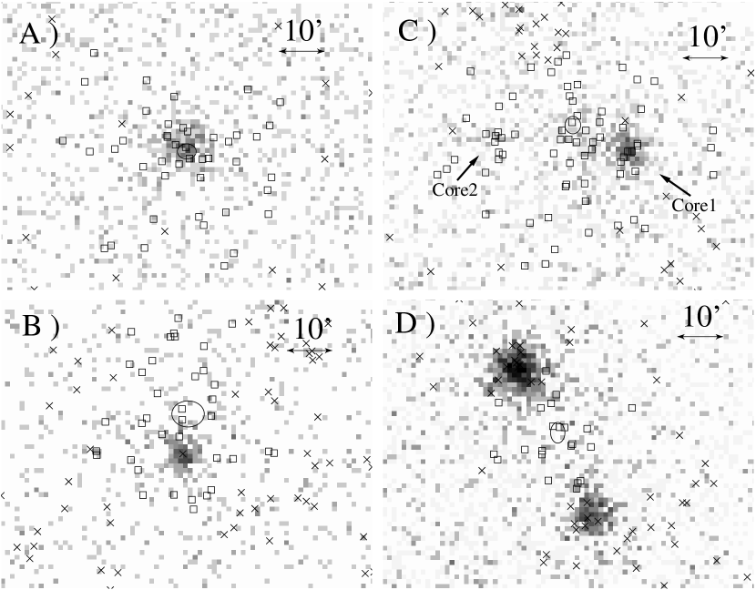
We use the RASS to determine the average properties of the optically-selected clusters, since it is the only recent X-ray survey with the necessary sky coverage. Pointed observations with ROSAT, Chandra, or XMM-Newton are not useful because they would include only a small fraction of the objects in our catalog and represent a biased sampling of the catalog. The RASS data are fairly uniform in both integration time and the average point spread function because the data were obtained by scanning the satellite over the sky. The RASS data and the exposure maps, arranged in $6.4\times 6.4$ square degree fields, were obtained through the High Energy Astrophysics Science Archive Research Center (HEASARC). We extracted the X-ray data in fixed physical regions around the clusters of 2.0, 2.0, 1.5, 1.0, and 1.0 $h_{70}^{-1}$Mpc radius for richness bins 0–4. These scales were chosen to be large enough to estimate the mean X-ray backgrounds since the background must be subtracted for our analyses of the X-ray images and spectra. We ignored the 17% of the clusters for which the extraction regions extended outside the edges of the standard RASS images. The typical exposure time for each cluster is $\sim 400$ sec, and we dropped the $\sim 1\%$ of clusters with exposure times exceeding $1500$ sec (mostly near the poles of the RASS survey) so that they would not dominate the signal-to-noise ratio of the average. Since we are testing the optical catalog, dropping clusters because of the characteristics of the X-ray survey should have no consequences for our results. We did not distinguish between the different observing stripes of the RASS, which have different observing times and backgrounds, instead simply using the average exposure time and background of the combined data. These differences were usually small (less than 10%) and should have little effect on our analysis. Some examples of the optical and X-ray clusters are shown in Figure 1.

We must also remove contaminating sources from each cluster field. We removed the bright point sources in the RASS bright source catalog (Voges et al. 1999) and replaced them with the average of the regions surrounding them (annuli with inner and out radii of 1.5 and 2.5 times the extent of the point sources). As for the bright extended sources detected in the RASS bright source catalog, in most cases they are the clusters we need to stack, although we identified and excluded two clusters with emission from supernova remnants in our extraction region. Finally, approximately 4% of the clusters had additional optical clusters in the extraction annulus. In these cases, we only analyzed the richest cluster. In the cases (five in total) where two clusters are of comparable richness, we excluded both of them as the optical positions tend to be poorly estimated, and sometimes, the optical detection algorithm only found one cluster, locating the optical centroid between the two X-ray clusters. One such example is shown in Figure 1d. After applying all these filters, we were left with 157, 670, 1004, 1057, and 497 clusters for richness bins 0–4, respectively.

Figure 3: The stacked X-ray surface brightness profiles as a function of richness and for random positions. All clusters were background subtracted and normalized to a common distance of 100 Mpc and by their $N_{*666}$ values. The dashed lines indicate the level of the subtracted background and the dash-dotted lines are the best fit $\beta$ models for each bin.

Figure 4: Histogram of offsets between optical and X-ray centroids.

Figure 5: The stacked ROSAT spectra of clusters in richness bins 0–4 and their best fit thermal plasma models.

2.1 Surface Brightness Profiles

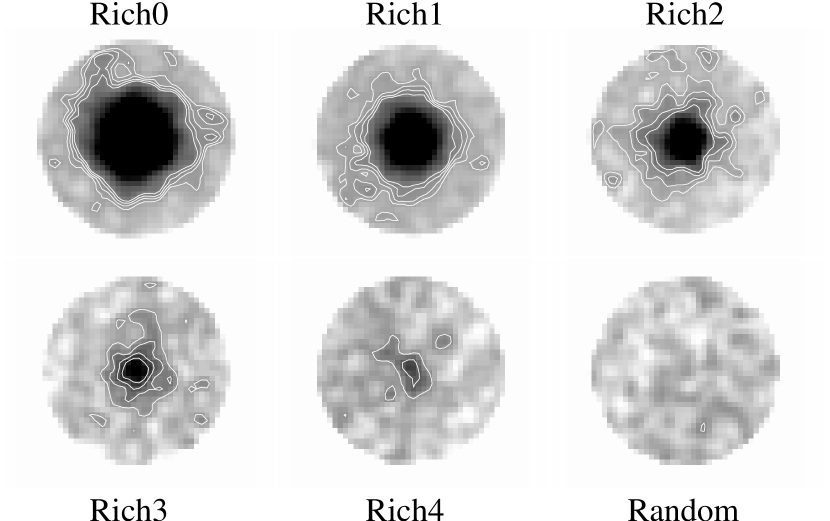
We produce the stacked images by rescaling the data for each cluster to a common distance of 100 Mpc. In addition to adjusting the photon positions, we weight each photon by the square of the ratio between the cluster distance and 100 Mpc. We binned the X-ray images with pixel sizes of 100, 100, 75, 50, and 50 $h_{70}^{-1}$kpc for richness bins 0–4 and then smoothed them with a Gaussian with a dispersion of one pixel. We clearly detect X-ray emission from the clusters in all five richness bins, as shown in Figure 2. The significance contours in Figure 2 apply to the individual pixels, so the sources as a whole are detected at much higher confidence levels than indicated by the contours. For example, although the peak of the emission from the poorest richness bin is only $2\sigma$ above the background, the emission as a whole is detected at about $7\sigma$. We also used bootstrap re-sampling to test the significance of the X-ray emission of the poorest richness bin. First, we tested whether the emission was dominated by a small subset of the objects by randomly drawing identically sized samples from the original sample with replacement and then analyzing the simulated sample. In each of the 100 trials there was excess X-ray emission detected at over 3$\sigma$, and in 94 out of 100 trials the cluster was detected at over 5$\sigma$. If, on the other hand, we stack data from an equal number of random positions with $|b|>5^{\circ}$ and excluding our standard regions near the 2MASS cluster positions, only 8 out of 100 trials have 3$\sigma$ detections and no trials are detected at over 4$\sigma$. One such image is shown in Figure 2. Based on these simulations, we estimate that we detect the richness 4 clusters at greater than the 99% confidence level. In the outer, background regions of the images, the different richness bins have consistent background flux levels and when azimuthally smoothed they show the flat profile expected for convergence.

The background-subtracted surface brightness profiles for each richness bin are shown in Figure 3, where we have used radial bins of constant area, normalized the surface brightness profile by the optical richness $N_{*666}$ and scaled the results to a luminosity distance of 100 Mpc. We subtracted the background for each cluster before we rescaled the data. Like the stacked images, the surface brightness profiles clearly show excess emission above the background for all richness bins, while the profile from stacking random positions does not. We fit the profiles with a standard $\beta$ model, $S(R)=S_{0}(1+R^{2}/R_{c}^{2})^{-3\beta+1/2}$ obtaining the results presented in Table 1. We obtain similar results whether we fit the background-subtracted profiles directly or include an additional parameter to fit any residual background level. When we include an additional parameter for the residual background, its value is found to be consistent with zero. Our estimates of the slope $\beta$ are consistent with typical values for clusters (e.g., Xu et al. 2001; Sanderson et al. 2003), even consistent with the trend of decreasing $\beta$ with decreasing cluster temperature (e.g., Horner et al. 1999; Sanderson et al. 2003) for richnesses 0–3. The $\beta$ values obtained for the two poorest richness bins have large uncertainties. We do, however, find larger core sizes than studies of individual clusters (e.g., Neumann & Arnaud 1999; Xu et al. 2001; Sanderson et al. 2003; Osmond & Ponman 2004), ranging from roughly twice as large for richness bin 0 to more than 5 times as large for richness bin 4, although the estimates for the poorest richness bins are very uncertain. This is not due to the RASS PSF, which is equivalent to a source size of $\sim 20$ kpc at a typical cluster redshift of $z\sim 0.04$. Part of the problem must be a smearing of the X-ray cores by errors in the estimates of the optical centroids. We matched our stacked clusters with the ROSAT extended source catalog and plotted the histogram of offsets between optical and X-ray centroids in Figure 4. The median offset of 0.14 Mpc is consistent with the large core sizes obtained for our stacked images in richness bins 0 and 1 compared with those obtained from individual clusters. The distribution of offsets is very similar to other studies (e.g., Adami et al. 1998; Lopes et al. 2006) when comparing optically-selected clusters and ROSAT clusters. Some of the large offsets are caused by merging clusters where the X-ray image has two cores and the optical centroid is set in between of the X-ray cores (e.g., Figure 1b), and in some other cases the large offset could be due to various other problems (e.g., Figure 1c). We also show one case where the optical centroid matches excellently with the X-ray centroid in Figure 1a. Although we obtain larger cores in our stacked images, the average X-ray properties of the clusters should be little affected.

2.2 Cluster Luminosities, Temperatures and Entropies

In order to estimate the luminosities and temperatures we need to model the X-ray spectra of the clusters. We started by eliminating the 13% of clusters with Galactic absorption column densities higher than $10^{21}$cm^-2. We analyzed the spectra using XSPEC (Arnaud 1996) using the rmf file for the PSPCC detector available from HEASARC. Although the RASS contains some PSPCB observations, they are a small minority of the observations and the rmf files for the two detectors are very similar. Because the RASS was carried out by scanning the sky, there is one additional complication arising from the corrections for vignetting and the off-axis telescope response. We can use two possible calibration files for our analyses. The first approach is to use the standard rsp file provided in the calibration package (which is equivalent to the on-axis arf+rmf files) combined with the vignetting-corrected exposure map. This approach will bias the spectral fits because the true vignetting correction is energy-dependent. The second approach is to use the off-axis arf file. This will lead to unbiased spectral fits, but the RASS images have already corrected the exposure times for the effects of vignetting, so we will be double-counting this correction when we use the off-axis arf file. Fortunately, this simply leads to a normalization offset in the 0.1–2.4 keV flux of a constant factor of $1.44$ that we can determine from the flux differences between the two approaches. We adopt this latter approach with the correction to the fluxes. We generated the off-axis arf files using the pcarf software tool from the XSELECT and FTOOLS packages. We extracted the spectra of the stacked clusters out to radii of 1.5, 1.5, 0.9, 0.65, and 0.4 Mpc for richness bins 0–4, respectively. For each cluster we subtracted the background and normalized the data to the mean redshift of the stacked clusters ($z=0.0816$, 0.0678, 0.0539, 0.0387, and 0.0273 for richness bins 0–4) and then averaged the arf files based on the weighted number of photons in each cluster. Averaging of arf files has little effect on the results because they are all fairly similar due to the nature of the RASS observations.

We fit the spectra with a thermal plasma model (Raymond & Smith 1977) modified by the mean Galactic absorption. We were unable to determine the metallicity from the data, so we assumed a metallicity of $1/3$ solar (e.g., Baumgartner et al. 2005). The redshift was set to the mean redshift of the clusters in each richness bin. We did not worry about the small spread in the true K-corrections for the spectra across each bin because the low redshift of the sample (see Table 1) makes this a small effect. The spectra and their best fit models are shown in Figure 5 and the fitting results are presented in Table 2. We obtained acceptable fits for all richness bins, indicating that the emission is consistent with that from hot gas for all richness bins. As expected, the temperature decreases from rich to poor clusters, and the soft X-ray sensitivity of ROSAT (0.1–2.4 keV) allows us to measure the temperature of the poor clusters more accurately than for rich clusters. Given the temperatures, we can also estimate the bolometric X-ray luminosity. Table 2 presents the estimate for the luminosity within $R_{*666}$ found by using the $\beta$ model fits from §2.1 to correct from the spectral extraction aperture to $R_{*666}$. These corrections were quite small, amounting to multiplicative factors of only 1.06, 0.92, 1.01, 0.99, and 1.03 for richness bins 0–4, respectively. In addition to the error estimates provided by the spectral fits, we also estimated the uncertainties by bootstrap re-sampling the data. For each richness bin we generated 500 random samples by drawing the same number of clusters from those in each richness bin with replacement. These bootstrap estimates of the uncertainties should represent systematic uncertainties better than the purely Poisson uncertainties of the standard fits. In general, the bootstrap uncertainties are slightly larger than the standard errors found from the spectral fits, but usually not by large margins.

While the best fit Galactic ${N}_{\rm H}$ values are consistent with our ${N}_{\rm H}$ cut of $10^{21}$cm^-2, there is a worrisome correlation of ${N}_{\rm H}$ with richness. The estimate of the Galactic absorption is dominated by the lowest energy bins. We ran several fits with fixed ${N}_{\rm H}$ values in the range spanned by the results of Table 2, finding that the overall fits become worse for the richness bins best fit by a different value for ${N}_{\rm H}$, but that the luminosity and temperature estimates change little compared to the statistical errors of the original estimates. We found that we could not analyze the high Galactic absorption clusters at all because of strong degeneracies between the estimates of the temperature and the absorption. Potentially, the origin of the problem could be the presence of an additional soft emission component in the low richness clusters, but we will not investigate this possibility here because it has no effect on our general results and is an area of considerable controversy (e.g., Bregman & Lloyd-Davies 2006).

We also estimated the mean gas entropy, $S=T/n_{e}^{2/3}$, as a direct test of the thermodynamic state of the clusters and the effects of heat transport or energy injection (e.g., Ponman, Cannon, & Navarro 1999; Lloyd-Davies, Ponman, & Cannon 2000; Ponman et al. 2003). We estimated the electron number density $n_{e}$ from the surface brightness profiles derived in §2.1 and the temperature from the spectral fits. We assumed a constant temperature with radius. As we discussed in §2.1, we systematically obtain larger core radii than analyses of individual clusters, and an underestimate of the central surface brightness will lead to an overestimate of the central entropy. Therefore, we focus on the entropy on scales of $0.5r_{*666}$ where we should be insensitive to this problem.

We further divided the each of the first four original bins into two narrower bins. We followed the same procedure described in this section to obtain their temperatures and the bolometric X-ray luminosities (Table 2).

2.3 Cluster Masses

Finally, we estimated the mean cluster masses inside $r_{*666}$ assuming hydrostatic equilibrium,

$$M_{grav}(<r)=-\frac{kT(r)r}{G\mu m_{p}}\left(\frac{d\ln{\rho(r)}}{d\ln{r}}+\frac{d\ln{T(r)}}{d\ln{r}}\right),$$ (1)

using our $\beta$-models from §2.1, $\mu=0.61$ (Arnaud 2005a), and assuming an isothermal temperature profile. This is not a trivial exercise given the stacked data. First, we cannot accurately measure the mass profile in the inner regions of the clusters where we can accurately measure the temperature because of the smearing created by the position uncertainties discussed in §2.1. Second, we cannot accurately measure the temperature in the outer regions, or equivalently, the slope of the temperature profile, because we have insufficient counts in the outer regions. We expect the first issue is less severe since the mass obtained by this method mainly depends on the temperature and its gradient at a sufficiently large radius, which is less affected by the profile of the inner slope. The isothermal assumption will possibly lead to an over estimate of mass by $\sim$15% (Sanderson et al. 2003). These uncertainties are smaller than those introduced from cluster temperature measurements for most cases. We estimated $r_{200}$ and $M_{200}$ from the mass profiles by calculating the mass and radius where the mass over density is 200 times the critical density. We also performed the same analysis to the narrower richness bins. Again, we expect the dominant uncertainties for masses are from the cluster temperatures.

There are offsets between the $M_{*666}$ and $M_{200}$ mass estimates that simply reflect the differences between $r_{*666}$ and $r_{200}$. The two radii are not simply proportional to each other, as illustrated in Fig. 6. The difficulty probably arises because $r_{*666}$ is computed from the fitted richness and a fixed three dimensional galaxy distribution because it is not possible to determine the galaxy distribution for the individual clusters with any accuracy (see Kochanek et al. 2003). To investigate this further we need to examine the optical properties of the stacked clusters, which will be the subject of a later study (Morgan et al. 2007 in preparation). Our estimate of $r_{200}$ from the stacked X-ray images is consistent with scaling relations from the measured temperatures, as illustrated by the values of $r_{180}$ derived from the temperature and the temperature-radius scaling relation from Evrard et al. (1996). Note, however, that the shifts in the masses due to the different radii are too small to affect the overall structure of the mass-temperature-richness correlations.

3 Averaging Cluster Properties at Fixed Optical Richness

Before discussing the results from measuring the mean luminosity, temperature or mass as a function of optical richness, it is necessary to discuss the important distinction between averaging at fixed richness and averaging at fixed mass (see Berlind & Weinberg 2002). For simplicity, we will assume a simple model for the halo mass function,

$$n_{M}(M)={dn\over dM}\propto M^{-x}\exp\left(-(M/M_{1})^{y}\right)$$ (2)

with $x\simeq 1.88$ and $\log(M_{1}/M_{\odot})\simeq 14.6$ and $y\simeq 0.73$ closely reproducing a concordance cosmology mass function at $z=0$. Since only higher mass halos form groups and clusters of massive galaxies (our cluster finder is not designed to find galaxies with halos of lower luminosity satellites), we must truncate the halo mass function $n_{M}(M)$ at some point for it to model the cluster mass function $n_{c}(M)$. We model this by using $n_{c}(M)=n_{M}(M)$ for $M>M_{0}$ and then truncating it at lower masses

$$n_{c}(M)=n_{M}(M_{0})\exp\left(-{\log^{2}\left(M/M_{0}\right)\over 2\Delta^{2}}\right)\quad\hbox{for}\quad M<M_{0}$$ (3)

over a logarithmic mass range $\Delta$. On average, a cluster of mass $M$ contains

$$\langle n\rangle=N_{1}\left({M\over M_{1}}\right)^{\gamma}{\Gamma[1+\alpha,L(z)/L_{*}]\over\Gamma[1+\alpha,1]}=N_{1}\left({M\over M_{1}}\right)^{\gamma}c(z)$$ (4)

observable galaxies, where $N_{1}$ is the number of $L>L_{*}$ galaxies for a cluster of mass $M_{1}$ and the ratio of Gamma functions $c(z)$ corrects from the number of $L>L_{*}$ galaxies to the number of galaxies down to the luminosity $L(z)$ corresponding to the flux limit of the galaxy survey at the cluster redshift $z$. The galaxy luminosity function is modeled as a Schechter function with slope $\alpha=-1.09$ and break luminosity $M_{K*}=-24.16$ mag assumed by the cluster finder based on the Kochanek et al. (2003) K-band luminosity functions and with a limiting magnitude of $K_{lim}=13.25$ mag. A particular cluster, however, will contain $n$ galaxies drawn from the conditional probability function for a cluster of mass $M$ having $n$ galaxies,

$$P(n|M)={\langle n\rangle^{n}\over n!}\exp(-\langle n\rangle)$$ (5)

which we assume to be the Poisson distribution. In general, the cluster catalogs are roughly complete to the limit of $n\geq 3$ inside the radius of the filter (see White & Kochanek 2002; Kochanek et al. 2003), and this turns out to be the best fit estimate of the selection limit when we apply the Poisson model to the data. The richness estimate assigned to the cluster is not the observed number of galaxies $n$, but the estimated number of $L>L_{*}$ galaxies, $N_{*}=n/c(z)$. For our analytic models, we will further assume that there are perfect correlations $T(M)$ and $L_{X}(M)$ between the X-ray properties and the mass. The combination of these assumptions is essentially a simple example of a halo occupation distribution (HOD) model (e.g. Yang et al. 2005, Zheng et al. 2005) for the clusters.

When we stack the X-ray data for cluster of fixed observed richness, $N_{*}$, we compute mean values of the form, given here for the mean mass,

$$\langle M(N_{*},z)\rangle={\int_{0}^{\infty}dMMn_{c}(M)P(N_{*}c(z)|M)\over\int_{0}^{\infty}dMn_{c}(M)P(N_{*}c(z)|M)}.$$ (6)

If we set $\gamma=1$, so that the number of galaxies is proportional to the mass, and use a sharp cutoff $\Delta=0$ in the cluster mass function, then the integrals can be done analytically to find that

$$\langle M(N_{*},z)\rangle={M_{1}\over 1+N_{1}c(z)}{\Gamma[2-x+N_{*}c(z),{M_{0}\over M_{1}}(1+N_{1}c(z))]\over\Gamma[1-x+N_{*}c(z),{M_{0}\over M_{1}}(1+N_{1}c(z))]}$$ (7)

where $\Gamma[a,b]$ is an incomplete Gamma function. If we had averaged at fixed mass, we would simply find that the mean mass is $M(N_{*})=M_{1}(N_{*}/N_{1})$, and it is interesting to examine how the average at fixed richness differs from that at fixed mass. If we consider rich clusters with many galaxies ($M\gg M_{0}$, $N_{*}c(z)\gg 1$) then we find that

$${\langle M(N_{*},z)\rangle\over M(N_{*})}=\left[1+{1-x\over N_{*}c(z)}\right]\left[1+{1\over N_{1}c(z)}\right]^{-1}.$$ (8)

The Poisson fluctuations bias the average mass at fixed richness to be low, with a fractional amplitude of order the number of detectable galaxies in the cluster. This is essentially a Malmquist bias due to the steep mass function – more low mass clusters Poisson fluctuate up to the fixed richness than high mass clusters fluctuate down to it. The more interesting limit is that of very low richness clusters. Very low richness clusters will always be close to the cluster detection limit, so let us set $N_{*}c(z)=3$ and take the limit of very low richness ($N_{*}\rightarrow 0$) to find that

$$\langle M(N_{*},z)\rangle\rightarrow M_{0}.$$ (9)

The only way to get an apparently very low richness cluster is as a Poisson fluctuation of a cluster with $M\simeq M_{0}$, so the mean mass converges to $M_{0}$. Thus, compared to averaging properties of clusters at fixed mass, clusters averaged at fixed luminosity should be biased lower in mass for rich clusters and higher in mass for poor clusters even before considering any selection effects. As we shall see, this simple model explains all the results that follow.

Figure 6: The relationship between cluster scaling radius and optical richness $N_{*666}$. The filled circles are $r_{*666}$ obtained from optical algorithm, the squares are $r_{180}$ converted from mean temperature (Evrard et al. 1996), and the X symbols are $r_{200}$ calculated from our mass profile for stacked clusters. The radius $r_{*666}$ is algebraically related to $N_{*666}$ because of the fixed model for the spatial distribution of the galaxies (see Kochanek et al. 2003).

Figure 7: The relationship of the bolometric X-ray luminosity to the temperature. The open and filled circles are the results from our stacking the clusters as a function of richness, and the solid line is the best fit Poisson model (see §3) to these results. The filled circles are for the five standard richness bins, while the open circles are the results found for the narrower bins obtained by dividing the first four richness bins in half. The open triangles are the results found for the middle redshift bin (see Figs. 13, 14) when we divide the clusters in redshift sub-bins. The error bars on the circles are the bootstrap estimates of the errors. The squares show the results for individual 2MASS clusters drawn from the literature. The dashed, dotted, dash-dotted, and dash-dot-dot-dotted lines are from the $L_{X}$–$T_{X}$ relations from Wu et al. (1999), Helsdon & Ponman (2000), and Xue & Wu (2000), and Rosati et al. (2002).

Figure 8: The relationship between mass $M$ and temperature $T$, using the subdivided bins for the first four richness bins. The filled circles are the $M_{200}$ values for the stacked clusters, and the solid line is our best fit Poisson model (see §3). The open circles are the $M_{*666}$ values, and the error-bars of the open circles are similar to those for the filled circles. The dashed, dotted, dash-dotted, and dash-dot-dot-dotted lines are the relations from Arnaud et al. (2005b), Xu et al. (2001), Sanderson et al. (2003), and Neumann & Arnaud (1999).

Figure 9: The relationship between temperature and entropy at 0.5 $r_{*666}$. The slope of the solid line is the $S\propto T^{0.65}$ relation from Ponman et al. (2003) and the dotted line is the $S\propto T$ relation expected from simple scaling relation.

Figure 10: The relationship of the bolometric X-ray luminosity to the optical richness $N_{*666}$. The filled circles with error-bars are our present results, using the subdivided bins for the first four richness bins. The filled triangles are data from the middle redshift bin (see Figs. 13, 14). The solid line shows the best fit Poisson model to the data, and the dashed line shows the true relationship between $L_{X}$ and $N_{*666}$ we would observe in the absence of Poisson fluctuations. The squares are individual 2MASS clusters drawn from the literature.

Table 1: Average Cluster Surface Brightness Profiles

			$R_{c}$
Richness	$N_{*666}$ range	redshift range	($h_{70}^{-1}$Mpc)	$\beta$
0	10–50	0.018–0.12	$0.43_{-0.03}^{+0.02}$	$0.70_{-0.05}^{+0.05}$
1	3–10	0.004–0.12	$0.27_{-0.04}^{+0.04}$	$0.51_{-0.05}^{+0.07}$
2	1–3	0.005–0.10	$0.19^{+0.05}_{-0.07}$	$0.48_{-0.10}^{+0.09}$
3	0.3–1	0.003–0.076	$0.14^{+0.08}_{-0.07}$	$0.6^{+0.3}_{-0.2}$
4	0.1–0.3	0.003–0.049	$0.20_{-0.08}^{+0.09}$	$0.9_{-0.3}^{+0.5}$

Table 2: Spectral Fitting Results

		$R_{*666}$		Galactic ${N}_{\rm H}$	$T$	$L_{X}$ (Bol)
Richness	$N_{*666}$	($h_{70}^{-1}$Mpc)	$z$	($10^{20}$ cm-2)	(keV)	($h_{70}^{-2}\hbox{ergs~{}s${}^{-1}$}$)	$\chi^{2}_{\nu}(dof)$
Broad Bins
0	16.57	1.89	0.0816	$2.8^{+0.3}_{-0.3}$	$4.7^{+1.4}_{-0.7}$	$2.7^{+0.3}_{-0.4}\times 10^{44}$	0.47(44)
1	5.27	1.29	0.0678	$1.8^{+0.3}_{-0.3}$	$1.7^{+0.5}_{-0.3}$	$2.7^{+0.5}_{-0.2}\times 10^{43}$	0.66(44)
2	1.80	0.91	0.0539	$1.4^{+0.3}_{-0.2}$	$1.09^{+0.09}_{-0.05}$	$4.4^{+0.5}_{-0.5}\times 10^{42}$	1.24(44)
3	0.60	0.63	0.0387	$0.7^{+0.4}_{-0.2}$	$0.91^{+0.10}_{-0.05}$	$1.0^{+0.2}_{-0.1}\times 10^{42}$	1.14(44)
4	0.20	0.44	0.0273	$<0.4$	$0.60^{+0.11}_{-0.20}$	$2.4^{+2.2}_{-0.1}\times 10^{41}$	1.16(44)
Narrow Bins
0	20.97	2.06	0.0816	$3.3^{+0.5}_{-0.4}$	$4.8^{+1.7}_{-0.7}$	$4.3^{+1.0}_{-0.7}\times 10^{44}$	0.63(44)
0	12.03	1.72	0.0805	$1.5^{+0.6}_{-0.5}$	$3.7^{+5.9}_{-1.1}$	$9.4^{+6.3}_{-2.1}\times 10^{43}$	0.47(44)
1	6.71	1.41	0.0704	$1.7^{+0.4}_{-0.3}$	$2.1^{+0.8}_{-0.4}$	$4.2^{+1.9}_{-0.1}\times 10^{43}$	0.59(44)
1	3.78	1.17	0.0651	$1.7^{+0.8}_{-0.5}$	$1.4^{+0.6}_{-0.3}$	$1.5^{+0.8}_{-0.3}\times 10^{43}$	0.62(44)
2	2.27	0.99	0.0558	$1.1^{+0.3}_{-0.2}$	$1.10^{+0.13}_{-0.06}$	$5.3^{+0.8}_{-0.7}\times 10^{42}$	1.29(44)
2	1.33	0.83	0.0515	$1.7^{+0.6}_{-0.4}$	$1.06^{+0.13}_{-0.10}$	$3.5^{+0.6}_{-0.5}\times 10^{42}$	1.46(44)
3	0.79	0.69	0.0444	$0.8^{+0.4}_{-0.3}$	$1.08^{+0.25}_{-0.12}$	$1.7^{+0.6}_{-0.3}\times 10^{42}$	0.91(44)
3	0.44	0.57	0.0354	$1.0^{+1.6}_{-0.6}$	$0.81^{+0.09}_{-0.10}$	$5.4^{+2.2}_{-1.0}\times 10^{41}$	1.26(44)
4	0.20	0.44	0.0273	$<0.4$	$0.60^{+0.11}_{-0.20}$	$2.4^{+2.2}_{-0.1}\times 10^{41}$	1.16(44)

Note. — The $N_{*666}$, $R_{*666}$, and $z$ values listed here are the average values of each bin. The uncertainties of $L_{X}$ and $T$ are the bootstrap estimates.

Figure 11: The relationship between X-ray temperature and optical richness $N_{*666}$. The filled circles with error-bars are our present results, using the subdivided bins for the first four richness bins. The filled triangles are for the clusters in the middle redshift bin (see Figs. 13, 14). The solid line shows the best fit Poisson model to the data, and the dashed line shows the true relationship between $T$ and $N_{*666}$ we would observe in the absence of Poisson fluctuations. The squares are individual 2MASS clusters drawn from the literature.

Figure 12: The relationship between mass $M_{200}$ and optical richness $N_{*666}$. The filled and open circles are the $M_{200}$ and $M_{666}$ values, and the error-bars for the open circles are similar to those for the close circles. The solid line shows the best fit Poisson model to the data for $M_{200}$, and the dashed line shows the true relationship between $M_{200}$ and $N_{*666}$ we would observe in the absence of Poisson fluctuations.

4 Sample Correlations

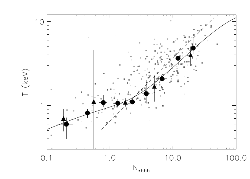
We summarize the general correlations in Figs. 7-12. We start with the correlations familiar from studies of X-ray clusters. Figure 7 shows the correlation between X-ray luminosity and temperature, Figure 8 show the relation between cluster mass and temperature, and Figure 9 shows the relation between entropy and temperature. In each case we show the results for the stacked clusters, the results of our global fit to the cluster properties (the “Poisson model”, except Fig. 9) and several similar scaling relations from the literature. In some cases we also show the measured properties of individual 2MASS clusters drawn from the literature (Ponman et al. 1996; Ebeling et al. 1996, 1998; De Grandi et al. 1999; Böhringer et al. 2000; Mahdavi et al. 2000; Cruddace et al. 2002; Reiprich & Böhringer 2002) and corrected to our assumed cosmology and to a bolometric X-ray luminosity.

The $L_{X}-T$ relation of the stacked clusters closely resembles that derived from observations of individual clusters (Fig. 7). There is a clear break in the slope between high and low temperature clusters. If we fit the results with a broken power law (see Table 3) we find slopes for rich ($2.7\pm 0.7$) and poor ($5.8\pm 1.7$) clusters consistent with studies of individual clusters ($2.5-3.0$ for rich clusters, Wu et al. 1999; Rosati et al. 2002 and $4-7$ for poor clusters, Helsdon & Ponman 2000; Xue & Wu 2000). The correlation we observe does not depend on the redshift when we subdivide our cluster catalogs into redshift bins. Similarly, the relationship between mass and temperature, shown in Fig. 8 for both $M_{200}$ and $M_{*666}$, is well-fit by a single power law with $M_{*666}\propto T^{1.79\pm 0.17}$ and $M_{200}\propto T^{1.59\pm 0.17}$ (see Table 3) The results are generally consistent with relations derived from samples of clusters (e.g. Xu et al. 2001; Neumann & Arnaud 1999; Sanderson et al. 2003; Arnaud et al. 2005b) as well as with theoretical models (Evrard et al. 1996). The offsets between $M_{*666}$ and $M_{200}$ created by the differences between $r_{*666}$ and $r_{200}$ discussed in §2.3 have little effect on the results. Finally, our estimated entropies are inconsistent with a simple $S\propto T$ scaling relation, as shown in Fig. 9. They are, however, consistent with the shallower $S\propto T^{0.65}$ relation of Ponman et al. (2003) or a break in the entropy for halos with the temperatures of order 1 keV where we observe a break in the $L_{X}-T$ relation. In summary, the X-ray properties of the stacked clusters are essentially indistinguishable from those found from studies of samples of individual clusters.

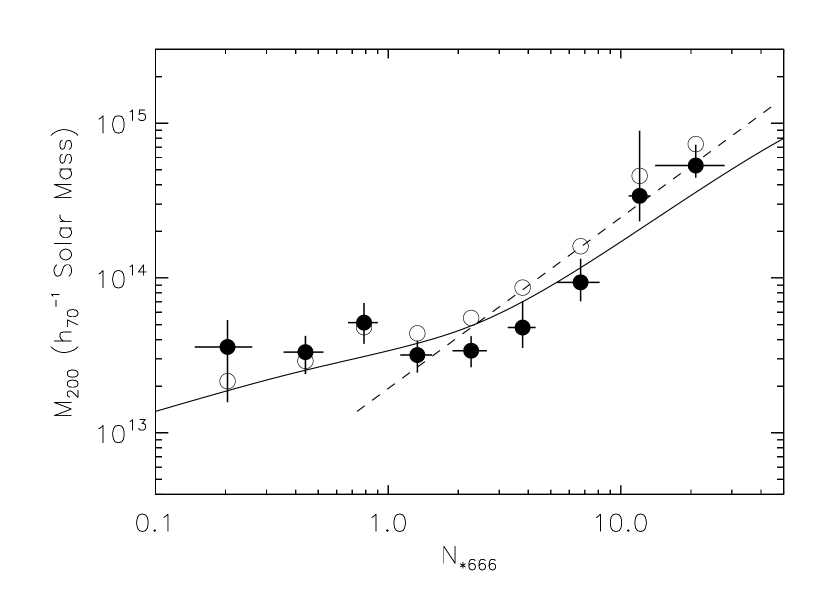
Figs. 10–12 show the correlations of the X-ray properties and the mass with the richness $N_{*666}$. At a first glance, these correlations may seem to be inconsistent with the X-ray and mass correlations we just discussed if the richness is a simple power-law of the mass (Eqn. 4). We carried out extensive tests to verify these correlations such as subdividing the sample by redshift, and using the soft-band rather than the bolometric luminosity. Using the soft-band luminosity avoids the need to accurately measure the temperature, and we expect any systematic problems in the richness estimate to be strongly redshift dependent. In fact, these correlations are the consequence of averaging at fixed optical richness in the presence of Poisson fluctuations. We can illustrate this by fitting all the correlations using the simple Poisson model of §3. We assume a power law relation for $T(M)$ and $N_{*666}(M)$, a broken power-law relation for $L_{X}(T)$, and a cluster mass function cutoff at mass scale $M_{0}$ over a mass range set by $\Delta$. Most of these parameters are simply the relations we need to fit the individual relations, with two parameters added to truncate the distribution of clusters at low mass. The parameters of these relations are summarized in Table 3, and we find a sensible mass cutoff of $\log M_{0}/M_{\odot}\simeq 13.46\pm 0.08$ that needs to be slightly softened by $\Delta\simeq 0.18\pm 0.03$ in order to reproduce the gradual decline in the X-ray temperatures and luminosities toward very low richness. The mass-richness relation is

$$\log N_{*666}=(1.10\pm 0.04)+(0.87\pm 0.05)\log(M/M_{1}).$$ (10)

Our earlier result in Kochanek et al. (2003) was that $\log N_{*666}=(1.44\pm 0.17)+(1.10\pm 0.09)\log(M/10^{15}M_{\odot})$ so the normalizations are consistent while the estimates of the slope differ by about $2\sigma$. The present, shallower slope is very similar to that of Lin, Mohr & Stanford (2004) or Popesso et al. (2005). Although the Poisson model is our preferred model, we also list the individual fits between stacked cluster properties in Table 3 for comparison with other studies.

Table 3: Fitting Results for $L_{X}$–$T_{X}$–$N_{*666}$–$M$.

Relation	Reference	Model	$\log{Y_{0}}$	$k$	$\log{X_{0}}$	$m$	$n$	$\chi^{2}_{\nu}(dof)$
Individual Fits
$L_{X}-T$	this paper	BPL	$43.11\pm 0.23$	$\cdots$	$0.13^{+0.59}_{-0.11}$	$2.7\pm 0.7$	$5.8\pm 1.7$	0.2(5)
$T-L_{X}$	this paper	BPL	$0.10\pm 0.04$	$\cdots$	$43.02\pm 0.7$	$0.37\pm 0.07$	$0.15\pm 0.07$	0.2(5)
$N_{*666}-L_{X}$	this paper	SPL	$0.43\pm 0.03$	$0.63\pm 0.04$	$43$	$\cdots$	$\cdots$	0.5(7)
	K03	SPL	$0.31\pm 0.06$	$0.75\pm 0.05$	$43$	$\cdots$	$\cdots$	$\cdots$
$L_{X}-N_{*666}$	this paper	SPL	$42.32\pm 0.07$	$1.56\pm 0.11$	$0$	$\cdots$	$\cdots$	0.5(7)
$N_{*666}-T$	this paper	SPL	$0.04\pm 0.04$	$2.26\pm 0.32$	$0$	$\cdots$	$\cdots$	1.5(7)
	K03	SPL	$-0.25\pm 0.14$	$2.09\pm 0.17$	$0$	$\cdots$	$\cdots$	$\cdots$
	this paper	BPL	$0.56\pm 0.13$	$\cdots$	$0.13\pm 0.13$	$1.35\pm 0.42$	$4.0\pm 1.2$	0.4(5)
$T-N_{*666}$	this paper	SPL	$-0.01\pm 0.03$	$0.36\pm 0.06$	$0$	$\cdots$	$\cdots$	1.4(7)
	this paper	BPL	$0.09\pm 0.04$	$\cdots$	$0.51\pm 0.27$	$0.74\pm 0.17$	$0.20\pm 0.07$	0.4(5)
$M_{*666}-T$	this paper	SPL	$13.64\pm 0.05$	$1.79\pm 0.17$	$0$	$\cdots$	$\cdots$	0.1(7)
$M_{200}-T$	this paper	SPL	$13.56\pm 0.05$	$1.59\pm 0.17$	$0$	$\cdots$	$\cdots$	1.0(7)
$M_{*666}-N{*666}$	this paper	SPL	$13.64\pm 0.06$	$0.74\pm 0.10$	$0$	$\cdots$	$\cdots$	1.1(7)
	this paper	BPL	$13.79\pm 0.09$	$\cdots$	$0.48\pm 0.30$	$1.27\pm 0.28$	$0.36\pm 0.17$	0.1(5)
$M_{200}-N{*666}$	this paper	SPL	$13.58\pm 0.06$	$0.56\pm 0.10$	$0$	$\cdots$	$\cdots$	2.9(7)
	this paper	BPL	$13.53\pm 0.09$	$\cdots$	$0.49\pm 0.18$	$1.44\pm 0.27$	$-0.05\pm 0.17$	0.1(5)
Poisson Model Fits
$L_{X}-T$	this paper	BPL	$42.55\pm 0.05$	$\cdots$	$0.00\pm 0.05$	$3.03\pm 0.17$	$10.3\pm 2.4$	$\cdots$
$M_{200}-T$	this paper	SPL	$13.58\pm 0.05$	$1.65\pm 0.12$	$0$	$\cdots$	$\cdots$	$\cdots$

Note. — The single power law (SPL) is defined by $Y=Y_{0}(X/X_{0})^{k}$ while the broken power law (BPL) is $Y=Y_{0}(X/X_{0})^{m}$ for $X>X_{0}$ and $Y=Y_{0}(X/X_{0})^{n}$ for $X<X_{0}$.

The last point we consider is whether the matched filter algorithm leads to cluster catalogs with redshift-dependent biases. We test for the biases by dividing each richness bin into three redshift bins with the boundaries chosen so that each bin produced a stacked spectrum with a similar signal-to-noise ratio. We also created two overlapping (i.e. not independent) redshift bins centered on the edges of the first sets of bins to better illustrate any variations with redshift. For each of these bins we extracted the spectra as described in §4, normalized each spectrum to the mean redshift of the bin, fit the spectra to obtain the luminosity and temperature and estimated the uncertainties using bootstrap re-sampling. The results are shown in Figures 13 and 14, either as the raw results or normalized to remove the variations in the mean richness between the redshift bins. The error-bars for temperatures are larger than those for the luminosities and we only show results from the first three richness bins.

The qualitative result is that there are few signs of redshift dependent biases beyond the expectations of the Poisson model. The most massive clusters (richnesses 0 and 1) show a slow decline in the mean luminosity and temperature at fixed richness because of the increase in the Malmquist biases with the diminishing numbers of detectable galaxies. The intermediate richness class 1 is far enough from both the break in the mass function and the lower mass limit to show little variation with redshift. The two lowest richness classes show a rapidly rising luminosity with redshift. In all cases, the trends are well matched by the simple Poisson model – we see no evidence for additional systematic biases.

Figure 13: X-ray luminosity versus redshift for stacked clusters in richness bins 0 (top) to 4 (bottom). The upper panel shows the raw results, the lower panel corrects for the difference between the mean richness of all clusters in the richness bin and the mean richness in the individual redshift bins. The even and odd points in the redshift sequences are not independent measurements. The lines in both panels are the best fit Poisson models for each richness bin.

Figure 14: Temperature versus redshift for stacked clusters in richness bins 0 (top), 1, and 2 (bottom). The upper panel shows the raw results, the lower panel corrects for the difference between the mean richness of all clusters in the richness bin and the mean richness in the individual redshift bins. The even and odd points in the redshift sequences are not independent measurements. The lines in both panels are the best fit Poisson models for each richness bin.

5 Summary

Optically-selected cluster catalogs have always been suspect because of concerns about false detections and redshift-dependent biases created by chance alignments of galaxies. Current attempts to understand the biases of optically-selected catalogs have focused either on testing the algorithms in mock galaxy catalogs (Kochanek et al. 2003; Miller et al. 2005) or by using weak lensing measurements (Sheldon et al. 2001). Unfortunately, there has never been a complete X-ray survey of a large optically-selected cluster catalog to provide an independent test of these concerns. In this study we have used a stacking analysis of the ROSAT All-Sky Survey data to determine the average X-ray properties of a sample of 4333 clusters found using the matched filter algorithm of Kochanek et al. (2003) applied to the 2MASS galaxy survey with a magnitude limit of K$<13.25$ mag.

After dividing the clusters into bins of optical richness, we could successfully measure the surface brightness profiles, bolometric X-ray luminosities, X-ray temperatures, masses and gas entropies for the averaged clusters, finding results that are generally consistent with those from analyzing individual clusters. The one exception is that we tend to find larger core radii for $\beta$-model fits to the surface brightness presumably because of additional smoothing created by errors in the optical positions. The stacked clusters cleanly follow the correlations observed for samples of individual clusters between X-ray luminosity, temperature and mass. However, in order to interpret the correlations between the optical richness and the X-ray luminosity, temperature and mass, it is necessary to model the effects of Poisson fluctuations of the number of galaxies in a cluster because in the presence of these fluctuations averaging at fixed richness is very different from averaging at fixed mass. These effects matter for high richness clusters observed at redshifts where they will contain few detectable galaxies, and for all low richness clusters. A very simple Poisson model for the effects of these fluctuations naturally reproduces our results. We note that Stanek et al. (2006) have recently demonstrated similar effects arising from the scatter in X-ray luminosity at fixed cluster mass.

We also examined the problem of redshift-dependent biases in optical catalogs by examining the X-ray properties of clusters of fixed richness as a function of redshift. The low redshifts of the 2MASS clusters ($z<0.1$) means that we need worry little about genuine cosmological evolution. Our statistical model predicts that high richness clusters will show a slowly declining X-ray luminosity, while low richness clusters will show a rising X-ray luminosity, and this agrees with our measurements. Essentially, Malmquist biases created by the much more abundant low-mass clusters become steadily more important for the high mass clusters as the numbers of detectable member galaxies decline, while the reverse occurs for the low-mass clusters. In general, however, samples restricted to clusters containing at least 3 detectable galaxies (already a floor required to minimize the abundance of false positives) and to the higher mass clusters rather than groups ($T\lower 2.0pt\hbox{$\;\scriptscriptstyle\buildrel>\over{\sim}\;$}2$ keV, $M\lower 2.0pt\hbox{$\;\scriptscriptstyle\buildrel>\over{\sim}\;$}10^{14}M_{\odot}$, $L_{X}\lower 2.0pt\hbox{$\;\scriptscriptstyle\buildrel>\over{\sim}\;$}10^{43}$ ergs/sec) have corrections due to the effects of Poisson fluctuations that are relatively simple to model and depend little on the model for the cutoff between groups and galaxies. Models for the lower mass groups are more challenging, particularly if variations with redshift must be included. We see no evidence for large systematic errors created by chance superpositions.

Despite the shallowness of the RASS, our approach (see also Bartelmann & White 2003) can be applied to analyses of cluster samples with much higher mean redshifts than the 2MASS sample, where even the richest clusters are tracked only to $z\lower 2.0pt\hbox{$\;\scriptscriptstyle\buildrel<\over{\sim}\;$}0.1$. Modulo redshift scalings for K-corrections and between cosmological distances, the signal-to-noise ratio of a stacking analysis scales as the square root of the product of the survey area and depth. Thus, an analysis of clusters in 10000 deg² of the SDSS survey (25% of the area of 2MASS), which can detect rich clusters with $z\lower 2.0pt\hbox{$\;\scriptscriptstyle\buildrel<\over{\sim}\;$}0.5$ rather than $z\lower 2.0pt\hbox{$\;\scriptscriptstyle\buildrel<\over{\sim}\;$}0.1$ (5 times the depth), should have a signal-to-noise ratio comparable to our present analysis for the measurement of the mean X-ray properties of the clusters. Analyses of rich clusters over 1000 deg² would have a signal-to-noise ratio comparable to our analysis of clusters with $\sim 1/3$ the richness. This assumes that the analysis remains limited by statistical errors rather than being dominated by systematic problems such as contamination by faint point sources or difficulty in controlling the background.

References

- Abell (1958) Abell, G. O. 1958, ApJS, 3, 211
- Adami et al. (1998) Adami, C., Mazure, A., Katgert, P., & Biviano, A. 1998, A&A, 336, 63
- Arnaud (1996) Arnaud, K. A. 1996, ASP Conf. Series Vol. 101: Astronomical Data Analysis Software and Systems V, ed. Jacoby G. & Barnes J., 17
- Arnaud (2005a) Arnaud, M. 2005a, astro-ph/0508159
- Arnaud et al. (2005b) Arnaud, M., Pointecouteau, E., & Pratt, G. W. 2005b, A&A, 441, 893
- Bahcall (1977) Bahcall, N. A. 1977, ApJ, 218, L93
- Bahcall et al. (2003) Bahcall, N. A., et al. 2003, ApJS, 148, 243
- Bartelmann & White (2003) Bartelmann, M. & White, S. D. M. 2003, A&A, 407, 845
- Bauer et al. (2002) Bauer, F. E., et al. 2002, AJ, 123, 1163
- Baumgartner et al. (2005) Baumgartner, W. H., Loewenstein, M., Horner, D. J., & Mushotzky, R. F. 2005, ApJ, 620, 680
- Berlind & Weinberg (2002) Berlind, A. A. & Weinberg, D. H. 2002, ApJ, 575, 587
- Bower et al. (1997) Bower, R. G., Castander, F. J., Ellis, R. S., Couch, W. J., & Böhringer, H. 1997, MNRAS, 291, 353
- Böhringer et al. (2000) Böhringer, H., et al. 2000, ApJS, 129, 435
- Böhringer et al. (2004) Böhringer, H., et al. 2004, A&A, 425, 367
- Bregman & Lloyd-Davies (2006) Bregman, J. N. & Lloyd-Davies, E. J. 2006, ApJ, 644, 167
- Carlstrom et al. (2000) Carlstrom, J. E., et al. 2000, Phys. Scr., 85, 148
- Cruddace et al. (2002) Cruddace, R., et al. 2002, ApJS, 140, 239
- Dahle et al. (2002) Dahle, H., Kaiser, N., Irgens, R. J., Lilje, P. B., & Maddox, S. J. 2002, ApJS, 139, 313
- Dalton et al. (1992) Dalton, G. B., Efstathiou, G., Maddox, S. J., & Sutherland, W. J. 1992, ApJ, 390, L1
- De Grandi et al. (1999) De Grandi, S., et al. 1999, ApJ, 514, 148
- Donahue et al. (2002) Donahue, M., et al. 2002, ApJ, 569, 689
- Ebeling et al. (1996) Ebeling, H., Voges, W., Böhringer, H., Edge, A. C., Huchra, J. P., & Briel, U. G. 1996, MNRAS, 281, 799
- Ebeling et al. (2000) Ebeling, H., Edge, A. C., Allen, S. W., Crawford, C. S., Fabian, A. C. & Huchra, J. P. 2000, MNRAS, 318, 333
- Ebeling et al. (1998) Ebeling, H., Edge, A. C., Böhringer, H., Allen, S. W., Crawford, C. S., Fabian, A. C., Voges, W., & Huchra, J. P. 1998, MNRAS, 301, 881
- Ebeling, Edge, & Henry (2001) Ebeling, H., Edge, A. C., & Henry, J. P. 2001, ApJ, 553, 668
- Evrard et al. (1996) Evrard, A. E., Metzler, C. A., Navarro, J. F. 1996, ApJ, 469, 494
- Gal et al. (2003) Gal, R. R., de Carvalho, R. R., Lopes, P. A. A., Djorgovski, S. G., Brunner, R. J., Mahabal, A., & Odewahn, S. C. 2003, AJ, 125, 2064
- Giacconi et al. (2002) Giacconi, R., et al. 2002, ApJS, 139, 369
- Gilbank et al. (2004) Gilbank, D. G., Bower, R. G., Castander, F. J. & Ziegler, B. L. 2004, MNRAS, 348, 551
- Gioia et al. (1990) Gioia, I. M., Henry, J. P., Maccacaro, T., Morris, S. L., Stocke, J. T., & Wolter, A. 1990, ApJ, 356, L35
- Gladders & Yee (2005) Gladders, M. D. & Yee, H. K. C. 2005, ApJS, 157, 1
- Gonzalez et al. (2001) Gonzalez, A. H., Zaritsky, D., Dalcanton, J. J., & Nelson, A. 2001, ApJS, 137, 117
- Goto et al. (2002) Goto, T., et al. 2002, AJ, 123, 1807
- Haiman, Mohr, & Holder (2001) Haiman, Z., Mohr, J. J., & Holder, G. P. 2001, ApJ, 553, 545
- Hasinger et al. (2001) Hasinger, G., et al. 2001, A&A, 365, L45
- Helsdon & Ponman (2000) Helsdon, S. F., & Ponman, T. J. 2000, MNRAS, 319, 933
- Henry et al. (1992) Henry, J. P., Gioia, I. M., Maccacaro, T., Morris, S. L., Stocke, J. T., & Wolter, A. 1992, ApJ, 386, 408
- Horner, Mushotzky, & Scharf (1999) Horner, D. J., Mushotzky, R. F., & Scharf, C. A. 1999, ApJ, 520, 78
- Hu (2003) Hu, W. 2003, PhRvD, 67, 081304
- Huchra & Geller (1982) Huchra, J. P. & Geller, M. J. 1982, ApJ, 257, 423
- Huterer & Turner (2001) Huterer, D. & Turner, M. S. 2001, PhRvD, 64, 123527
- Kneissl et al. (2001) Kneissl, R., Jones, M. E., Saunders, R., Eke, V. R., Lasenby, A. N., Grainge, K., Cotter, G. 2001, MNRAS, 328, 783
- Kochanek et al. (2001) Kochanek, C. S., et al. 2001, ApJ, 560, 566
- Kochanek et al. (2003) Kochanek, C. S., White, M., Huchra, J., Macri, L., Jarrett, T. H., Schneider, S. E., & Mader, J. 2003, ApJ, 585, 161
- LaRoque et al. (2003) LaRoque, S. J., et al. 2003, ApJ, 583, 559
- Levine, Schulz, & White (2002) Levine, E. S., Schulz, A. E., & White, M. 2002, ApJ, 577, 569
- Lin (2004) Lin, Y. T., Mohr, J. J. & Stanford, S. A. 2004, ApJ, 610, 745
- Lloyd-Davies, Ponman, & Cannon (2000) Lloyd-Davies, E. J., Ponman, T. J., & Cannon, D. B. 2000, MNRAS, 315, 689
- Lopes et al. (2006) Lopes, P. A. A., de Carvalho, R. R., Capelato, H. V., Gal, R. R., Djorgovski, S. G., Brunner, R. J., Odewahn, S. C., & Mahabal, A. A. 2006, astro-ph/0605292
- Lubin, Mulchaey & Postman (2004) Lubin, L. M., Mulchaey, J. S., & Postman, M. 2004, ApJL, 601, L19
- Mahdavi et al. (2000) Mahdavi, A., Böhringer, H., Geller, M. J., & Ramella, M. 2000, ApJ, 534, 114
- Majumdar & Mohr (2003) Majumdar, S. & Mohr, J. J. 2003, ApJ, 585, 603
- Miller et al. (2005) Miller, C. J., et al. 2005, AJ, 130, 968
- Neumann & Arnaud (1999) Neumann, D. M. & Arnaud, M. 1999, A&A, 348, 711
- Newman et al. (2002) Newman, J. A., Marinoni, C., Coil, A. L., & Davis, M. 2002, PASP, 114, 29
- Osmond & Ponman (2004) Osmond, J. P. F. & Ponman, T. J. 2004, MNRAS, 350, 1511
- Ostrander et al. (1998) Ostrander, E. J., Nichol, R. C., Ratnatunga, K. U., & Griffiths, R. E. 1998, AJ, 116, 2644
- Podariu & Ratra (2001) Podariu, S. & Ratra, B. 2001, ApJ, 563, 28
- Ponman et al. (1996) Ponman, T. J., Bourner, P. D. J., Ebeling, H., & Böhringer, H. 1996, MNRAS, 283, 690
- Ponman, Cannon, & Navarro (1999) Ponman, T. J., Cannon, D. B., & Navarro, J. F. 1999, Nature, 397, 135
- Ponman, Sanderson, & Finoguenov (2003) Ponman, T. J., Sanderson, A. J. R., & Finoguenov, A. 2003, MNRAS, 343,331
- Popesso et al. (2004) Popesso, P., Böhringer, H., Brinkmann, J., Voges, W., & York, D.G. 2004, A&A, 423, 449
- (63) Popesso, P., Biviano, A., Böhringer, H., Romaniello, M., & Voges, W. 2005, A&A, 433, 431
- Postman et al. (2002) Postman, M., Lauer, T. R., Oegerle, W., & Donahue, M. 2002, ApJ, 579, 93
- Postman et al. (1996) Postman, M., Lubin, L. M., Gunn, J. E., Oke, J. B., Hoessel, J. G., Schneider, D. P., & Christensen, J. A. 1996, AJ, 111, 615
- Raymond & Smith (1977) Raymond, J. C. & Smith, B. W. 1977, ApJS, 35, 419
- Reiprich & Böhringer (2002) Reiprich, T. H., Böhringer, H. 2002, ApJ, 567, 716
- Rosati, Borgani, & Norman (2002) Rosati, P., Borgani, S. & Norman, C. 2002, ARA&A, 40, 539
- Rosati et al. (1995) Rosati, P., della Ceca, R., Burg, R., Norman, C. & Giacconi, R. 1995, ApJ, 445, L11
- Rosati et al. (1998) Rosati, P., della Ceca, R., Norman, C. & Giacconi, R. 1998, ApJ, 492, L21
- Sanderson et al. (2003) Sanderson, A. J. R., Ponman, T. J., Finoguenov, A., Lloyd-Davies, E. J., & Markevitch, M. 2003, MNRAS, 340, 989
- Schirmer et al. (2003) Schirmer, M., Erben, T., Schneider, P., Pietrzynski, G., Gieren, W., Carpano, S., Micol, A., & Pierfederici, F. 2003, A&A, 407, 869
- Scodeggio et al. (1999) Scodeggio, M., Olsen, L. F., da Costa, L., Slijkhuis, R., Benoist, C., Deul, E., Erben, T., Hook, R., Nonino, M., Wicenec, A., & Zaggia, S. 1999, A&AS, 137, 83
- Sheldon et al. (2001) Sheldon, E. S., et al. 2001, ApJ, 554, 881
- Skrutskie et al. (2006) Skrutskie, M. F., et al. 2006, AJ, 131, 1163
- Stanek et al. (2006) Stanek, R., Evrard, A. E., Böhringer, H., Schuecker, P., & Nord, B. 2006, ApJ in press [astro-ph/0602324]
- Voges et al. (1999) Voges, W., et al. 1999, A&A, 349, 389
- White & Kochanek (2002) White, M., & Kochanek, C. S. 2002, ApJ, 574, 24
- White et al. (1999) White, R. A., Bliton, M., Bhavsar, S. P., Bornmann, P., Burns, J. O., Ledlow, M. J., & Loken, C. 1999, AJ, 118, 2014
- Wittman et al. (2001) Wittman, D., et al. 2001, ApJ, 557, L89
- Wu, Xue, & Fang (1999) Wu, X.-P., Xue, Y.-J., & Fang, L.-Z. 1999, ApJ, 524, 22
- Xu, Jin, & Wu (2001) Xu, H., Jin, G., & Wu, X.-P. 2001, ApJ, 553, 78
- Xue & Wu (2000) Xue, Y.-J. & Wu, X.-P. 2000, ApJ, 538, 65
- Yang et al. (2005) Yang, X., Mo, H. J., Jing, Y. P., & van den Bosch, F. C. 2005, MNRAS, 358, 217
- Zaritsky et al. (1997) Zaritsky, D., Nelson, A. E., Dalcanton, J. J., & Gonzalez, A. H. 1997, ApJ, 480, L91
- Zheng et al. (2005) Zheng, Z., Berlind, A. A., Weinberg, D. H., Benson, A. J., Baugh, C. M., Cole, S., Davé, R., Frenk, C. S., Katz, N., & Lacey, C. G. 2005, ApJ, 633, 791