Accretion, feedback and galaxy bimodality: a comparison of the GalICS semi-analytic model and cosmological SPH simulations

Abstract

We compare the galaxy population of a smoothed particle hydrodynamics (SPH) simulation to those predicted by the GalICS N-body + semi-analytic model and a stripped down version of GalICS that omits supernova and AGN feedback. The SPH simulation and the no-feedback GalICS model make similar predictions for the baryonic mass functions of galaxies and for the dependence of these mass functions on environment and redshift. The two methods also make similar predictions for the galaxy content of dark matter haloes as a function of halo mass and for the gas accretion history of galaxies. There is a fairly good correspondence between the “cold” and “hot” accretion modes of the SPH simulation and the rapid and slow cooling regimes of the GalICS calculation. Both the SPH and no-feedback GalICS models predict a bimodal galaxy population at $z=0$. The “red” sequence of gas poor, old galaxies is populated mainly by satellite systems, which are starved of fresh gas after they begin orbiting in larger haloes, while, contrary to observations, the central galaxies of massive haloes lie on the “blue” star-forming sequence as a result of continuing hot gas accretion at late times. Furthermore, both models overpredict the observed baryonic mass function, especially at the high mass end. In the full GalICS model, supernova-driven outflows reduce the masses of low and intermediate mass galaxies by about a factor of two. AGN feedback suppresses gas cooling in large haloes, producing a sharp cut-off in the baryonic mass function and moving the central galaxies of these massive haloes to the red sequence. Our results imply that the observational failings of the SPH simulation and the no-feedback GalICS model are a consequence of missing input physics rather than computational inaccuracies, that truncating gas accretion by satellite galaxies automatically produces a bimodal galaxy distribution with a red sequence, but that explaining the red colours of the most massive galaxies requires a mechanism like AGN feedback that suppresses the accretion onto central galaxies in large haloes.

1 Introduction

The classification of galaxies into early-type and late-type goes back to the earliest studies (Hubble, 1926; Humason, 1936), but the clear demonstration that there is no smooth continuity between the two types was only possible with the advent of large statistical surveys (Strateva et al., 2001; Kauffmann et al., 2003; Baldry et al., 2004; Balogh et al., 2004; Hogg et al., 2004; also see Dekel & Birnboim 2006 for a comprehensive introduction to the bimodality problem). Galaxy colour-magnitude diagrams from the Sloan Digital Sky Survey (SDSS) show a clear distinction between a tight red sequence with no recent star formation and a broader blue sequence, where star formation is still going on. The blue sequence is truncated near the characteristic luminosity $L_{*}$ of the Schechter (1976) luminosity function, while the red sequence extends to luminosities several times higher. Elliptical galaxies concentrate in the bright part of the red sequence ($L\mathrel{\hbox{\hbox to0.0pt{\hbox{\lower 4.0pt\hbox{$\sim$}}\hss}\hbox{$>$}}}L_{*}$). Galaxies in crowded environments are normally red, while blue galaxies reside mainly in the field (Kauffmann et al., 2003; Blanton et al., 2005; and numerous references therein). Deep surveys like COMBO-17 and DEEP-2 show that bimodality is already well established at $z\sim 1$ (Bell et al., 2004; Faber et al., 2005), and even at $z\ga 3$ there appears to be a distinction between actively star-forming galaxies and passive systems dominated by redder stellar populations (e.g., van Dokkum et al., 2006). Here we investigate the physical origin of this bimodality in the context of modern galaxy formation theory, comparing the results of two different modelling methods.

Cosmological hydrodynamic simulations (see Frenk et al., 1999 for a review), which integrate the equations of motions for the baryons alongside those for the dark matter, and hybrid simulations, which combine an N-body treatment of the dark matter with semi-analytic modelling of the baryons (e.g. Yoshida et al., 2002; Hatton et al., 2003; Helly et al., 2003; De Lucia et al., 2004; Croton et al., 2005; Cattaneo et al., 2006), are the main methods for exploring the physics of galaxy formation in a cosmological scenario while retaining the spatial information on the galaxy distribution. The fully numerical approach treats the dynamics and the gas physics more self-consistently because accretion and mergers come out naturally from the physics of the simulations. In the hybrid approach, the same phenomena are modelled through assumptions, such as the hypothesis that the gas starts cooling from a spherical distribution at the virial temperature of the halo or the dynamical friction formula to compute merging rates. However, hydrodynamic simulations are expensive in CPU time. That limits the resolution mass and the size of the computational box, the latter resulting in poor sampling of rare objects. It also means that, for the same CPU time, hybrid methods allow one to explore a wider set of physical assumptions, such as different feedback scenarios. In this paper, we compare results from a smoothed particle hydrodynamics (SPH) simulation (Katz et al., 1996) to those of the GalICS hybrid model (Galaxies In Cosmological Simulations; Hatton et al., 2003).

This comparison tests the consistency between the gas dynamical treatment of the SPH simulation and the idealised model incorporated in GalICS, since we run GalICS with merger trees extracted from the SPH simulation itself. Two groups, centred in Durham (Benson et al., 2001; Helly et al., 2003) and Munich (Yoshida et al., 2002), have already performed similar checks, verifying that the two semi-analytic models investigated (Cole et al., 2000; Kauffmann et al., 1999) predict galaxy masses and luminosity functions in reasonable agreement with cosmological SPH simulations run with the HYDRA (Pearce et al., 2001) and GADGET (Springel et al., 2001) codes, when the physical assumptions are similar. One motivation for our study was simply to conduct the same test for GalICS. However, we also focus on issues related to the galaxy bimodality, such as the distinction between central and satellite galaxies and the possible connection to the distinction between “cold” and “hot” gas accretion (Katz et al., 2003; Birnboim & Dekel, 2003; Kereš et al., 2005; Dekel & Birnboim, 2006). To illuminate these issues, we consider two versions of the GalICS model: a “stripped-down” version with no feedback, designed to approximately match the physics of the SPH simulation, and the full version described by Hatton et al. (2003) and used in Blaizot et al. (2004), Lanzoni et al. (2005) and Cattaneo et al. (2005), which contains supernova and AGN feedback prescriptions designed to reproduce the blue luminosity function of galaxies. We show that the SPH simulation and the no-feedback GalICS model produce a red sequence of satellite galaxies in massive haloes, but predict, contrary to observations, that the central galaxies of massive haloes lie on the blue sequence. The strong supernova feedback incorporated in the full GalICS model reduces galaxy baryonic masses to a level consistent with observations. The combination of supernova and (more importantly) AGN feedback shuts off gas accretion in massive central galaxies, turning them red.

Section 2 describes the astrophysical and computational assumptions used in the SPH simulation together with the algorithms used to identify galaxies and haloes, to attribute galaxies to haloes, and to construct merger trees by linking haloes identified at different time-steps. Section 3 summarises the GalICS implementation used here, in particular its assumptions about gas accretion, star formation and feedback. In Section 4 we begin our comparison of the two methods with a global view of the model galaxy populations. We investigate the mass function, its dependence on redshift and environment, and the relation between galaxies and dark matter haloes. We then move into more specific aspects such as the growth mechanism (cold flows versus hot flows; Section 5), the gas content, and the presence (or absence) of a bimodality in the distributions of gas content and star formation time-scales (Section 6). In Section 7, we discuss how this work contributes to our understanding of galaxy formation and of the processes that are at the basis of the observed galaxy bimodality. Section 8 summarises our results.

2 The SPH simulation

2.1 Cosmological model and simulation parameters

The cosmology used for this study is a flat $\Lambda$CDM universe (inflationary cold dark matter with a cosmological constant) with $h\equiv H_{0}/(100{\rm\,km\,s^{-1}\,Mpc^{-1}})=0.65$, $\Omega_{m}=0.4$, $\Omega_{\Lambda}=0.6$, $\Omega_{b}=0.02h^{-2}=0.0473$, inflationary spectral index $n=0.93$, and power spectrum normalisation $\sigma_{8}=0.8$. We have used this combination of parameters in a series of simulations over the course of a number of years (beginning with Davé et al., 1999), systematically varying numerical resolution and simulation volume. The values of $h$, $\Omega_{b}$, $n$, and $\sigma_{8}$ are similar to those inferred from joint analyses of cosmic microwave background (CMB) measurements from the WMAP satellite and galaxy power spectrum measurements from the 2dF Galaxy Redshift Survey and the SDSS (e.g., Spergel et al., 2003; Tegmark et al., 2004; Sánchez et al., 2006). These analyses generally favour a lower $\Omega_{m}$ value, in the range $\sim 0.23-0.3$, but the qualitative features of galaxy formation are not sensitive to the precise value of $\Omega_{m}$ (a point we have checked by running a comparable simulation with $\Omega_{m}=0.3$). Since we adopt identical parameters for the SPH and GalICS modelling, this simulation should be entirely adequate for our purposes in this paper, despite its slightly outdated parameter values.

The simulation volume is a comoving periodic cube $22.22h^{-1}=34.19$ Mpc on a side, modelled using $128^{3}$ dark matter particles and $128^{3}$ gas particles. Gravitational forces are softened with a cubic spline kernel of comoving radius $7.7\,$kpc, approximately equivalent to a Plummer force softening of $\epsilon_{\rm grav}=5.4\,$kpc, while hydrodynamic pressure forces are calculated over 32 neighbours. The baryonic mass threshold for resolved galaxies is $6.8\times 10^{9}M_{\odot}$, the mass of 64 gas particles, and there are 1120 galaxies in the box above this threshold at $z=0$. Further details of the simulation can be found in Kereš et al. (2005).

2.2 The SPH code

The simulation was performed with the parallel version of TreeSPH (Hernquist & Katz 1989; Katz et al. 1996; Dave et al. 1997). This code combines smoothed particle hydrodynamics (SPH; Lucy 1977; Gingold & Monaghan 1977) with a hierarchical tree algorithm for computing gravitational forces (Barnes & Hut, 1986; Hernquist, 1987). TreeSPH is a completely Lagrangian code, adaptive both in space and in time. It contains three kinds of particles, representing dark matter, gas and stars. The dark matter and the stars are only subject to gravity, while the gas is also subject to pressure gradients and shocks. The gas experiences adiabatic heating and cooling, shock heating, inverse Compton cooling off the microwave background and radiative cooling via free-free emission, collisional ionisation, collisional recombination, and collisionally excited line cooling. The cooling rate is calculated for primordial chemical abundances and, since there is only atomic cooling, the gas cannot cool radiatively below $T\sim 10^{4}\,$K. A uniform photoionising UV background heats low temperature gas and suppresses cooling processes involving neutral atoms at low gas densities (Haardt & Madau, 1996).

The simulation also includes a simple treatment of star formation and its associated supernova feedback. Gas above a threshold hydrogen number density $n_{H}=0.1{\rm cm}^{-3}$ turns into stars on a time-scale set by the dynamical time or the cooling time, whichever is longer. Additional star formation conditions are that the gas is Jeans unstable, part of a converging flow and above the virial overdensity, but gas that satisfies the density criterion usually also satisfies the other three. Gas reaches this high density only after cooling to $T\sim 10^{4}\,$K. The subsequent molecular and metal-line cooling to lower temperatures is implicitly included as part of the star formation process. This star formation prescription leads to a relation with the gas surface density similar to a Schmidt law (Schmidt, 1959; Kennicutt, 1998; see discussions by Katz et al., 1996 and Stinson et al., 2006).

Stars more massive than $8M_{\odot}$ explode as supernovae. For a Miller & Scalo (1979) initial mass function that means $7.35\times 10^{-3}$ supernovae per solar mass of formed stars. Each supernova releases $10^{51}\,$erg, gradually distributed as heat to the gas particles nearby with an exponential time decay of $2\times 10^{7}\,$yr. The surrounding medium is usually dense, so the deposited energy is typically radiated away before it can drive a galactic scale wind. For this reason, we consider this a “minimal” feedback algorithm, even though the full amount of expected supernova energy is incorporated.

2.3 Identification of galaxies

Cosmological simulations that incorporate cooling and star formation produce dense groups of baryonic particles with the sizes and masses of observed galaxies (Katz, 1992; Evrard et al., 1994). We identify these aggregations with the group finding algorithm ‘Spline Kernel Interpolative DENMAX’ (SKID) (Gelb & Bertschinger, 1994; Katz et al., 1996). This algorithm involves five basic steps: (1) determining the smoothed baryonic density field; (2) moving baryonic particles towards higher density along the initial gradient of the baryonic density field; (3) defining the initial group as a set of particles that aggregate at a particular density peak; (4) linking together initial groups that are very close together; (5) removing group particles with positive binding energy relative to the group’s centre of mass. We apply SKID to the population of all star particles and to the gas particles that have temperatures $T<3\times 10^{4}\,$K and overdensities $\rho_{\rm gas}/{\bar{\rho}}_{\rm gas}>10^{3}$. Henceforth, we refer to the aggregations of stars and cold gas that SKID identifies simply as “galaxies.” Tests on simulations with varying mass resolution show that the simulated galaxy population becomes substantially incomplete below a baryonic mass corresponding to $\sim 64m_{\rm SPH}$ but is fairly robust above this limit (see, e.g., Murali et al. 2002). We therefore adopt $64m_{\rm SPH}$ ($6.8\times 10^{9}M_{\odot}$) as our resolution threshold and ignore lower mass galaxies in our analysis. Because of our high overdensity threshold for star formation, essentially all star formation in the simulation takes place in galaxies, though some of these are below the resolution limit, and some stars are tidally stripped from galaxies during dynamical interactions.

The minimum galaxy mass of $64m_{\rm SPH}$ corresponds to a minimum host halo mass of $\sim(\Omega_{m}/\Omega_{b})64m_{\rm SPH}$, since the fraction of cold gas in a halo never substantially exceeds the universal baryon fraction. The corresponding minimum virial temperature for our simulation is $\sim 80,000(1+z)\,$K for the simulation considered in this article, where the $(1+z)$ factor arises from the increasing physical density at higher $z$ for fixed virial overdensity. The redshift dependence of the virial overdensity makes the ‘$80,000\,$K’ factor slightly lower at high redshift ($\sim 75,000\,$K) and slightly higher at low redshift ($88,000\,$K at $z=0$). Any resolved galaxy in the simulation resides in a dark matter halo with virial temperature higher than this minimum temperature.

3 The GalICS hybrid model

The semi-analytic model that we use in this paper is exactly the one described in Hatton et al. (2003). In this section, we therefore only briefly summarise those of its features which are relevant to the present study.

3.1 Dark matter haloes and their merger trees

We identify and characterise dark matter haloes the same way as in Hatton et al. (2003). We use a friends-of-friends (FOF) algorithm (Davis et al., 1985) to detect groups of particles with overdensity $\sim 200$ times the mean density (using a fixed linking-length parameter $b=0.2$). For each group with more than 20 particles, we compute the total kinetic and potential energies, and only keep in the halo catalogue the groups that are bound. The halo mass we refer to in the rest of the paper is simply $N_{p}\times m_{p}$, where $N_{p}$ is the number of particles in the group, and $m_{p}$ the mass of a dark matter particle. The minimum halo mass is thus $\sim 1.8\times 10^{10}M_{\odot}$. We set the centres of groups to be at the positions of their centres of mass.

The information about an individual halo measured from the SPH outputs and passed to the semi-analytic model is contained in three parameters: the virial mass, the spin parameter, and the virial radius. The virial mass and the virial radius are measured in two steps. First, we compute the inertia tensor of each halo. From this we determine the three main axes of an ellipsoid that fits the mass distribution and is centred on the centre of mass. Then we shrink this ellipsoid until the halo particles that it contains satisfy the virial theorem. The mass of the particles in the ellipsoid at this point is the virial mass. The virial radius is the radius of a sphere with the same volume as the virial ellipsoid.

We compute merger trees by linking haloes identified in each SPH snapshot with their progenitors in the previous one. All predecessors from which a halo has inherited one or more particles are counted as progenitors.

3.2 The cooling scheme

Newly identified haloes receive a gas mass determined by the universal baryonic fraction $\Omega_{b}/\Omega_{m}$. As in other semi-analytic models, all baryons start in a zero-metallicity hot phase, shock-heated to the virial temperature. We assume that the the hot gas density profile is described by a singular isothermal sphere truncated outwards at the virial radius and inwards at a core radius of 0.1 kpc.

The cooling time $t_{\rm cool}(r)$ is calculated from the hot gas density distribution with the metal-dependent cooling function from Sutherland & Dopita (1993). There are two differences with the SPH calculation here. First, the semi-analytic calculation does not include a photoionising background, although photoionisation effects on galaxy formation are small in the halo mass range resolved by the simulation (Quinn et al., 1996; Thoul & Weinberg, 1996). Second, GalICS does take into account the enhancement of cooling by metals, contrary to the SPH code, which assumes zero-metallicity cooling. However, in the no-feedback GalICS model, metals are never expelled from galaxies, and the intra-cluster medium always remains of pristine composition. Hence, the stripped down version of GalICS reproduces a cooling scheme that is in practice very similar and hence directly comparable to that of the SPH simulation.

In small haloes, the cooling time is very short and all the gas gets cold almost immediately. Without thermal pressure support, the gas collapses to the centre of the dark matter halo in free fall until the centrifugal force determined by the conservation of angular momentum balances the gravitational force and the gas settles into a disc. In this regime, the gas accreted by the disc in the time $\Delta t$ between two snapshots is the gas that is found within a radius $r_{\rm infall}=\Delta t/v_{\rm c}$ from the halo centre (here $v_{\rm c}$ is the halo’s circular velocity). In larger haloes the cooling time is longer, and gas slowly flows to the centre as it cools. In this case it is the cooling time that determines the rate at which the disc can grow. The gas that can cool in the time $\Delta t$ between two snapshots is the gas within a sphere of radius $r_{\rm cool}$ such that $t_{\rm cool}(r_{\rm cool})=\Delta t$. The $\Delta t$ interval between redshift outputs is typically $\sim 0.3\,$Gyr ($\sim 0.1H^{-1}(z)$) at high redshift and $\sim 0.5\,$Gyr ($\sim 0.04H^{-1}(z)$) at low redshift.

Birnboim & Dekel (2003), Katz et al. (2003), and Kereš et al. (2005) emphasise the distinction between “hot” gas accretion, in which shocks heat gas to the halo virial temperature near the virial radius, and “cold” accretion in which cold, unshocked gas streams penetrate far inside the virial radius. To examine this distinction in GalICS, we identify the cooling-limited and infall-limited regimes with the “hot” and “cold” accretion modes, respectively (see Section 5 below). The boundary between these regimes depends on $\Delta t$, and hence on our particular choice of the redshift outputs used for constructing halo merger trees. The physical identification with the two accretion modes is therefore only qualitative. Kereš et al. (2005) and Croton et al. (2005) discuss the relation between the accretion modes and the cooling criteria of semi-analytic models in greater detail.

3.3 Star formation

Star formation is activated when the gas surface density is $\Sigma_{\rm gas}>20\,m_{\rm p}{\rm\,cm}^{-2}$, where $m_{\rm p}$ is the proton mass. Disc gas forms stars at a rate $\dot{M}_{*}=M_{\rm cold}/t_{*}$, where $M_{\rm cold}$ is the mass of the gas available to form stars and $t_{*}=50\,t_{\rm dyn}$ (Guiderdoni et al., 1998; the dynamical time $t_{\rm dyn}$ is the time in which a star completes half a circular orbit at the disc half mass radius). The disc is assumed to have an exponential profile and its radius is determined from conservation of angular momentum.

Mergers and disc instabilities form bulges by transferring gas and stars from the disc to the spheroidal component (Hatton et al., 2003). In this paper, we are not directly concerned with morphologies. However, these morphological transformations can temporarily accelerate the conversion of gas into stars, and the bulge mass determines the effectiveness of AGN feedback as described below.

3.4 Feedback

The formation of young stars is rapidly followed by supernova explosions. The energy released by supernovae is used to reheat the cold gas and remove it from the galaxy. The version of the GalICS model used to produce this paper follows Hatton et al. (2003) and uses a feedback prescription in which supernova outflows entrain more gas in massive galaxies owing to the larger porosity of the interstellar medium (Silk, 2001, 2003). This model leads to the very simple result that the outflow rate is comparable to the star formation rate, independently of the depth of the potential well.

Supernova feedback is not enough to compensate the overcooling of gas in massive haloes, which would produce too many massive galaxies. Following ideas that have been around in the recent literature, we postulate the existence of a second feedback mechanism, associated with the growth of supermassive massive black holes in early-type galaxies. The simplest way to model black hole feedback is to assume an energy threshold. When the total energy injected by active galactic nuclei (AGN) in the intergalactic medium (IGM) of a group or cluster of galaxies exceeds the threshold, the hot gas is assumed to have acquired so much entropy that it is no longer able to cool. As black hole accretion releases an energy proportional to the mass accretion rate, and as the black hole mass is proportional to that of the host bulge, this criterion translates into a requirement on the total mass of bulge stars in the group or cluster. Following Hatton et al. (2003), we assume that gas stops cooling when $\Sigma M_{\rm bulge}>10^{11}M_{\odot}$, where the sum is over all galaxies in the halo.

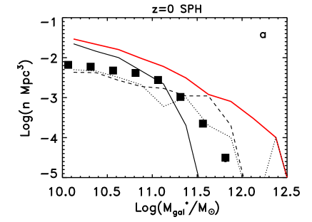
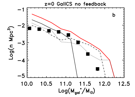
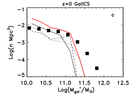
Figure 1: The galaxy mass functions computed with three different models (the SPH model, the no-feedback GalICS model, and the GalICS model with the feedback recipes of Section 3.4) compared with the observational estimate of Bell et al. (2003). In each of the three diagrams, the observational mass function is shown by the points and the theoretical one by the red line. The latter is decomposed into the mass functions of “field” galaxies (black solid line), “group” galaxies (dashed line) and “cluster” galaxies (dotted line), as described in the text.

4 Global view of the galaxy population

We consider three models: the SPH model, the GalICS model without any type of feedback, and the GalICS model with the feedback recipes described in Section 3.4. Because the feedback incorporated in the SPH simulation does not generally drive galactic winds or suppress gas cooling in massive haloes, it is the no-feedback GalICS model that is most comparable to the SPH simulation in its physical assumptions.

Figure 1 compares the galaxy baryonic mass functions at $z=0$ in these three models. (Here baryonic mass includes stars and the cold interstellar medium, but it does not include hot gas in the galaxy or group halo.) It also shows the separate contribution to the mass function of “field” galaxies ($M_{\rm halo}<3\times 10^{12}M_{\odot}$), “group” galaxies ($3\times 10^{12}M_{\odot}<M_{\rm halo}<10^{14}M_{\odot}$), and “cluster” galaxies ($M_{\rm halo}>10^{14}M_{\odot}$). In fact, the $34.19\,{\rm Mpc}$ simulation cube contains only a single “cluster” mass halo ($M=3\times 10^{14}M_{\odot}$), and the most massive “group” haloes are $\sim 3\times 10^{13}M_{\odot}$.

The SPH and no-feedback GalICS predictions agree remarkably well, both for the total baryonic mass function and for the separate mass functions in the three halo mass regimes. Feedback in the full GalICS model reduces galaxy masses, dropping the low mass end of the mass function and, most strikingly, producing sharp truncation of the high ends of the mass functions in the group and cluster haloes.

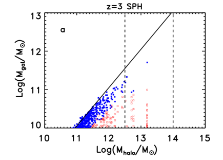
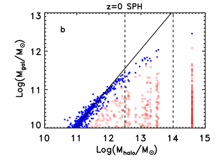
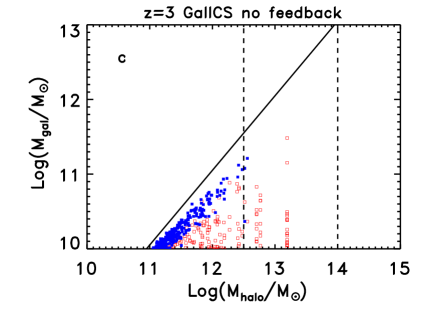
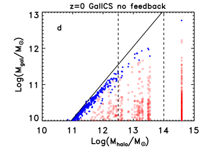
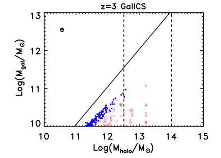
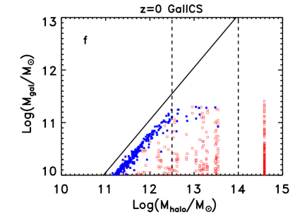
Figure 2: The galaxy content of dark matter haloes in the SPH simulation and in GalICS. The blue points correspond to galaxies that are at the centre of their dark matter halo, while the red points are satellite galaxies. In the SPH simulation, we always define the most massive galaxy to be “central.” In GalICS, a halo may have no central galaxy if it has had a recent merger, because dynamical friction takes time to make galaxies sink to the new centre of mass.

Points show the observational estimate of the total baryonic mass function from Bell et al. (2003), based on 2MASS and SDSS data. Because of the limited simulation volume, we would not expect perfect agreement with the data even for a model with exactly correct input physics. Nonetheless, the SPH and no-feedback GalICS predictions clearly exhibit the well known tendency of models with efficient gas cooling and minimal feedback to overproduce the baryonic mass function, a discrepancy that remains with larger simulation volumes (see Murali et al., 2002). The full GalICS model, by contrast, appears to underpredict the high mass end of the mass function. We believe that this is a real discrepancy, arising because the Hatton et al. (2003) feedback prescriptions are tuned to match the $B$-band luminosity function, and they produce massive galaxies that are too blue. The newer version of GalICS described by Cattaneo et al. (2006) shuts off gas accretion onto central galaxies of all high mass haloes and thereby achieves a simultaneous match to the $u$- and $r$-band luminosity functions.

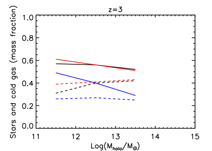
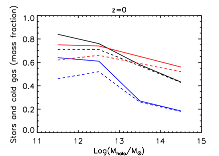
Figure 3: The fraction of the total baryonic content of a halo in stars (dashed lines) and in cold gas plus stars (solid lines) as a function of halo mass. The results of the SPH simulations are printed in black. The results of the GalICS model without feedback are printed in red. The results of the standard GalICS model are printed in blue.

Figure 4: The mass function of galaxies in the SPH simulation (points) and in the GalICS model (lines) at four different redshifts. In each panel, the dashed line is GalICS without supernova or AGN feedback, the solid line is the standard GalICS model, and the dotted line is the standard GalICS model when all masses are multiplied by a factor of 2.1. The mass function is given as the number of galaxies per logarithmic bin of 0.25 dex. In contrast to Fig. 1, we have not divided the number of galaxies by the volume of the computational box, so that the numbers convey an idea of the statistics in each bin. At $M_{\rm gal}>3\times 10^{11}M_{\odot}$, the number of galaxies in the box is $\mathrel{\hbox{\hbox to0.0pt{\hbox{\lower 4.0pt\hbox{$\sim$}}\hss}\hbox{$<$}}}10$, and statistical effects (quantified by the Poisson error bars) are no longer negligible.

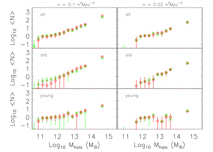
Figure 5: Mean halo occupations measured for the SPH galaxies (asterisks) and the full GalICS model galaxies (diamonds), at $z=0$. In the left (resp. right) panels, galaxies where selected in baryonic mass so as to yield a number density of $0.1h^{3}\,{\rm Mpc}^{-3}$ (resp. $0.02h^{3}\,{\rm Mpc}^{-3}$). From top to bottom, we show the mean occupation functions for the full, old, and young populations.

Figure 2 portrays the galaxy populations of all haloes in each of the three models, at $z=3$ and $z=0$. The “central” galaxy of each halo is marked by a blue point, while satellites in the same halo are marked by red points directly underneath. In GalICS, as in other semi-analytic models, central galaxies are treated specially — any cooling from the halo joins the central galaxy, not the satellites. The SPH simulation does not impose this physics a priori, but central galaxies nonetheless emerge as a distinct class. The galaxy closest to the halo centre-of-mass is almost always the most massive galaxy in the halo and it usually has the oldest stellar population (Berlind et al., 2003). Since the centre-of-mass is affected by asymmetries in the halo structure, the closest galaxy is occasionally a lower mass “satellite,” with the most massive galaxy nearby. For convenience, we have simply defined the most massive galaxy of each SPH halo to be the central galaxy. On closer inspection, this identification appears reasonable in virtually every case. While every SPH halo thus has a central galaxy by definition, a GalICS halo may not, if the halo has experienced a recent merger and there has not been sufficient time for dynamical friction to drag the most massive galaxy to the bottom of the halo potential well.

In all three models, the central galaxy baryonic mass is tightly correlated with halo mass, while satellite galaxy masses are broadly scattered with little correlation. Since most gas cooling in the SPH simulation and all gas cooling in the GalICS model occurs on the central galaxy, its growth is tightly coupled to the growth of the host halo. Most satellite galaxies, on the other hand, grew in smaller haloes, and they stopped growing after merging into a larger halo and becoming satellites.

At $M_{\rm halo}<3\times 10^{12}M_{\odot}$, both in the SPH model and in the GalICS model without feedback, most of the blue points are aligned very close to the $M_{\rm gal}=(\Omega_{\rm b}/\Omega_{\rm m})M_{\rm halo}$ black diagonal line, at least at $z=0$. That means that most of the halo baryons are in the central galaxy. At $M_{\rm halo}>3\times 10^{12}M_{\odot}$, this is less and less true for two reasons: a) in dense environments the cumulative baryonic content of satellite galaxies is more important, and b) as the cooling time of the hot gas becomes longer, a larger fraction of the baryons remain in the hot phase (Fig. 3). For these reasons, we take $M_{\rm halo}=3\times 10^{12}M_{\odot}$ as the border that separates field galaxies from group galaxies.

The addition of supernova and black hole feedback has two important effects. At low halo masses, ejection of gas by supernova feedback shifts the locus of central galaxy points down by about a factor of two, with concomitant reductions in satellite galaxy masses. The factor of two emerges because the ejected mass is, by construction, about equal to the mass that forms stars. This suppression is evident both at $z=3$ and at $z=0$. At $z=0$, black hole feedback has a much more drastic effect on massive galaxies, introducing a sharp cut-off at a total baryonic mass $\sim 3\times 10^{11}M_{\odot}$. The most massive galaxies in the no-feedback model are up to a factor of ten larger.

Figure 3 shows the mean mass of stars (dashed lines) and stars plus cold gas (solid lines) in bins of halo mass, now including central and satellite galaxy contributions. The SPH and no-feedback GalICS results agree fairly well at both $z=3$ and $z=0$, with GalICS predicting somewhat higher masses in the most massive $z=0$ haloes. The lower SPH stellar masses in low mass haloes are probably an artefact of limited numerical resolution, which leads to underestimated star formation rates and stellar masses in galaxies near the resolution threshold. We again see the factor of two reduction in baryonic masses due to feedback in the full GalICS model, which grows to a larger factor at high halo masses. Stellar masses are suppressed by about the same factor. Since the initial total gas content of each GalICS halo is $(\Omega_{b}/\Omega_{m})M_{\rm halo}$ by assumption, the baryons that are not in the cold gas plus stars phase are necessarily in the hot phase.

Figure 4 compares the galaxy baryonic mass functions at $z=3$, 1, 0.5, and 0. The generally good agreement between SPH and no-feedback GalICS seen in Figure 1 extends to higher redshifts. However, galaxy growth in no-feedback GalICS lags slightly (an effect also seen in Fig. 2), so its mass function begins somewhat lower at $z=3$ and catches up at low redshift. This difference may reflect the high efficiency of filamentary accretion (see Kereš et al., 2005) relative to the spherical accretion assumed in GalICS. The dotted lines in Figure 4 show the full GalICS mass function (solid line) after all galaxy masses are multiplied by a factor of 2.1. This shift brings it into good agreement with the SPH and no-feedback GalICS mass functions up to $M\sim 3\times 10^{11}M_{\odot}$, beyond which one sees the sharper cut-off induced by AGN feedback.

Figure 5 compares the halo occupation statistics of galaxies in the SPH simulation (asterisks) and the full GalICS model (diamonds), at $z=0$. In each model, we select galaxies above a baryonic mass threshold that yields a mean space density of $0.1h^{3}\,{\rm Mpc}^{-3}$ (left panels) or $0.02h^{3}\,{\rm Mpc}^{-3}$ (right panels). We have divided the galaxies in each panel into an old and a young population based on the median age of their stellar population. The old/young threshold was chosen in such way that the two subsets contain the same number of galaxies. Top, middle, and bottom panels show the mean occupation function (the average number of galaxies as a function of halo mass) for the full, old, and young populations, respectively.

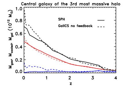
Figure 6: Growth history of the central galaxy of the third most massive halo ($M_{\rm halo}\sim 3\times 10^{13}M_{\odot}$) in the SPH simulation (solid lines) and in the GalICS model without feedback (dashed lines). The black lines show the total galaxy mass (stars plus cold galactic gas), while the red lines show mass of the gas that has cooled onto the galaxy since the beginning of the simulation. Galaxy mergers are the reason why the black lines are above the red lines. The blue lines show the cold galactic gas content in the SPH simulation and in the GalICS model without feedback.

The SPH and GalICS predictions agree impressively well, including the separate halo occupation statistics of old and young populations, which are quite different from each other. Berlind et al. (2003) found a similar level of agreement between a larger volume, lower resolution SPH simulation and the semi-analytic galaxy formation model of Cole et al. (2000). Although we do not show it here, the SPH and GalICS models exhibit comparably good agreement for the mean pair counts and triple counts ($\langle N(N-1)\rangle$ and $\langle N(N-1)(N-2)\rangle$) as a function of halo mass. The agreement of halo occupation statistics essentially guarantees that the SPH method and GalICS will make similar predictions for large scale clustering, even in larger volumes that are more statistically representative, and that this agreement will extend to the dependence of clustering on galaxy age and to the 3-point correlation statistics. On scales comparable to or smaller than the virial diameters of the largest haloes, the predicted spatial distribution of galaxies within haloes matters as well as the number of galaxies per halo. In investigating this issue, we found that the Hatton et al. (2003) prescription for computing satellite galaxy positions predicts spatial distributions in large haloes that are too diffuse, artificially suppressing small scale clustering (see Blaizot et al., 2006). However, a good agreement with the SPH simulation is achieved by simply associating satellite galaxies with randomly selected subsets of dark matter halo particles or dark matter sub-structures.

5 Galaxy growth

Galaxies grow by accreting gas and by merging with other galaxies. In this Section, we compare semi-analytic and SPH results at three different levels. First, we discuss the mass assembly of an individual galaxy (the central galaxy of the third most massive halo in the simulation at $z=0$). We do this by following the “main branch” of the galaxy tree, both in the SPH and in the GalICS outputs. That is, we recursively link the galaxy to its most massive progenitor. Second, we compare semi-analytic and SPH predictions for the total cooling rate integrated over this halo’s history. In the SPH simulation, we measure this quantity as the cumulative gas accretion rate of all the galaxy’s resolved progenitors at a given time. In GalICS, we simply add up the mass of the gas that cools in all the progenitors of our halo at each time-step. Notice that these two estimates are differently affected by resolution effects. In the semi-analytic case, we only consider cooling in haloes that contain more than 20 dark matter particles. In the SPH case, the limit is more vague, because cooling is not affected by resolution in a straightforward way. Hence the comparison is not precise, but it suffices for qualitative assessment. Third, we compare the total cooling rates in the entire simulation volume, for the SPH and the GalICS case. Here again, resolution affects the results slightly differently in the two methods.

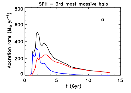
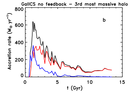
Figure 7: Gas accretion history of the galaxies in the third most massive halo contained in the computational box. The total amount of gas accreted by the galaxies in the halo at each cosmic time (black lines) has been decomposed into the contributions of the cold (blue) and the hot (red) mode. See Section 3.2 and Section 5 for an explanation of how we distinguish between “cold” and “hot” accretion.

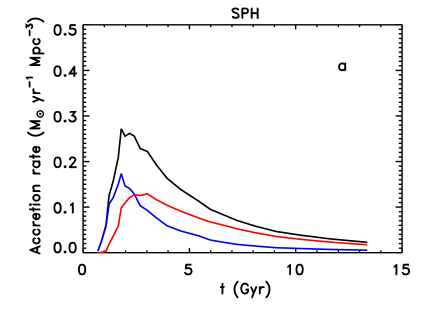
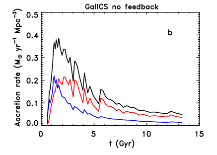
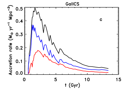
Figure 8: The rate at which galaxies accrete gas in a cosmic comoving volume. The total value (black lines) is decomposed into the contributions of the cold mode (blue lines) and the hot mode (red lines).

Figure 6 illustrates galaxy growth for the central object of the second most massive halo ($M_{\rm halo}\sim 3\times 10^{13}M_{\odot}$). We start from the galaxy at $z=0$ and trace it back in time by selecting the most massive progenitor at each step. The black solid line shows the growth of its total galaxy baryonic mass in the SPH simulation. The no-feedback GalICS model, shown by the black dashed line, is in very good agreement with the SPH model. The only notable differences are due to merging. In the SPH model there is a sudden increase of the galaxy mass from $5\times 10^{10}M_{\odot}$ to $1.3\times 10^{11}M_{\odot}$ at $z\sim 3.3-3.5$, produced by a major merger between two outputs. The semi-analytic model contains a similar merging event but it occurs slightly earlier (between the snapshot at $z\sim 3.7$ and the snapshot at $z\sim 3.5$) and the growth is somewhat smaller (from $4\times 10^{10}M_{\odot}$ to $8\times 10^{10}M_{\odot}$). The final difference in mass between the two galaxies is almost entirely due to a merger in the GalICS model at $z\sim 0.039-0.076$. In this merger, the twelfth since the first at $z\sim 3.5-3.7$, the galaxy mass has risen from $\sim 7.4\times 10^{11}M_{\odot}$ to $\sim 9.5\times 10^{11}M_{\odot}$. However, for the most part, the two growth curves nearly overlap.

The red solid and dashed lines show the total amount of gas accreted by the galaxy since the start of the simulation in the two calculations. In the absence of mergers, the red and the black lines of each type would coincide. From the agreement between the red solid and dashed lines, we see that the two methods agree on the relative amounts of accretion growth and merger growth. Finally, blue lines show the amount of cold gas in the galaxy as a function of redshift. The two methods agree well down to $z=1.5$. Below this redshift, the SPH simulation predicts a lower gas fraction, but the gas fraction is small in each case. The residual gas fraction in this gas-poor regime depends on the details of the star formation prescription, so some disagreement is expected.

Katz et al. (2003) and Kereš et al. (2005) have investigated gas accretion in the same SPH simulation that we are considering here. By tracing the temperature history of accreted particles, they have identified two distinct modes of gas accretion. About half of the gas follows the expected track in the conventional picture of galaxy formation: it shock-heats to the virial temperature of the galaxy’s potential well ($T\sim 10^{6}\,$K for a Milky Way type galaxy) before cooling, condensing, and forming stars. However, the other half radiates its acquired gravitational energy at much lower temperatures, typically $T<10^{5}\,$K. Cold accretion is often directed along filaments, allowing galaxies to draw gas efficiently from large distances, and it is dominant for low mass galaxies ($M_{\rm halo}<3\times 10^{11}M_{\odot}$). Hot accretion is quasi-spherical and dominates the growth of high mass systems.

Birnboim & Dekel (2003) and Dekel & Birnboim (2006) argue that the transition between the cold and hot accretion regimes is determined by the stability criterion for a shock at the halo’s viral radius, which in turn depends on the ratio of the post-shock cooling timescale to the dynamical time. Motivated by this argument, Croton et al. (2005) suggest that the cold and hot accretion regimes in hydrodynamic simulations should be identified with the rapid cooling and slow cooling regimes in semi-analytic models. We investigate this identification in Figures 7 and 8.

The black curve in Figure 7a shows the total accretion rate onto all galaxies in the third most massive halo of the SPH simulation as a function of time. The blue and the red curves show the cold and hot accretion rates, respectively. Here cold accretion consists of gas particles whose maximum temperature at any phase of their evolution is $T_{\rm max}<2.5\times 10^{5}\,$K. Because the $T_{\rm max}$ histogram is bimodal (Kereš et al., 2005), the division of hot and cold modes is insensitive to the exact choice of threshold. Figure 7b presents analogous results for the same halo in the no-feedback GalICS model. Here we identify cold accretion by the $r_{\rm cool}>r_{\rm infall}$ criterion discussed in Section 3.2. With this identification, the qualitative agreement between the SPH and GalICS calculations is quite good. In both cases there is a brief initial phase of cold accretion, when the universe is less than $\sim 2$ Gyr old, but hot accretion dominates after the halo becomes massive enough to support a virial shock. In the SPH simulation, cold and hot accretion can co-exist for the same galaxy (see Kereš et al., 2005), and in both calculations cold accretion continues onto lower mass galaxies that will subsequently join the main halo as satellites. However, the central galaxy of this halo is massive ($\sim 10^{12}M_{\odot}$) and contains a large fraction of the cooled baryons, so it dominates the accretion statistics. The cold accretion rate on galaxies in this halo is negligible at $t>5$ Gyr, in both calculations.

Figures 8a and 8b present a similar comparison for the accretion rates averaged over the entire simulation volume. The results are analogous, but cold accretion remains important for a longer time because most haloes are less massive than the one shown in Figure 7. The agreement between the SPH and the GalICS calculations is now even better.

Figure 8c shows the predictions of the full GalICS model with feedback. As discussed in Section 3.4, supernova feedback is modelled by assuming that supernovae drive a wind with an outflow rate approximately equal to the star formation rate, independent of the potential well’s depth. Since ejected gas may cool and be accreted again, perhaps multiple times, the total accretion rate in the full GalICS model is higher than that in Figures 8a or 8b, even though the final galaxy masses are lower. Gas entrained in a galactic wind is heated to the halo virial temperature, but if its subsequent cooling time is shorter than the infall time, we count it as cold accretion, just as we do for infalling gas. As most supernova feedback occurs in low mass galaxies with short cooling times, it is the cold accretion rate that rises significantly. Black hole feedback is modelled with a cooling cut-off in groups with $\Sigma M_{\rm bulge}>10^{11}M_{\odot}$, so it acts to suppress hot accretion in massive haloes. As a result, feedback reduces hot accretion in GalICS, especially at late times. The new GalICS model of Cattaneo et al. (2006) makes the assumption that all hot accretion is suppressed by AGN feedback, though it incorporates a more sophisticated calculation of where the cold-to-hot transition occurs.

6 The emergence of the galaxy bimodality

We now turn to our principal subject, the origin of bimodality in the galaxy population. We must first understand the connection between galaxy gas content and star formation rate (which we denote either by SFR or by $\dot{M_{*}}$). Figure 9 plots SFR against galaxy gas mass at $z=3$ and $z=0$, for the SPH, no-feedback GalICS, and full GalICS models. In each panel, red points represent satellite galaxies. Solid and dashed lines are the same in every panel and are provided for visual reference.

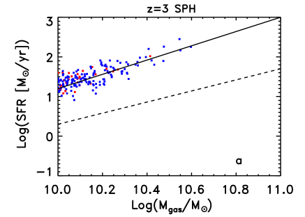
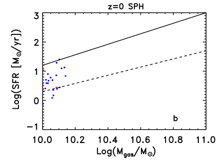
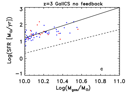
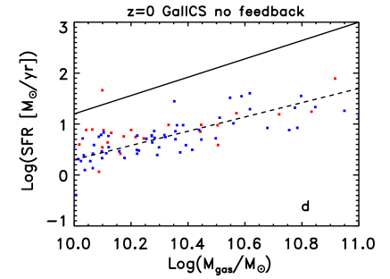
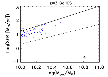
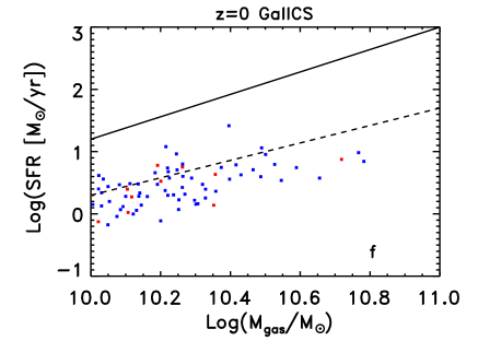
Figure 9: The relation between gas content and star formation rate in the SPH simulation (top), in the GalICS model without supernova or AGN feedback (centre) and in the standard GalICS model (bottom). The blue points correspond to galaxies that are at the centre of their dark matter halo (isolated field galaxies, brightest group or cluster galaxies), while the red points are satellite galaxies in groups or clusters. The solid line and the dashed line correspond to $1.8{\rm\,Log}M_{9}-0.6$ and $1.4{\rm\,Log}M_{9}-1.1$ , respectively ($M_{9}\equiv M_{\rm gas}/10^{9}M_{\odot}$). They are not fits and are just shown to guide the eye.

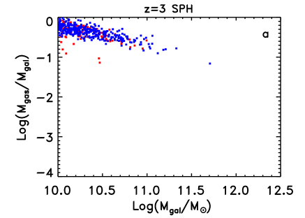
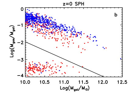
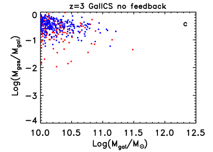
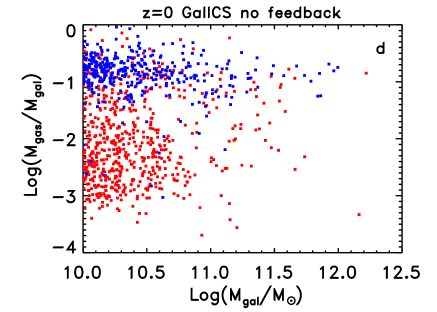
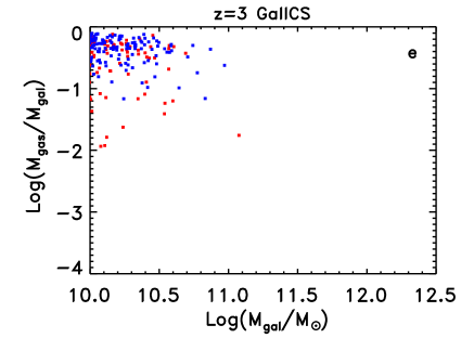
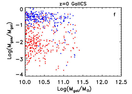
Figure 10: The gas fraction as a function of galaxy mass and redshift. The blue points correspond to galaxies that are at the centre of their dark matter halo, while the red points are satellite galaxies. The diagonal line in (b) shows the position of galaxy with a given mass and one gas SPH particle only. The galaxies below this line do not contain any measurable mass of gas. They have been attributed a gas mass drawn from a $10^{-3.5\pm 0.2}$ log-normal distribution for the gas fraction to put them on the plot.

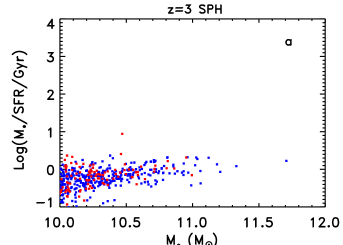
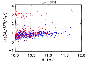
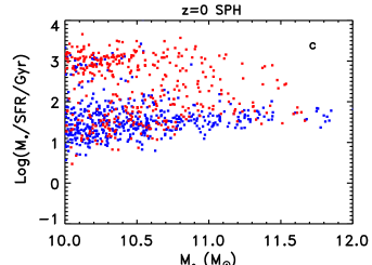
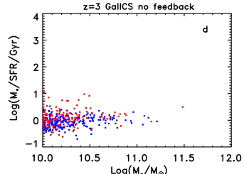
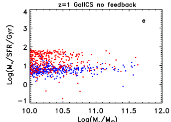
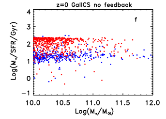
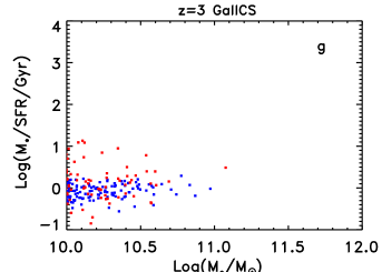
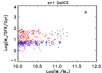
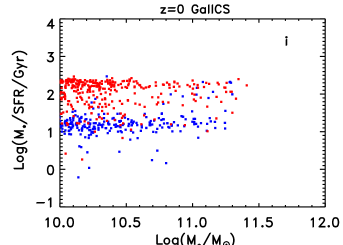
Figure 11: The relation between galaxy mass and $M_{*}/\dot{M}_{*}$ at different redshifts in the SPH simulation (top), in the GalICS model without supernova or AGN feedback (centre) and in the standard GalICS model (bottom). $M_{*}/\dot{M}_{*}$ is the time that a galaxy would have taken to form its stars if it had formed them at its current star formation rate. A value of $M_{*}/\dot{M}_{*}$ of the order of the Hubble time suggests a constant star formation rate throughout the life of the Universe. A value much longer than the Hubble time implies that the star formation rate has been much higher in the past than it is now and that the current star formation is negligible. The blue points are galaxies at the centre of their halo and the red points are satellite galaxies. SPH galaxies with zero SFR have been displayed on the plot by attributing them a value of ${\rm Log}(M_{*}/\dot{M}_{*}/{\rm Gyr})$ drawn from a $3\pm 0.2$ Gaussian distribution.

At $z=3$, the SPH and no-feedback GalICS populations show similar trends between gas mass and SFR, roughly SFR$=16(M_{\rm gas}/10^{10}M_{\odot})^{1.8}M_{\odot}\,{\rm yr}^{-1}$. There is substantial scatter about the mean relation but no obvious difference between central and satellite galaxies of the same gas mass. The SFR at fixed gas mass in the full GalICS model is lower by a factor $\sim 2$, but the slope of the trend is similar. At $z=0$, the SFR for a given $M_{\rm gas}$ is lower than at $z=3$, as expected given the characteristically larger sizes and lower surface densities of low redshift galaxies. The SFRs are slightly higher at fixed $M_{\rm gas}$ in the SPH simulation, but there are many fewer galaxies with large gas masses because massive galaxies in the SPH simulation convert nearly all of their gas into stars. The trends in Figure 9 are determined largely by the star formation law, which is qualitatively similar among the three models (even though the feedback prescriptions are different).

Figure 10 plots gas fraction against galaxy baryonic mass. Here we see important differences among the three models and the first indications of bimodal galaxy populations. As in Figure 9, blue points represent central galaxies and red points satellite galaxies. At $z=0$, the no-feedback GalICS model shows two distinct, albeit fuzzy sequences in this $M_{\rm gas}/M_{\rm gal}$ vs. $M_{\rm gal}$ plane. The gas rich sequence is centred on $M_{\rm gas}/M_{\rm gal}\sim 0.2$, while the gas poor sequence is centred on $M_{\rm gas}/M_{\rm gal}\sim 0.005$, with a large scatter. Most central galaxies occupy the gas rich sequence and most satellite galaxies occupy the gas poor sequence, but there are exceptions in both directions. The most obvious effect of feedback in the full GalICS model is to reduce the baryonic masses of the most massive galaxies, to a maximum of $\sim 3\times 10^{11}M_{\odot}$. In contrast to the no-feedback GalICS case, many of the most massive central galaxies are gas poor instead of gas rich.

In the SPH simulation, it is possible for a galaxy to have a gas fraction of zero, if all of the particles that compose it are purely stellar. We have arbitrarily assigned these galaxies a gas fraction of $10^{-3.5}$ with a 0.2 dex scatter, so that one can see them in Figure 10b. The dashed line in this panel shows the gas fraction for a galaxy that contains one gas SPH particle only. There is a significant gap between the bottom edge of the upper sequence of points and this discreteness limit. This gap suggests a genuinely bimodal behaviour rather than an artificially divided continuum, with all points above the line belonging to the gas rich sequence. Within this sequence, satellite galaxies have lower average gas fractions than central galaxies of the same mass. There is also a trend of decreasing gas fraction with increasing galaxy mass, but this is at least partly an artefact of resolution: gas densities are underestimated in low mass galaxies, and gas consumption by star formation is thus underestimated as well. Consequently, we do not regard this trend as a robust prediction, at least for masses below $M_{\rm gal}\sim 2\times 10^{10}M_{\odot}$ (less than about 200 SPH particles). Once we account for the resolution and discreteness effects, the SPH results appear qualitatively similar to the no-feedback GalICS results, with the notable exception that many SPH satellites occupy the low end of the gas rich sequence rather than the separate gas poor sequence.

Figure 11 presents the principal result of this paper, the distribution of galaxies in the plane of stellar mass and star formation time-scale, $M_{*}/\dot{M}_{*}$. Dividing the Hubble time $t_{0}=13.4\,$Gyr by this time-scale gives the ratio of the galaxy’s current SFR to its time-averaged SFR. The light from galaxies with long star formation time-scales is dominated by red giants from old stellar populations, while young stars produce a significant amount of blue light in galaxies with more current star formation. Figure 11 is thus a theoretical version of a galaxy “colour-magnitude” diagram. At low redshift, many SPH galaxies have zero star formation rate. We have arbitrarily assigned these galaxies time-scales of $10^{3}$ Gyr, with random scatter of 0.2 dex, so that they appear on these plots. The GalICS time-scale distributions have a sharp upper edge at $M_{*}/\dot{M}_{*}\sim 10^{2.4}\,$Gyr. To understand its origin, consider the specific SFR, $\dot{M}_{*}/M_{*}=(\dot{M}_{*}/M_{\rm gas})/(M_{\rm gas}/M_{*})$. The first term is $\dot{M}_{*}/M_{\rm gas}\sim 2(M_{\rm gas}/10^{10}M_{\odot})^{0.4}M_{\odot}{\rm yr}^{-1}$ (Figure 9). The second term is $M_{\rm gas}/M_{*}\mathrel{\hbox{\hbox to0.0pt{\hbox{\lower 4.0pt\hbox{$\sim$}}\hss}\hbox{$>$}}}10^{-3}$ in the GalICS model, but not in the SPH model, where many galaxies contain no gas at all (Figure 10). The tendency of GalICS galaxies to retain a minimum gas fraction explains the upper edge in the $M_{*}/\dot{M}_{*}$ distribution.

The main features of Figure 11 follow naturally from the trends in Figures 9 and 10. At $z=0$, the SPH simulation has a bimodal galaxy distribution. The old (red) sequence is populated mainly by satellite galaxies, with a few lower mass central galaxies mixed in. The young (blue) sequence contains a mix of central and satellite galaxies, but the consumption of gas in satellites is evidently fast enough to leave few galaxies with intermediate star formation time-scales. The most massive central galaxies all reside on the young sequence because of their continuing gas accretion, as seen already in Figure 10. Results for the no-feedback GalICS model are similar, except that there are fewer satellites in the young sequence. In GalICS, galaxies experience no gas accretion at all once they fall into larger haloes and become satellites. In the SPH simulation, some satellites continue to accrete gas, e.g. because they are the central objects of sub-haloes that have not yet dissolved and lost their identity. The complete shutoff of accretion in GalICS satellites therefore appears overly drastic.

Results for the full GalICS model are similar, with the crucial distinction that many of the massive central galaxies are now on the old sequence. As we have already emphasised, this observational success of the full GalICS model is a consequence of AGN feedback, which suppresses continuing gas accretion in the most massive haloes. The SPH and no-feedback GalICS populations do include some fairly massive galaxies in the old sequence, but nearly all of these are satellites in the most massive halo (see Figure 2). This halo is anomalously large for this simulation volume, so a larger simulation would probably yield a smaller fraction of massive old galaxies in these two models.

Kauffmann et al. (2004) have investigated the distribution of $\dot{M}_{*}/M_{*}$ in the SDSS, using spectral line diagnostics to estimate star formation rates and stellar mass-to-light ratios. They obtain a bimodal distribution with peaks corresponding to $\log(M_{*}/\dot{M}_{*}/{\rm Gyr})\sim 1.2$ and 2.6, in reasonable agreement with the GalICS predictions in Figure 11. The typical star formation time-scales on the young sequence in the SPH simulation appear slightly too long.

Moving to higher redshift, we see that all three models predict a unimodal distribution of star formation time-scales at $z=3$, with typical value $M_{*}/\dot{M}_{*}\sim 1\,$Gyr. By $z=1$, the time-scale on the young sequence has increased to about $4\,$Gyr, and an old sequence has begun to emerge. In the SPH and no-feedback GalICS populations, this sequence mostly contains relatively low mass satellites. However, in the full GalICS model the central galaxies of the most massive $z=1$ haloes have already joined the “red and dead” population.

7 Summary and Discussion

We have compared the galaxy populations of an SPH simulation, the hybrid GalICS model of Hatton et al. (2003), and a stripped down version of this model with no feedback from star formation or AGN. The GalICS calculations are applied to the dark matter halo population extracted from the SPH simulation, allowing direct comparison of the results.

For the most part, the SPH and no-feedback GalICS predictions agree remarkably well. In particular, the two methods predict similar galaxy baryonic mass functions and similar dependence of these mass functions on environment and redshift. The SPH simulation predicts somewhat more rapid growth at high redshift, probably a consequence of efficient filamentary accretion and a star formation time-scale that tracks the shorter dynamical time-scales of high redshift galaxies. The global gas accretion histories are similar in the two calculations, and this agreement extends to the individual galaxy level as shown in Figure 6. The breakdown between cold and hot accretion in the SPH simulation is qualitatively similar to the breakdown between the rapid cooling ($r_{\rm cool}>r_{\rm infall}$) and slow cooling ($r_{\rm cool}<r_{\rm infall}$) accretion in GalICS. This agreement supports the suggestion by Croton et al. (2005) that the cold/hot dichotomy seen in hydrodynamic simulations (Katz, 1992; Katz et al., 2003; Birnboim & Dekel, 2003; Kereš et al., 2005; Dekel & Birnboim, 2006) can be identified with the infall-dominated/cooling-dominated regimes of traditional semi-analytic models (White & Frenk, 1991; Kauffmann et al., 1993; Cole et al., 1994). Kereš et al. (2005) note some important caveats to this identification, especially for models that incorporate a photoionising background, which increases cooling time-scales in low mass haloes.

Both the SPH and the no-feedback GalICS models predict a bimodal galaxy population with a “blue” sequence of gas-rich, star-forming galaxies and a “red” sequence of gas-poor galaxies dominated by old stellar populations. The red sequence is populated mainly by satellite galaxies, which stop accreting gas after they fall into larger haloes. A larger fraction of SPH satellites remain on the gas rich, star-forming sequence, which suggests that the truncation of gas accretion in GalICS is unrealistically abrupt. However, both calculations agree on a crucial point: the central galaxies of massive haloes experience continuing gas accretion, and they therefore remain on the star-forming sequence. The masses of these galaxies are substantially larger than those inferred for galaxies of similar space density in the real universe — i.e., both models drastically overpredict the high end of the galaxy baryonic mass function. There is also agreement that gas accretion by satellites in cluster-size haloes is negligible.

While the agreement between SPH and no-feedback GalICS could in principle reflect a conspiracy of errors, it seems more reasonable to conclude that both methods do a fairly accurate job of modelling the growth of galaxies from cosmological initial conditions. This conclusion in turn implies that the observational failings of these models are a consequence of missing input physics. The full GalICS model is much more successful in reproducing observations because of its prescriptions for supernova and AGN feedback. Supernova feedback reduces the masses of low and intermediate mass galaxies by about a factor of two, as the gas outflow rate is comparable to the star formation rate by construction. AGN feedback produces a sharp cut-off in the baryonic mass function by suppressing the cooling of gas in high mass haloes. Crucially, this mechanism also moves the central galaxies of massive haloes to the old, gas-poor sequence.

Some mechanism that suppresses gas cooling in massive haloes appears essential to explaining both the exponential cut-off in the observed galaxy luminosity function (Kauffmann et al., 1993; Benson et al., 2003) and the observed form of bimodality in the galaxy population, where nearly all of the most massive galaxies reside on the red sequence (Blanton et al., 2003; Kauffmann, 2003). As argued by Birnboim & Dekel (2003), Katz et al. (2003), Binney (2004), Kereš et al. (2005), and Dekel & Birnboim (2006), it seems natural to associate this mechanism with the “hot mode” of gas accretion that becomes dominant in haloes more massive than $\sim 10^{12}M_{\odot}$, since the implied mass scale is close to the transition mass inferred observationally by Kauffmann (2003) and since the amounts of cool gas in observed galaxy clusters are much lower than predicted by the X-ray cooling rates in the absence of heating (e.g., Kaastra et al., 2001). In this view, the factor that determines the effectiveness of AGN feedback is not so much the mass of the black hole as the state of the gas that it will affect. Even a luminous AGN will have difficulty reversing the inflow of dense, cold gas along filamentary streams, or ejecting the interstellar medium of a galaxy disc. However, an AGN can couple more easily to the diffuse, quasi-spherical hot atmosphere of a massive halo, and, with plausible accretion rates and efficiencies, there is enough energy to suppress the gas cooling that would otherwise be expected in these haloes (see, e.g., Best et al., 2006).

In this regard, it is interesting that the new GalICS model of Cattaneo et al. (2006) is considerably more successful than the Hatton et al. (2003) version of GalICS tested here. The Hatton et al. implementation ties AGN feedback to black hole mass and, thus, to bulge mass. This prescription suppresses cooling in massive haloes, but not effectively enough. Massive galaxies do lie on a “red” sequence separated from the “blue” sequence of star-forming galaxies. Nevertheless, a quantitative comparison with the observations obtained using a stellar population synthesis model shows that they are still not red enough. Strong supernova feedback, achieved by assuming that the mass loss rate through a supernova-driven wind is approximately equal to the star formation rate independently of the depth of the potential well, can compensate the incomplete shutdown of cooling in massive haloes, but it also ejects too many metals. The Cattaneo et al. (2006) model completely suppresses gas accretion in haloes above the critical mass where virial shocks arise, computed via the methods of Dekel & Birnboim (2006). This implementation yields excellent agreement with the observed colour-luminosity distribution of galaxies at low and high redshift.

Croton et al. (2005) achieve a similar level of observational success in a hybrid model that uses kinetic feedback from radio-loud AGN to suppress gas cooling in massive haloes. Because this mechanism is assumed to affect only the quasi-hydrostatic atmospheres that arise in haloes with long post-shock cooling times, the practical effect of this scheme is quite similar to the sharp cut-off in the Cattaneo et al. (2006) model. Very recently, Bower et al. (2006) have presented another model that is very similar to that of Cattaneo et al. (2006), both in the method and the key results.

There is still much to be understood about the physics that suppresses gas cooling in massive haloes, i.e., the detailed mechanism by which AGN energy couples to the surrounding gas, or even whether AGN are really the source of this suppression at all. However, it is striking that the theoretically derived mass scale separating the cold and hot accretion regimes corresponds so well to the observed mass scale that marks the transition between the blue and red galaxy populations, and that the most successful models of the observed galaxy population are those that incorporate suppressed hot accretion to identify one transition with the other.

8 Acknowledgements

We acknowledge stimulating discussions with A. Dekel. A.C. has been supported by a Marie Curie Research Fellowship at the IAP and by a Golda Meir Fellowship at the Hebrew University of Jerusalem. Additional support for this research has come from NASA Grant NAGS-13308. D.W. thanks the IAP for hospitality during the initial stages of this work.

References

- Baldry et al. (2004) Baldry I. K., Glazebrook K., Brinkmann J., Ivezić Ž., Lupton R. H., Nichol R. C., Szalay A. S., 2004, ApJ, 600, 681
- Balogh et al. (2004) Balogh M. L., Baldry I. K., Nichol R., Miller C., Bower R., Glazebrook K., 2004, ApJL, 615, L101
- Barnes & Hut (1986) Barnes J., Hut P., 1986, Nature, 324, 446
- Bell et al. (2003) Bell E. F., McIntosh D. H., Katz N., Weinberg M. D., 2003, ApJS, 149, 289
- Bell et al. (2004) Bell E. F., Wolf C., Meisenheimer K., Rix H.-W., Borch A., Dye S., Kleinheinrich M., Wisotzki L., McIntosh D. H., 2004, ApJ, 608, 752
- Benson et al. (2003) Benson A. J., Bower R. G., Frenk C. S., Lacey C. G., Baugh C. M., Cole S., 2003, ApJ, 599, 38
- Benson et al. (2001) Benson A. J., Pearce F. R., Frenk C. S., Baugh C. M., Jenkins A., 2001, MNRAS, 320, 261
- Berlind et al. (2003) Berlind A. A., Weinberg D. H., Benson A. J., Baugh C. M., Cole S., Davé R., Frenk C. S., Jenkins A., Katz N., Lacey C. G., 2003, ApJ, 593, 1
- Best et al. (2006) Best P. N., Kaiser C. R., Heckman T. M., Kauffmann G., 2006, pre-print astro-ph/0602171
- Binney (2004) Binney J., 2004, MNRAS, 347, 1093
- Birnboim & Dekel (2003) Birnboim Y., Dekel A., 2003, MNRAS, 345, 349
- Blaizot et al. (2004) Blaizot J., Guiderdoni B., Devriendt J. E. G., Bouchet F. R., Hatton S. J., Stoehr F., 2004, MNRAS, 352, 571
- Blaizot et al. (2006) Blaizot J., Szapudi I., Colombi S., Budavari T., Bouchet F. R., Devriendt J. E. G., Guiderdoni B., Pan J., Szalay A., 2006, pre-print astro-ph/0603821
- Blanton et al. (2005) Blanton M. R., Eisenstein D., Hogg D. W., Schlegel D. J., Brinkmann J., 2005, ApJ, 629, 143
- Blanton et al. (2003) Blanton M. R., Hogg D. W., Bahcall N. A., Baldry I. K., Brinkmann J., Csabai I., Eisenstein D., Fukugita M., Gunn J. E., Ivezić Ž., 2003, ApJ, 594, 186
- Bower et al. (2006) Bower R. G., Benson A. J., Malbon R., Helly J. C., Frenk C. S., Baugh C. M., Cole S., Lacey C. G., 2006, pre-print astro-ph/0511338
- Cattaneo et al. (2005) Cattaneo A., Blaizot J., Devriendt J., Guiderdoni B., 2005, MNRAS, 364, 407
- Cattaneo et al. (2006) Cattaneo A., Dekel A., Devriendt J., Guiderdoni B., Blaizot J., 2006, pre-print astro-ph/0601295
- Cole et al. (1994) Cole S., Fisher K. B., Weinberg D. H., 1994, MNRAS, 267, 785
- Cole et al. (2000) Cole S., Lacey C. G., Baugh C. M., Frenk C. S., 2000, MNRAS, 319, 168
- Croton et al. (2005) Croton D. J., Springel V., White S. D. M., De Lucia G., Frenk C. S., Gao L., Jenkins A., Kauffmann G., Navarro J. F., Yoshida N., 2005, MNRAS, p. 1055
- Dave et al. (1997) Dave R., Dubinski J., Hernquist L., 1997, New Astronomy, 2, 277
- Davé et al. (1999) Davé R., Hernquist L., Katz N., Weinberg D. H., 1999, ApJ, 511, 521
- Davis et al. (1985) Davis M., Efstathiou G., Frenk C. S., White S. D. M., 1985, ApJ, 292, 371
- De Lucia et al. (2004) De Lucia G., Kauffmann G., White S. D. M., 2004, MNRAS, 349, 1101
- Dekel & Birnboim (2006) Dekel A., Birnboim Y., 2006, pre-print astro-ph/0412300
- Evrard et al. (1994) Evrard A. E., Summers F. J., Davis M., 1994, ApJ, 422, 11
- Faber et al. (2005) Faber S. M., Willmer C. N. A., Wolf C., Koo D. C., Weiner B. J., Newman J. A., Im M., Coil A. L., Conroy C., Cooper M. C., Davis M., Finkbeiner D. P., 2005, pre-print astro-ph/0506044
- Frenk et al. (1999) Frenk C. S., White S. D. M., Bode P., Bond J. R., Bryan G. L., Cen R., Couchman H. M. P., Evrard 1999, ApJ, 525, 554
- Gelb & Bertschinger (1994) Gelb J. M., Bertschinger E., 1994, ApJ, 436, 467
- Gingold & Monaghan (1977) Gingold R. A., Monaghan J. J., 1977, MNRAS, 181, 375
- Guiderdoni et al. (1998) Guiderdoni B., Hivon E., Bouchet F. R., Maffei B., 1998, MNRAS, 295, 877
- Haardt & Madau (1996) Haardt F., Madau P., 1996, ApJ, 461, 20
- Hatton et al. (2003) Hatton S., Devriendt J. E. G., Ninin S., Bouchet F. R., Guiderdoni B., Vibert D., 2003, MNRAS, 343, 75
- Helly et al. (2003) Helly J. C., Cole S., Frenk C. S., Baugh C. M., Benson A., Lacey C., Pearce F. R., 2003, MNRAS, 338, 913
- Hernquist (1987) Hernquist L., 1987, ApJS, 64, 715
- Hernquist & Katz (1989) Hernquist L., Katz N., 1989, ApJS, 70, 419
- Hogg et al. (2004) Hogg D. W., Blanton M. R., Brinchmann J., Eisenstein D. J., Schlegel D. J., Gunn J. E., McKay T. A., Rix H., Bahcall N. A., Brinkmann J., Meiksin A., 2004, ApJL, 601, L29
- Hubble (1926) Hubble E. P., 1926, ApJ, 64, 321
- Humason (1936) Humason M. L., 1936, ApJ, 83, 10
- Kaastra et al. (2001) Kaastra J. S., Ferrigno C., Tamura T., Paerels F. B. S., Peterson J. R., Mittaz J. P. D., 2001, A&A, 365, L99
- Katz (1992) Katz N., 1992, ApJ, 391, 502
- Katz et al. (2003) Katz N., Keres D., Dave R., Weinberg D. H., 2003, in Rosenberg J. L., Putman M. E., eds, ASSL Vol. 281: The IGM/Galaxy Connection. The Distribution of Baryons at z=0 How Do Galaxies Get Their Gas?. p. 185
- Katz et al. (1996) Katz N., Weinberg D. H., Hernquist L., 1996, ApJS, 105, 19
- Kauffmann et al. (1999) Kauffmann G., Colberg J. M., Diaferio A., White S. D. M., 1999, MNRAS, 303, 188
- Kauffmann et al. (2003) Kauffmann G., Heckman T. M., White S. D. M., Charlot S., Tremonti C., Peng E. W., Seibert M., Brinkmann J., Nichol R. C., SubbaRao M., York D., 2003, MNRAS, 341, 54
- Kauffmann et al. (1993) Kauffmann G., White S. D. M., Guiderdoni B., 1993, MNRAS, 264, 201
- Kauffmann et al. (2004) Kauffmann G., White S. D. M., Heckman T. M., Ménard B., Brinchmann J., Charlot S., Tremonti C., Brinkmann J., 2004, MNRAS, 353, 713
- Kauffmann (2003) Kauffmann G. e., 2003, MNRAS, 341, 33
- Kennicutt (1998) Kennicutt R. C., 1998, ApJ, 498, 541
- Kereš et al. (2005) Kereš D., Katz N., Weinberg D. H., Davé R., 2005, MNRAS, 363, 2
- Lanzoni et al. (2005) Lanzoni B., Guiderdoni B., Mamon G. A., Devriendt J., Hatton S., 2005, MNRAS, 361, 369
- Lucy (1977) Lucy L. B., 1977, AJ, 82, 1013
- Miller & Scalo (1979) Miller G. E., Scalo J. M., 1979, ApJS, 41, 513
- Murali et al. (2002) Murali C., Katz N., Hernquist L., Weinberg D. H., Davé R., 2002, ApJ, 571, 1
- Pearce et al. (2001) Pearce F. R., Jenkins A., Frenk C. S., White S. D. M., Thomas P. A., Couchman H. M. P., Peacock J. A., Efstathiou G., 2001, MNRAS, 326, 649
- Quinn et al. (1996) Quinn T., Katz N., Efstathiou G., 1996, MNRAS, 278, L49
- Sánchez et al. (2006) Sánchez A. G., Baugh C. M., Percival W. J., Peacock J. A., Padilla N. D., Cole S., Frenk C. S., Norberg P., 2006, MNRAS, 366, 189
- Schechter (1976) Schechter P., 1976, ApJ, 203, 297
- Schmidt (1959) Schmidt M., 1959, ApJ, 129, 243
- Silk (2001) Silk J., 2001, MNRAS, 324, 313
- Silk (2003) Silk J., 2003, MNRAS, 343, 249
- Spergel et al. (2003) Spergel D. N., Verde L., Peiris H. V., Komatsu E., Nolta M. R., Bennett C. L., Halpern M., Hinshaw G., Jarosik N., Kogut A., Limon M., Meyer S. S., Page L., Tucker G. S., Weiland J. L., Wollack E., Wright E. L., 2003, ApJS, 148, 175
- Springel et al. (2001) Springel V., Yoshida N., White S. D. M., 2001, New Astronomy, 6, 79
- Stinson et al. (2006) Stinson G., Seth A., Katz N., Wadsley J., Governato F., Quinn T., 2006, pre-print astro-ph/0602350
- Strateva et al. (2001) Strateva I., Ivezić Ž., Knapp G. R., Narayanan V. K., Strauss M. A., Gunn J. E., Lupton R. H., Schlegel D., Bahcall N. A., 2001, AJ, 122, 1861
- Sutherland & Dopita (1993) Sutherland R. S., Dopita M. A., 1993, ApJS, 88, 253
- Tegmark et al. (2004) Tegmark M., Strauss M. A., Blanton M. R., Abazajian K., Dodelson S., Sandvik H., Wang X., Weinberg D. H., Zehavi I., Bahcall N. A., 2004, Phys. Rev. D, 69, 103501
- Thoul & Weinberg (1996) Thoul A. A., Weinberg D. H., 1996, ApJ, 465, 608
- van Dokkum et al. (2006) van Dokkum P. G., Quadri R., Marchesini D., Rudnick G., Franx M., Gawiser E., Herrera D., Wuyts S., Lira P., Labbé I., Maza J., 2006, ApJL, 638, L59
- White & Frenk (1991) White S. D. M., Frenk C. S., 1991, ApJ, 379, 52
- Yoshida et al. (2002) Yoshida N., Stoehr F., Springel V., White S. D. M., 2002, MNRAS, 335, 762