The CFHTLS Real Time Analysis System:
”Optically Selected GRB Afterglows”

Abstract

Aims. We describe a deep and wide search for optical GRB afterglows in images taken with MegaCAM at the Canada France Hawaii Telescope, within the framework of the CFHT Legacy Survey.

Methods. This search is performed in near real-time thanks to a Real Time Analysis System (RTAS) called ”Optically Selected GRB Afterglows”, which has been installed on a dedicated computer in Hawaii. This pipeline automatically and quickly analyzes Megacam images to construct catalogs of astronomical objects, and compares catalogs made from images taken at different epochs to produce a list of astrometrically and photometrically variable objects. These objects are then displayed on a web page to be characterized by a member of the collaboration.

Results. In this paper, we comprehensively describe the RTAS process from image acquisition to the final characterization of variable sources. We present statistical results based on one full year of operation, showing the quality of the images and the performance of the RTAS. The limiting magnitude of our search is r’=22.5 on average and the observed area amounts to 1178 square degrees. We have detected about 13.10⁶ astronomical sources of which about 0.01% are found to vary by more than one tenth of a magnitude. We discuss the performance of our instrumental setup with a sample of simulated afterglows. This sample allows us to compare the efficiency of our search with previous works, to propose an optimal observational strategy, and to discuss general considerations on the searches for GRB optical afterglows. We postpone to a forthcoming paper the discussion of the characterization of variable objects we have found, and a more detailled analysis of the nature of those resembling GRB afterglows.

Conclusions. The RTAS has been continuously operating since November 2004. Each month 15-30 square degrees are observed many times over a period of 2-3 nights. The real-time analysis of the data has revealed no convincing afterglow candidate so far.

1 Introduction

Long gamma-ray bursts (hereafter GRBs) are cosmological events due to powerful stellar explosions in distant galaxies. They are composed of two phases: the prompt emission, a short and bright flash of $\gamma$-ray and X-ray photons, and the afterglow, a fainter decaying emission visible from X-ray to radio wavelengths. Current observations of the prompt GRB emission and of the afterglow are satisfactorily described in the framework of the internal-external shock model. This model explains the prompt emission as the radiation emitted by internal shocks within an unsteady outflow of ultra-relativistic material (Rees & Mészáros rees94 (1994)), and the afterglow by the shock of the ultra-relativistic outflow on the medium surrounding the source (e.g. Rees & Mészáros rees92 (1992), Mészáros & Rees meszaros97 (1997), Wijers et al. wijers97 (1997)). Based on theoretical and observational grounds, there is now a general consensus on the fact that the prompt GRB emission is collimated into a jet which broadens gradually as its bulk Lorentz factor decreases.

One strong argument in favor of GRB collimation is that it greatly reduces the energy requirements at the source. For example an event like GRB 990123 would have released of the order of 3 10⁵⁴ erg of high-energy radiation if it were radiating isotropically (Kulkarni et al. kulkarni99 (1999)). This energy budget can be reduced to 2 10⁵¹ erg if we assume that the prompt $\gamma$-ray emission was collimated into two opposite jets with a FWHM of 2.9^∘ (e.g. Frail et al. frail01 (2001)). Theoretical calculations of the evolution of the ejecta have shown that the afterglows of beamed gamma-ray bursts must exhibit an achromatic ’jet break’ when $1/\Gamma$, the inverse of the bulk Lorentz factor of the jet, becomes comparable to $\theta$, the opening angle of the jet (Rhoads rhoads97 (1997)). From the observational point of view, the light-curves of several GRB afterglows display achromatic breaks, observed at optical and X-ray wavelengths, hours to days after the burst (e.g. Harrison et al. harrison99 (1999)), providing strong observational evidence in favor of GRB beaming. Interpreting these breaks as signatures of the beaming of the high-energy emission gives opening angles ranging from 3° to 30°. Even if the signature of GRB jets in the light-curves of the afterglows remains a subject of debate (see for instance Wei & Lu wei00 (2000), Moderski et al. moderski00 (2000)) and if other causes can produce breaks in GRB afterglow light-curves (e.g. cooling breaks, Sari sari98 (1998)), the jet break interpretation is supported by the intriguing fact that the energy output corrected from beaming appears well clustered around 10⁵¹ erg, with a dispersion much smaller than the energy output obtained assuming isotropic emission (Frail et al. frail01 (2001), Panaitescu & Kumar panaitescu01 (2001), Bloom, Frail & Kulkarni bloom03 (2003)). This result can be interpreted as the evidence that GRBs have a standard energy reservoir (Frail et al. frail01 (2001), Panaitescu & Kumar panaitescu01 (2001), Piran et al. piran01 (2001)), or as the evidence that GRB jets have a universal configuration (Zhang & Mészáros zhang02 (2002)).

One remarkable prediction of the models of jetted GRBs is that the jet starts to spread out when the afterglow is still detectable, allowing the afterglow to become visible for off-axis observers. This prediction has led to the concept of ’orphan afterglows’, initially used for the afterglows of off-axis GRBs. Afterglows of off-axis GRBs have been studied from a theoretical point of view by many authors (Rhoads rhoads97 (1997), Rhoads rhoads99 (1999), Wei & Lu wei00 (2000), Totani & Panaitescu totani02 (2002), Nakar et al. nakar02 (2002), Dalal et al. dalal02 (2002)). Recently, it has been realized that orphan afterglows could be also produced by failed on-axis GRBs, which are fireballs with Lorentz factors well below 100 but larger than a few (Huang et al. huang02 (2002)).

This short discussion illustrates the reasons that make the existence of orphan afterglows quite probable (both from off-axis GRBs and from failed GRBs), and their relation with GRBs non-trivial (e.g. Dalal et al. dalal02 (2002), Huang et al. huang02 (2002)). Given the potential pay-off which would result from the detection of even a few orphan afterglows (energetics, distance, rate of occurrence…), it is important trying detecting them. As explained above, the detection of orphan GRB afterglows offers a complementary way to test the beaming hypothesis and can constrain the beaming factor. Additionally, since afterglows of off-axis GRBs are expected to be more numerous but fainter, they will be detectable at lower redshifts. Their detection could thus help estimating the local population of faint GRBs ($z<<0.1$), of which GRB980425 (z=0.0085) and GRB060218 (z=0.033) are the best known examples.

In short, we are motivated by the fact that the detection of orphan afterglows may open a completely new way to detect GRBs and permit the study of a population of GRBs which is not or very poorly studied at present (all GRBs known to date having been detected by their high-energy emission). The motivations driving the searches for GRB orphan afterglows have been discussed by various authors like Totani & Panaitescu (totani02 (2002)), Nakar & Piran (nakar02 (2002)), Kehoe et al. (kehoe02 (2002)), Groot et al. (groot03 (2003)), Rykoff et al. (rykoff05 (2005)) in the optical range, by Greiner et al. (greiner99 (1999)) for X-ray afterglows, and by Perna & Loeb (perna98 (1998)), Levinson et al. (levinson02 (2002)), Gal-Yam et al. (galyam06 (2006)) for radio afterglows. One difficulty of this task, however, is that we have little theoretical indication on the rate and luminosity of orphan afterglows, two parameters which are essential in designing a strategy to search these sources. The scarcity of the GRBs suggests nevertheless that the detection of orphan afterglows will require the monitoring of a wide area of the sky.

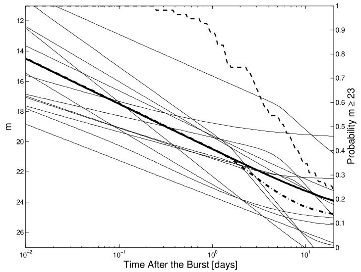
Figure 1: This figure shows 14 afterglow light-curves generated with parameters summarized in Zeh, Klose & Kann (zeh (2005)). The bold line and the bold dash-dotted line show the light curves of a typical afterglow ($\alpha_{1}=1,2\,$, $\alpha_{2}=2$, $t_{b}=1,5$ days, $m_{1}=20,5$, $m_{b}=21$, $m_{h}=25$) without and with a break respectively. The bold dashed line is the fraction of afterglows brighter than $23^{rd}$ magnitude at a given time (right hand scale). Nearly 90% of the afterglows are visible at magnitude $m\leqslant 23$, one day after the burst and 50%, 6 days after the burst.

Untriggered searches for GRB afterglows have already been attempted by a few teams, with really different observational parameters, but unsuccessfully. Rykoff et al. (rykoff05 (2005)) performed such a search with the ROTSE-III telescopes, covering a wide field at low sensitivity. On the contrary, Becker et al. (becker (2004)) have favoured a very deep survey, but with a very small field of view. They have found two interesting transient objects, which have recently been confirmed as flare stars (Kulkarni & Rau kulkarni06 (2006)). A similar attempt has also been performed by Rau et al. (rau (2006)), and once again an object behaving like a GRB afterglow has been detected, which was later identified as a flare star (Kulkarni & Rau kulkarni06 (2006)). Vanden Berk et al. (van (2002)) have searched GRB afterglows in the data of the SDSS survey. A very interesting transient was found, but it appeared to be an unusual AGN (Gal-Yam et al. galyam02 (2002)). So far no convincing optically selected GRB afterglow has been found. The failure of these searches is essentially the consequence of the scarcity of GRBs and of the faintness of their afterglows. The combination of these two factors implies that searches for orphan afterglows must be deep and cover several percent of the sky to have a reasonable chance of success. The search presented in this paper has a magnitude limit which is about the same as the search of Rau et al. (rau (2006)), but a sky coverage which is 50 times larger.

Our search for untriggered GRB afterglows uses images collected for the Very Wide Survey (one of the three components of the CFHT Legacy Survey, see http://www.cfht.hawaii.edu/Science/CFHTLS/) at the Canada-France-Hawaii Telescope. In the next section, we present the observational strategy used in this study. Section 3 introduces the Real Time Analysis System, with more details given in section 4 (catalog creation) and in section 5 (catalog comparison). In section 6 we analyze the performance of the RTAS during one full year of observation. Comparison with previous studies will be done in section 7. The last two sections encompass global considerations on afterglow search, the description of an ’optimal’ survey and our conclusions. All the web pages mentioned in this paper can be found at our web site: http://www.cfht.hawaii.edu/$\sim$grb/

2 The Canada-France-Hawaii Legacy Survey

The Canada-France-Hawaii Telescope (hereafter CFHT) is a 3.6 meter telescope located on the Mauna Kea in the Big Island of Hawaii. Built in the late 70’s, it has been equiped in 2003 with a high-performance instrument, MegaCAM. MegaCAM is a 36 CCD imager covering about 1 square degree field of view. Each CCD frame has $2\,048\times 4\,612$ pixels, for a total of $340\times 10^{6}$ pixels. It observes the sky through 5 filters (u* g’ r’ i’ z’), with a resolution of 0.185″per pixel. These characteristics, combined with the excellent climatic conditions at the site, provide very good quality images.

The CFHT Legacy Survey is the main observing program at the CFHT since june 2003. It is composed of 3 different surveys:

• The Wide Synoptic Survey, covering 170 deg² with all the 5 MegaCAM filters (u* g’ r’ i’ z’) down to approximatively i’=25.5. The main goal of this survey is to study large scale structure and matter distribution in the universe.

• The Deep Synoptic Survey which covers 4 deg² down to i’=28.4, and through the whole filter set. Aimed mainly at the detection of 2 000 type I supernovæ and the study of galaxy distribution, this survey will allow an accurate determination of cosmological parameters.

• The Very Wide Survey, covering 1 200 deg² down to i’=23.5, with only 3 filters (g’ r’ i’). As it has been initially conceived to discover and follow Kuiper Belt Objects, each field is observed several times, according to the strategy explained in Fig. 2.

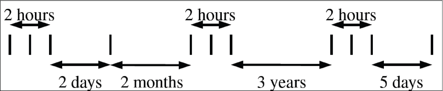
Figure 2: This diagram shows the observational strategy for one field of the Very Wide Survey. Each vertical line stands for one exposure, the exposure time depends on the filter, but is typically of the order of 100 seconds. 15 new fields or more are observed each month.

The images taken by the CFHT are pre-processed by a pipeline called Elixir (Magnier & Cuillandre magnier (2004)), which flattens and defringes each CCD frame and computes gross astrometry and photometry. About 20 minutes are needed to transfer the data from the telescope to Waimea and to process them with Elixir. Thanks to this pipeline, calibrated images are available in quasi-real time for the RTAS.

Although the Deep Synoptic Survey has a very interesting observational strategy, preliminary simulations have shown that the number of afterglow detections expected in near real time is very low compared to the Very Wide Survey. With relatively deep observations and very good quality images, the Very Wide Survey represents a credible opportunity to detect GRB afterglows independently of the prompt emission. Moreover, this is the only sub-survey with a well defined observational recurrence which can be used to compare images between them in order to detect variable, new, and/or vanishing objects, such as GRB afterglows. However, since we restrict the comparisons to objects detected in images taken during the same run, we are only able to detect objects with strong and fast variability.

3 The Real Time Analysis System

It is generally accepted that the most important quality in afterglow detection is speed. The Real Time Analysis System has been built to allow a quick follow-up of the afterglow candidates. Its goal is to analyze in quasi-real time ($<24$ hours) images of the Very Wide Survey to detect objects behaving like afterglows of GRBs. To permit quick automatic analysis, we have decided to work with catalogs of objects, and to compare between them catalogs of the same field of the sky taken at different times. Although the USNO-A2 catalog (Monet et al. monet98 (1998)) is used to astrometrically calibrate images, and the Digitized Sky Survey (DSS) to quickly characterize bright objects, we have no reference but ourself for objects fainter than $\sim 20$ magnitude, because of the depth and width of the Very Wide Survey.

Observations along the year at the CFHT are divided into runs, which are periods between two full moons lasting about 2 weeks. The optimization of the CFHT observational strategy during a run implies that we don’t know in advance when the images for the Very Wide Survey will be taken, because this depends on the weather, and on the pressure from other observational programs in queue observing mode. Two half-nights are generally dedicated to the Very Wide Survey, during which 15 fields at least are observed once to four times. This unpredictability is the reason why it is very important for the RTAS to be fully automatic. The main script is launched every fifteen minutes to check for new images to be processed, and the whole process is done without human intervention.

The RTAS has been installed on a dedicated computer at the CFHT headquarters. It is composed of many Perl scripts which prepare files and generate code for the other software used by the process. FITS to GIF conversion is done with IRAF, catalogs of objects with SExtractor, and the system core is coded for Matlab. Perl scripts also generate HTML and CSS outputs, which become accessible from the CFHT web page. CGI scripts used for catalog and comparison validation are also coded in Perl.

As shown in Fig. 3, the RTAS can be divided into two distinct parts, a night process for the catalog creation, and a day process for the catalog comparison. All results generated by the automatic pipeline are summarized on dynamic HTML web pages. Members of the collaboration are then able to check the process with a nice interface from any place which has internet connectivity.

Figure 3: This diagram shows the global mechanism of the RTAS pipeline and the interactions between the different components

4 Catalog Creation

The catalog creation process is composed of two main parts. The first part consists in the reduction of the useful information from about 700 MB, the size of an uncompressed MegaCAM image processed by Elixir, to a few tens of MB. The second part prepares the comparison between catalogs by astrometrically and photometrically calibrating objects, and sorting them according to their astrophysical properties.

Although images from the Very Wide Survey are processed one by one, the entire process works separately with each of the 36 CCD frames of an image, for two main reasons. First, the Elixir pipeline outputs one FITS file per CCD frame, so it is easier to use the same kind of data. Second, the astrometric calibration, which is the most time consuming operation in the catalog creation process, is made faster, but still accurate enough, since each CCD frame contains from 500 to a few thousand objects, depending on the filter used, the exposure time and the pointed sky region (see Fig. 8). Working with individual CCD frames has no major impact on the RTAS. The comparisons can be done within each CCD frame separately, since the pointing of the telescope is highly reproducible, and the CCD frames in images taken at different times overlap almost exactly.

In a first pass, the process detects the presence of new files in the directory where the Elixir pipeline pushes processed MegaCAM images, and waits for the image to be complete (with one file for each CCD frame). Images which are not part of the Very Wide Survey or which have already been processed are rejected; otherwise a backup of the files is done, allowing to reprocess them in case of an error in the treatment. In a second time, the FITS files of each CCD frame are converted into GIF images using IRAF, and then into JPEG images using the unix convert command. Then, the FITS header for each CCD frame is extracted and copied in an ASCII file. Some entries contained in this header are pushed as input parameters for SExtractor, used to create the catalogs.

In particular, an aproximative magnitude zero point (Mag0Point) is computed using header information. We have to mention here that the value of this self-computed Mag0Point does not take into account the climatic conditions of observations, especially seeing conditions and extinction due to clouds. It means that magnitudes of objects are relative, not absolute, although most of time the value is very close to the real one. Then, SExtractor is launched in order to create the catalog of objects, and the input parameters are added to the header as a reminder.

In parallel, an ASCII catalog of the same region of the sky is extracted from the USNO-A2.0 catalog, and used in an improved triangle matching method (Valdes et al. focas (1995)) in order to astrometrically calibrate our catalog. We achieve a precision of 0.6″or better for each CCD frame for the absolute positions of objects (see Table. 1). We have decided to not photometrically match objects with the USNO-A2.0 catalog, because the filters used do not correspond. At this step of the process, the catalogs contain one line per object, with the following parameters:

• A unique ID number

• The pixel coordinates, X and Y

• The J2000 coordinates, Right Ascension and DEClination

• The $\mu_{max}$ and the magnitude

• The FWHM (Full-Width at Half-Maximum)

• A flag computed by SExtractor: if its value doesn’t equal 0, the values of parameters are not reliable

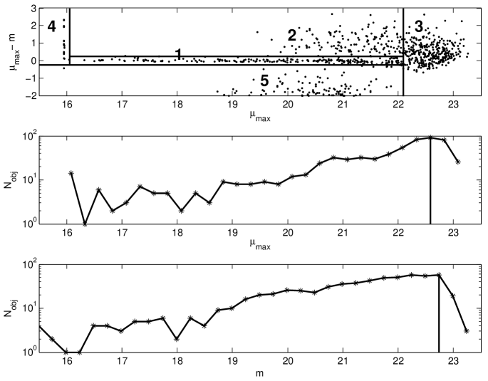
Figure 4: The upper figure shows our classification of objects in a plot $\mu_{max}-$magnitude versus $\mu_{max}$. We construct 4 classes of astrophysical objects: stars (1), galaxies (2), faint objects (3), saturated objects (4), and a class containing cosmic-rays (5). The lower two graphics represent the computation of the $\mu_{max}$ and magnitude completeness respectively.

In a next step, objects are sorted according to their astrophysical properties. By comparing $\mu_{max}$, the equivalent magnitude of the brightest pixel of the object, and the magnitude, we are able to find the ”line of stars”, and so to separate objects into 5 classes, of which 4 are astrophysical objects: stars, galaxies, faint objects, satured objects, and the last one contains cosmic-rays (see Fig. 4). Although this classification is quite arbitrary, especially for the faint objects boundary, it is very useful to compare objects between them and to reject non-astrophysical ones. Finally, $\mu_{max}$ and magnitude completeness will be used as cuts in the comparison process (see Fig. 4) while the ”line of stars” will be used to intercalibrate $\mu_{max}$ and magnitude between different images.

The processing of one image usually lasts between 5 and 15 minutes, mainly depending on the filter and of the observed region of the sky. The most time consuming steps are SExtractor and the astrometric matching. Most of the errors come from the USNO matching in CCD frames containing a very bright star or a large number of objects. These CCD frames are then flagged as unusable, and safe data are backed up on a special directory, allowing a quick re-processing of the image with the corrected code. Less than $0.35\%$ of the CCD frames produce an error (see table 1). Data of CCD frames correctly processed are saved in a database, which makes the post-process of the RTAS independent from the CFHT, and allows quick search of all kind of information in the whole set of data already processed.

Finally, all the results of the catalog creation process are summarized in real-time on an automatically generated HTML web page. In this page we summarize photometric, astrometric and classification values. Using an interactive script, collaboration members can check the results of the catalog creation process and decide to validate it. This validation allows starting the second part of the processing which involves the comparison of catalogs of the same field.

5 Catalog Comparisons

The goal of this process is to compare catalogs and extract from them a list of variable objects. The comparisons involve images of the same field, taken through the same filter. Exposure times have also to be of the same order. In a first step, catalogs are compared within a single night, by doublets (two images of the same field) or triplets (three images of the same field), depending on the Very Wide Survey observational strategy for this night. Differences between triple and double comparisons are discussed below. In a second step, the process selects for each field the best quality image of each night within the current run, and keeps it for an inter-night double comparison.

5.1 Triple Comparisons

Triple comparisons aim at extracting objects with strong magnitude variations, detecting asteroids and TNOs, and creating a reference catalog. Triple comparisons always involve images acquired during the same night.

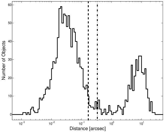
Figure 5: Histogram of the distance separating the nearest objects in two images. The largest peak is due to real astrophysical objects which are detected in the two images. The two vertical lines show the position tolerance and two times the position tolerance used for the matching of objects in the two images.

Before the beginning of the comparison, catalogs are ordered by ascending quality, defined by the mean number of astrophysical objects per CCD frame. The catalog with the highest quality (hereafter catalog 3) is taken as touchstone for the other two. All the calibrations are done with respect to this catalog. First, catalogs 1 and 2 are astrometrically matched to catalog 3 using the same method as for the USNO matching in the catalog creation. After this step we compute for each object the distance to its nearest neighbour in the other two catalogs. The nearest neighbour distance distribution is used to determine a position tolerance beyond which objects are considered to be distincts. This value is usually of the order of 1 pixel, or 0.2″(see Fig. 5). The objects are then classified into 3 categories depending on their distances with their nearest neighbours in the other two catalogs, wich are compared with the position tolerance derived above :

• If the smallest distance is lower than the position tolerance and the largest one is lower than twice the position tolerance, the object is classified as matched.

• If the smallest distance is lower than the position tolerance and the largest distance is higher than twice the position tolerance, the object is classified as suspect.

• Otherwise, the object is classified as single.

To summarize, matched objects are in all catalogs, suspect objects in two of them, and single objects are in only one catalog. A visual representation of this classification based on spatial proximity can be found in Fig. 6.

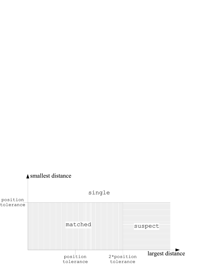
Figure 6: This diagram illustrates the spliting of astrophysical objects in matched, suspect and single objects in triple comparisons

Once all objects have been classified, matched stars are used to calibrate magnitudes, $\mu_{max}$ and FWHM to catalog 3. Matched objects which have been classified as stars, galaxies or faint objects in the catalog creation process are then searched for variability. The pipeline for the detection of variable objects works with 9 magnitude bins containing the same number of objects (except the last one). In each bin, an object is classified as photometrically variable if its magnitudes in the three catalogs verify the four following formulae at the same time:

$$\mid\leavevmode\nobreak\ m_{1}-m_{2}\mid+\mid\leavevmode\nobreak\ m_{1}-m_{3}\mid+\mid\leavevmode\nobreak\ m_{2}-m_{3}\mid\,\geqslant 3\times\Delta\leavevmode\nobreak\ m_{tot}$$ (1)

$$\mid\leavevmode\nobreak\ m_{1}-m_{2}\mid\,\geqslant\Delta\leavevmode\nobreak\ m_{1,2}$$ (2)

$$\mid\leavevmode\nobreak\ m_{1}-m_{3}\mid\,\geqslant\Delta\leavevmode\nobreak\ m_{1,3}$$ (3)

$$\mid\leavevmode\nobreak\ m_{2}-m_{2}\mid\,\geqslant\Delta\leavevmode\nobreak\ m_{2,3}$$ (4)

where $\Delta\leavevmode\nobreak\ m_{tot}$ is the median of the sum of the absolute value of the differences of magnitude for all matched objects in the bin, and $\Delta\leavevmode\nobreak\ m_{i,j}$ is the median of the absolute value of the difference of magnitude between matched objects of catalog i and j.

Equation (1) selects globally variable objects, and we ensure that objects are variable between each pair of catalogs with equations (2), (3) and (4). This choice is more sensitive to monotically variable objects.

Photometrically variable objects whose position is closer than 10 pixels to a CCD defect are removed from the list, as well at those above the $\mu_{max}$ completeness and flagged objects. Moving objects are detected among single objects using a simple pipeline which extracts single objects with a motion compatible between image 1 and 2, and image 2 and 3 in a chronological order. These objects are classified as asteroids.

Finally, a reference catalog containing the classification of all objects in the comparison is created. This reference catalog allows the detection of vanished or new objects in comparisons with images taken on other nights.

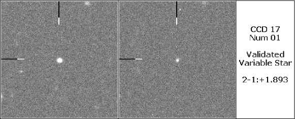
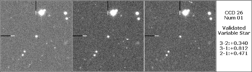
Figure 7: These two snapshots show two characterized variable stars in double (top) and triple (bottom) comparisons. For each images in which the object is detected, a thumbnail around its position is cut, and the difference of magnitude is computed. The coordinates of the first variable star are RA = 09:01:12.39, DEC = +17:29:09.22 and its magnitude in the first image is 20.21. The coordinates of the second variable star are RA = 04:50:40.66, DEC = +21:58:21.28 and its magnitude in the second image is 21.02.

5.2 Double Comparisons

Double comparisons are slightly different. One major difference is that the double comparisons do not allow fast and easy identification of the asteroids. As a consequence, these comparisons do not produce a list of astrometrically variable objects.

Like in triple comparisons, the first catalog is astrometrically matched to the second one, and a position tolerance is computed using pairs of nearest objects. Its value is similar to the one used in triple comparisons. Objects are classified as matched if their position difference is lower than the position tolerance, otherwise they are flagged as single objects. The magnitude, $\mu_{max}$ and FWHM of objects of the catalog 1 are calibrated to those in catalog 2, using matched stars. Photometrically variable objects are extracted with the same method as in triple comparisons, except that the value compared is the absolute value on the difference of magnitude, which must be greater than to 4 times the median value. Then, we apply a correction of the difference of magnitude to compensate for the difference of FWHM. This correction is essential because many objects classified as photometrically variable are in fact due to seeing difference between the 2 images, as the different background computed in SExtractor leads to variations of the magnitude. On all these objects we apply cuts on magnitude, $\mu_{max}$, CCD defects and flag.

When one of the two catalogs is also included in a triple comparison, a pipeline extracts objects that have been classified as matched in the triple comparison, and that are classified as single in the double one. This procedure allows to find objects which are classified as matched in the triple images but absent in the single image. The opposite cannot be done because the single image contains asteroids which appear as new objects and cannot be rejected.

5.3 Comparisons Output

The results of the classification of objects in comparisons are stored in a database and are easily available. This comparison database allows the detection of disappearing or appearing objects between nights and runs. To summarize a comparison, variable objects are gathered in two HTML web pages, for photometrically and astrometrically variable objects (see Fig. 7). These pages include a few graphics allowing an estimation of the quality of the comparison, a window of $250\times 250$ pixels centered on the objects showing them in each image, as well as an automatic cut-out of the field in the Digital Sky Survey, to confirm or not the presence of bright variable objects. An interactive script allows a member of the collaboration to characterize the nature of each variable object by choosing between one of these categories:

1. No comment (A)

2. Cosmic-ray (R)

3. CCD defect (R)

4. CCD edge (R)

5. Seeing (R)

6. Contaminated (R)

7. Faint (R)

8. Other (R/V)

9. Galaxy (V)

10. Variable star (V)

11. Trans-Neptunian Objects (TNO) (V)

12. Candidate (V)

Depending on this choice, the object will be classified as an asteroid (A), rejected (R) or validated (V), and displayed on the corresponding page. This procedure allows us to not only search GRB optical afterglows, but also to build catalogs of asteroids and photometrically variable sources. The results of this process, and the astrophysic characterization of the variable objects detected will be discussed in a forthcoming paper.

6 Statistics

This section presents detailed statistics for a sample of images taken during nearly one full year of observations. Statistics on catalogs represent the quality of our images, whereas statistics on comparisons show our efficiency to detect variable objects among astrophysical objects.

6.1 Catalogs

Table 1: Statistics of the catalog creation process. The 9 columns give respectively the code of the observing period or run (see footnote 6), the filter f, the galactic latitude b, the number of images $N_{obs}$, the number of square degrees observed $S_{obs}$, the median precision of the astrometric calibration $\delta_{pos}$, the limiting magnitude $M_{lim}$ (see text), and the number of astrophysical objects found par square degree $N_{obj}/deg^{2}$.

Run	f	b	$N_{obs}$	$S_{obs}$	$\delta_{pos}$	$M_{lim}$	$N_{obj}/deg^{2}$
		[deg]		[$deg^{2}$]	[”]		[$deg^{-2}$]
05AQ01	g’	+38	103	91.27	0.59	23.3	29 450
05AQ03	i’	+34	132	118.72	0.56	22.3	38 478
05AQ04	g’	+20	64	57.65	0.43	23.0	67 435
05AQ04	r’	+37	219	197.53	0.54	22.6	43 278
05AQ05	g’	+22	86	77.18	0.45	22.8	50 314
05AQ05	r’	-16	13	11.68	0.56	22.0	225 669
05AQ05	i’	-47	30	27.07	0.60	22.3	41 937
05BQ11	g’	-12	50	45.10	0.45	23.6	49 156
05BQ13	r’	+32	83	74.72	0.54	22.8	37 832
05BQ13	i’	-16	52	46.92	0.46	22.4	50 082
06AQ01	r’	+39	74	66.73	0.59	22.3	30 095
06AQ01	i’	-12	52	46.92	0.44	22.8	76 439
All	-	-	958	861.49	0.52	22.7	46 821

Table 1 presents some catalog statistics based on 958 observations. If we consider that the field of view of MegaCAM is $0.96\deg\times 0.94\deg$, the total sky coverage $S_{obs}$ is 864.5 deg². By properly processing 861.5 deg², the RTAS has an efficiency of 99.65% for the catalog creation process. We note that the USNO-A2.0 matching precision $\delta_{pos}$ is always better than 0.6″. The completness magnitude $M_{lim}$, which is strongly dependent on the filter used, is roughly distributed from $r^{\prime}=22$ to $g^{\prime}=23.6$, with a median value of 22.7. With the exception of the r’ filter images of 05AQ05 which were pointing near the galactic center, the total number of objects per square degree $N_{obj}/deg^{2}$ is about 50 000, depending on the filter, the seeing, and the observed region of the sky. Fig 8 summarizes the efficiency of the classification part of the catalog creation process (see Fig 4). It can be noticed that, while the number of astrophysical sources strongly varies, the number of cosmic-ray hits per CCD frame is nearly constant, except for 05BQ11, which has an exposure time twice than usual.

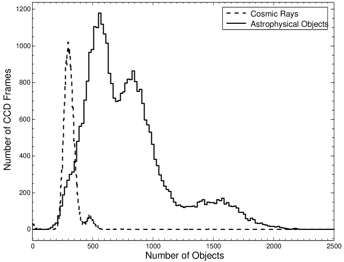
Figure 8: Histogram of the total number of astrophysical objects (solid line), and of the cosmic-ray hits (dashed line) in all the CCD frames studied. The nearly constant number of cosmic-ray hits, about 300 per CCD frame, is explained by the quasi constancy of the exposure time. The number of astrophysical objects, on the other hand appears much more variable as it depends strongly on the filter, and on the galactic latitude of the observations.

6.2 Triple Comparisons

As there is only a small chance of detecting GRB afterglows in triple comparisons (see Fig 9), they are mainly used to determine the true nature of objects, and to create the reference catalogs for the double comparisons. This is important because we expect a lot of asteroids and few variable objects, since the Very Wide Survey points to ecliptic plane and images are taken only 1 hour apart.

Table 2: Statistics for the triple comparisons process. The 8 columns give respectively the code of the observing period, the filter, the number of comparisons $N_{tri}$, the sky area involved in the comparisons $S_{tri}$, the limiting magnitude of the comparisons $M_{lim}$, the number of asteroids found in the comparisons $N_{ast}$, the number of variable sources found in the comparisons $N_{var}$, and the number of variable candidates per 10⁶ astrophysical objects found by the program $N_{6}$.

Run	Flt	$N_{tri}$	$S_{tri}$	$M_{lim}$	$N_{ast}$	$N_{var}$	$N_{6}$
			[$deg^{2}$]
05AQ01	g’	24	20.83	23.1	1 072	242	744
05AQ03	i’	31	27.55	22.0	912	362	585
05AQ04	g’	16	14.36	22.9	618	398	537
05AQ04	r’	50	44.94	22.5	2 543	842	657
05AQ05	g’	16	14.31	22.6	488	302	599
05AQ05	i’	10	9.02	22.0	288	88	387
05BQ11	g’	7	6.32	23.4	274	91	624
05BQ13	r’	20	17.95	22.6	1 129	270	746
05BQ13	i’	13	11.73	22.1	507	220	505
06AQ01	r’	18	16.19	22.1	749	152	638
06AQ01	i’	13	11.73	22.7	800	542	762
All	-	218	194.94	22.5	9 380	3 509	628

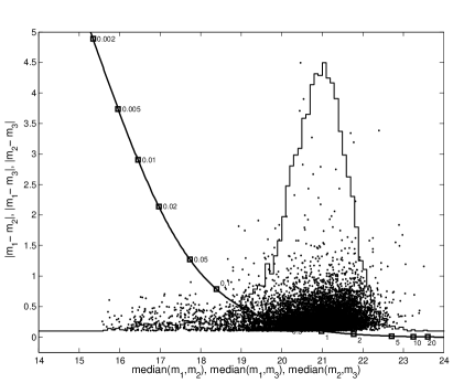
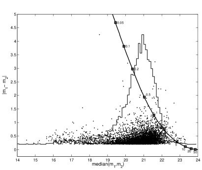
Figure 9: Objects detected variable by our automatic software, in triple (left) and double (right) comparisons. Each point represents one object in the comparison of a pair of images. The x-axis shows the median magnitude while the y-axis shows the magnitude difference between the two images. In the triple comparisons each object is represented by three points corresponding to the three possible pairs of images. The distribution of these variable objects is shown to illustrate the domain of sensitivity of our search (in magnitude and $\Delta mag$). For comparison we have also shown the track of a typical afterglow ($\alpha=1.2$, $M_{1}=21$ and $M_{host}=24$, see Sect.7), as a function of its age (in days) at the time of the first observation.

As shown in Table 2, 194.94 square degrees were compared in 218 triple comparisons. The magnitude completeness $M_{lim}$ is brighter than in the catalogs, because only matched objects were taken into account, so it represents in fact the completeness magnitude of the worst image of the triple comparison. 9 380 asteroids have been detected amongst 7 910 214 single objects. 3 509 matched objects were classified as variable amongst $5.10^{6}$ matched objects (only 1 per 1593 objects). In order to compare this value for all runs and filters independently from the number of objects, we used $N_{6}$, which is the number of variable objects per 1 000 000 matched objects. For the triple comparisons, $N_{6}$ is usually around 400 and 700. The difference of magnitude of variable objects as a function of their magnitude can be seen in Fig 9. 90% of variable objects are detected with a variation of less than 0.57 magnitude and 99% have a variation below 1.21. Objects with strong magnitude variation are usually variable stars or asteroids superimposed on a faint object.

6.3 Double Comparisons

Table 3: Statistics for the double comparisons process. The columns are identical to those of Table 2, except for $N_{sin}$ which is the number of new or vanished objects. This number is higher for the g’ filter images of 05AQ04 and 05AQ05 because halos of bright stars generate more fake objects in this filter.

Run	Flt	$N_{dou}$	$S_{dou}$	$M_{lim}$	$N_{sin}$	$N_{var}$	$N_{6}$
			[$deg^{2}$]
05AQ01	g’	28	24.84	22.6	10	317	1281
05AQ03	i’	24	21.66	22.3	2	463	790
05AQ04	g’	16	14.41	23.0	258	564	847
05AQ04	r’	62	55.87	22.5	132	1 231	796
05AQ05	g’	34	30.36	22.8	296	881	807
05AQ05	r’	3	2.66	21.5	0	80	132
05AQ05	i’	5	4.51	22.2	5	68	551
05BQ11	g’	7	6.32	23.6	15	94	522
05BQ13	r’	20	17.93	22.7	34	568	1387
05BQ13	i’	15	13.54	22.2	62	329	720
06AQ01	r’	20	17.95	22.5	64	449	1387
06AQ01	i’	13	11.68	22.4	97	656	980
All	-	247	221.71	22.5	975	5 700	825

247 double comparisons were performed for a total of 221.71 square degrees. The completeness magnitude $M_{lim}$ is a little better than the one in the triple comparisons statistics, because the best image of the triplet is selected. Except for comparisons of the g’ filter of 05AQ04 and 05AQ05, the number of objects detected as vanished or new, $N_{sin}$, is only a few per comparison, amongst a total of 7 638 326 single objects. $N_{6}$, the number of variable objects per $10^{6}$ matched objects, is higher than in triple comparisons, reaching a mean of 825. This is mainly due to two factors: first, inter-night comparisons detect objects which are variable on timescales of hours to days, including the objects detected in intra-night comparisons, and second, images taken 2 days apart are more sensitive to strong variations of the climatic conditions, resulting in more fake detections of variable objects due to seeing differences. Nevertheless, the number of detected variable objects stays low, with only 1 variable object for 1212 objects.

6.4 Characterization

Table 4: Characterization of variable objects of 05AQ01

	Triple comparisons		Double comparisons
	Number	%a	Number	%a
No comment	1	0.41	0	0
Cosmic-ray	10	4.13	31	9.48
CCD defect	42	17.36	100	30.58
CCD edge	2	0.83	9	2.75
Seeing	113	46.69	129	39.45
Contaminated	55	22.73	9	2.75
Faint	0	0	5	1.53
Other	0	0	0	0
Galaxy	2	0.83	5	1.53
Variable star	17	7.03	39	11.93
TNO	0	0	0	0
Candidate	0	0	0	0
Rejected	222	91.7	283	86.54
Validated	19	7.8	44	13.46

• percent of all variable objects

In Table 4 we provide an example of the characterization by a member of the collaboration of objects selected as variable by the automatic process for the run 05AQ01. About 90% of the variable objects are false detections. Most of them are due to seeing problems, CCD defects or contaminated objects. The validated objects are mostly variable stars. During this run we have not found any trans-neptunian object, and no object was interesting enough to be characterized as an afterglow candidate.

These statistics clearly show our conservative point of view about the selection of variable objects. The number of false detections like CCD defects or seeing problems could easily be reduced, at the expense of a lower sensitivity for afterglow detection. If there is little chance to detect a GRB afterglow within triple comparisons, their detection is fully possible in double comparisons. As shown in Fig 9, a typical afterglow would be detected as a variable object with $m\sim 21.5$, $\Delta\leavevmode\nobreak\ m\sim 1$ and $\Delta\leavevmode\nobreak\ t\sim 1$ day in the double comparison.

7 Estimations and Comparisons with other surveys

In this section, we compare the performance of our search for orphan afterglows using the Very Wide Survey with previous attempts. We do not discuss the estimation of the collimation factor, because all images taken have not been analyzed yet. This estimation will be the main purpose of a second paper.

We evaluate the performance of each survey along the following lines: we draw a sample of GRB afterglows and compute the number of them that will be detected by each survey taking into account its depth and strategy of observation.

We simulated afterglows with 5 random parameters: burst date, right ascension and declinaison, temporal decay slope $\alpha$ and magnitude at one day $M_{1}$. Light curves of simulated afterglows were chosen to be simple power law functions. The two intrinsic parameters $\alpha$ and $M_{1}$ were randomly drawn using probability laws fitted on 60 observed afterglows taken from various GCN notices (see Fig. 10). GRBs are produced at random times and isotropically on the sky.

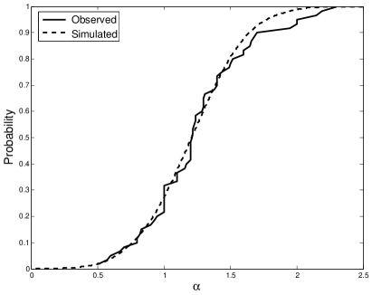
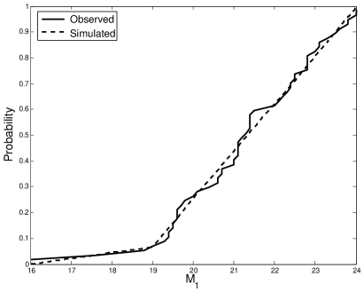
Figure 10: These two figures show the normalized distributions of $\alpha$ (left) and $M_{1}$ (right) for 60 observed afterglows and the distribution we choose to fit the data. Since there is no correlation between $\alpha$ and $M_{1}$, these values can be drawn independently

The number of afterglows generated depends on 2 parameters: $N_{\gamma}$ the number of bursts whose jet is directed towards the earth, which is independent of the observational strategy, and $\beta$ the collimation factor, which is simply the total number of bursts divided by $N_{\gamma}$. $\beta$ strongly depends on the limiting magnitude of the observations (Totani & Panaitescu totani02 (2002)). So, the number of afterglows generated for each survey is simply defined by $N_{\gamma}\times\beta$, where we choose $N_{\gamma}=800$, following Rau et al. (rau (2006)).

Each survey is described by the following parameters (see table 5):

• $S_{obs}$, the mean sky coverage in deg². In the computation of $S_{obs}$, we add up the areas of the images of the same field which are separated in time by more than the mean time of visibility of the afterglows.

• $\delta t$, the time between the two observations of each pair of images.

• $M_{lim}$, the mean completeness magnitude of observations

By using the completeness magnitude of each survey and the light-curves of simulated afterglows, we are able to derive their mean time of visibility $t_{vis}$, which is the time below which 50% of the afterglows remain visible in the images of the survey.

Table 5: Comparison of 4 programs dedicated to the search of GRB optical afterglows, $\beta$ have been chosen according to Totani & Panaitescu (totani02 (2002))

Survey	$\beta$	$S_{obs}$	$t_{vis}$a	$\delta t$	$M_{lim}$	$N_{exp}$b
		[deg2]	[days]
ROTSE-IIIc	2	65 550	0.07	0.02 days	18	0.6
Rau et al.d	15	55e	3.5	3 days	23	0.3
Very Wide	11	1 178	2.5	2 days	22.5	4.6
Optimal	21	250	7.5	7 days	24	5.6

• Mean time of visibilty of afterglows

• Number of afterglows expected

• Rykoff et al. (rykoff05 (2005))

• Rau et al. (rau (2006))

• $\sum_{i=1}^{7}\leavevmode\nobreak\ \big{[}(N_{sub,i}\times\frac{12}{\sum_{i}N_{sub,i}})\times(\frac{N_{night,i}}{3.5})\big{]}$, where $N_{sub,i}$ is the number of subfield and $N_{night,i}$ the number of nights of observation of each field

We choose to compare the observational strategy of the Very Wide Survey with 2 other surveys specially dedicated to GRB optical afterglow detection.

The survey used by Rykoff et al. (rykoff05 (2005)) has been performed with the ROTSE-III telescope. It has an extra wide sky coverage, but low sensitivity; that’s why the collimation factor is modest. Each field is observed twice within 30 minutes, and is considered as independent. This strategy is optimized for early afterglow detection. As shown in Table 5, half of the afterglows become undetectable about 2 hours after the burst. During this survey, 23000 sets were observed with a mean field size of 2.85 deg², so $S_{obs}=65500$. The distribution of magnitude along all sets in Rykoff et al. (rykoff05 (2005)) gives a completness magnitude $M_{lim}\sim 18$. According to Totani & Panaitescu (totani02 (2002)), $\beta$ is equal to 2 at this magnitude. By launching the simulation 50 times using this observing strategy, we can estimate the number of afterglows expected to be about 0.6. This is consistent with their analysis, since no GRB afterglow candidate has been discovered.

Another attempt has been performed by Rau et al. (rau (2006)) with the WFI Camera at the 2.2m MPI/ESO telescope in La Silla. The observational strategy was based on 7 fields, divided in sub-fields, and with multiple observations during a maximum of 25 nights in a row. Although 12 deg² were really observed, we upgrade the sky coverage to 55 independent square degrees observed twice within 3 days, using the mean time of visibility of afterglows, which is 3.5 days (see Table 5), and considering the difference of the observational strategy for each field (see Table 5^e). We choose to use the completeness magnitude given by Rau et al., which is $r=23$, although it seems to be in fact the limiting magnitude. This magnitude gives $\beta=15$ in Totani & Panaitescu (totani02 (2002)). The simulation was launched 50 times with these values. We estimate the number of afterglows expected in this survey to be 0.3 according to our simulation. This value is comparable with the results of their study: one object similar to an afterglow was found, although it has been later confirmed as a flare star (Kulkarni & Rau kulkarni06 (2006)).

Since the beginning of the Very Wide Survey, 4632 images were taken on 612 different fields of the sky. 1178 independent fields of $0.96\times 0.94\,deg^{2}$ have been observed at a mean magnitude of $r=22.5$, at which $\beta=15$ according to Totani & Panaitescu (totani02 (2002)). By using these values in 50 simulations, we estimate the number of afterglows in all of these images to be 4 to 5.

This simple simulation shows that the Very Wide Survey is to date the most adapted survey for the search of optical afterglows. Based on the predictions of Totani & Panaitescu (totani02 (2002)), we expect about 4 afterglows in the entire survey, ten times more than the survey of Rau et al..

8 Discussion of an optimal observational strategy

Although the observational strategy of the Very Wide Survey has not been built to search for GRB optical afterglows, our simulations show that the number of afterglows expected in this survey is ten times higher than in other dedicated programs. In this section, we will take advantage of the experience acquired from this work to further discuss the optimal observational strategy.

Given the rarity of optical GRB afterglows, the choice of an observational strategy is crucial to optimize their detection. Each strategy can be divided in two distincts part: the spatial part which defines the size and depth of the area observed, and the temporal part which defines the number of observations for each field and the time between observations. Since afterglows are very rare objects, and since their light-curves decrease like a power-law with time, a compromise has to be found between the depth and the width of the survey. A wide shallow survey favours the detection of ”early” and bright afterglows, but our simulation based on the ROTSE-III survey clearly shows that the chance of detecting such objects is very low because the beaming factor remains high during the early time of the burst. On the contrary, a deep survey favours late and faint detections. But, while the afterglows are much more numerous at faint magnitude, their detection is made more difficult by their slow decay and by the presence of the host galaxy. However, in our simulation, this kind of survey seems to be the most appropriate to search for optical afterglow.

Concretely, parameters that have to be defined to build an optimal survey are the sky coverage, the global observing strategy (number of observations and delay between them), and the depth of the observations. As we mentioned in the previous paragraph, when an afterglow reaches a certain magnitude, it starts to be hidden by its host galaxy, and its magnitude variation is not detectable anymore; therefore the mean magnitude of observed hosts of afterglows, $r=24$, seems to be a good value for the completeness magnitude. Due to the power-law decrease of its light curve, a typical afterglow doesn’t have strong magnitude variations at high magnitudes. So the observations have to be sufficiently spaced in time in order to have a difference of magnitude that allows the detection of the variability of the afterglow. At $r=24$, the mean time of visibility of afterglows is about 7.5 days (see Table 5). The maximum time between the two main observations can be chosen to be 7 days, but it can also be reduced to a few days in case of climatic or priority problems without any strong inconveniences.

Our experience clearly shows the necessity of a reference catalog in order to check the presence of variable objects and to detect new ones. When possible, the observed fields must be chosen to be part of an available survey at least as deep as the completeness magnitude, otherwise the fields have to be individually observed before the main observations within the survey, so these observations can be used to construct a reference catalog. Within the main observations, it is crucial to be capable to detect new or vanished objects, because a significant number of afterglows may appear or disappear between the two main observations. The search for such objects can only be processed by using the reference catalog, but, in order to be sure that the object is a non-moving stationary astrophysical source, there should be at least two observations for each main observation, taken during the same night. This will allow to fill the gaps between CCD frames and to construct an internal reference catalog, which will be very useful to characterize selected objects. Also a good idea is to refrain from pointing the ecliptic plane in order to avoid asteroids.

Since colors help neither for the detection nor for the characterization of the sources, all the observations can be done with the same filter. As this time of our investigation, we are not able to select a favourite filter, but since afterglows are at high redshift, a red filter would be a good choice. While such a survey is sufficient for the detection of the afterglows, a follow-up is still needed to confirm the nature of the detected objects. Since the confirmation of the variability of the object will most of the time take place during the second main observation, a fast identification is needed for confirmation with X-ray telescopes or big optical telescopes on the ground. A spectral analysis is also still conceivable, because the completeness magnitude $r=24$ corresponds to the limit magnitude below which a spectrum can be obtain with 8-10m class telescopes.

Given the above considerations, we can design an ”optimal” survey that will have $M_{lim}\sim 24$, $\delta t\lesssim 7$ days and $S_{obs}\sim 250$ deg². This survey would require about 7 full nights of observation with a CCD imager similar to MegaCAM at the CFHT, and 6 afterglows would be expected.

We conclude this section with an observation which has been a surprise for us: the very low background of astronomical sources which vary like GRB afterglows. It is interesting to note that a series of 3 to 5 exposures with a single filter was sufficient to eliminate nearly all the events which were strongly variable, like GRB afterglows. An essential ingredient in this task is the availability of at least one image taken months before, to check the existence in the past of the variable sources detected by the software.

9 Conclusion

In this paper, we have presented a new untrigerred search for optical GRB afterglows within the images of the Very Wide Survey at the Canada France Hawaii Telescope. In this survey, each field is observed three times during the same night and once 1 or 2 days later, allowing the detection of variable objects. Up to now, 1 178 independent fields of nearly 1 deg² have already been observed, down to $r^{\prime}=22.5$.

We have described in details the Real Time Analysis System ”Optically Selected GRB Afterglows”. This automatic pipeline, specially dedicated to an untriggered search of GRB afterglows, extracts variable, new and vanished objects, by comparing two or three catalogs of objects of images of the same field of the sky. Variable objects are displayed on a web page to be characterized by a human.

In order to quantify the efficiency of the process, statistics were computed on nearly one full year of observations. These statistics clearly show the quality of the images and of their processing, as well as our capability to detect variable objects within these images. Five to ten of 10 000 objects are classified as variable by the process, but only 10% of them are true astrophysical variable objects. In addition, we detect about 50 asteroids and a few new or vanished objects by comparison.

We finally performed a simulation of afterglow detection in order to compare our search with previous attempts, which have been unsuccessful. Our simulated afterglows are based on 60 real afterglows described in the GCNs. According to this simulation, the Very Wide Survey has an efficiency, which is ten times higher than previous searches.

We discussed an optimal survey for the search for GRB afterglows, based on the experience acquired from this work. Many considerations were taken into account, like the observational flexibility, the detection improvement and the follow-up opportunities for the confirmation of the object. This optimal survey, which can be completed with a few nights of observations with a telescope similar to the CFHT, will allow the detection of about 6 GRB afterglows according to the predictions of Totani & Panaitescu (totani02 (2002)). Our current experience demonstrates that the background of variable sources behaving like GRB afterglows is very low, allowing efficient searches based on the acquisition of few images of the same region of the sky taken hours to days apart with a single filter, with a reference taken 1 or 2 months before.

Since the RTAS is operational since November 2004, only one half of the fields observed within the Very Wide Survey have been searched for afterglows in real-time. Although a few objects that behaved like GRB afterglows have been found, none of them revealed to be a real afterglow. In the case that no afterglow is detected in the whole Very Wide Survey images, we will derive an upper limit of 6 orphan afterglows per 1 on-axis afterglow down to magnitude $r^{\prime}=22.5$. This value is consistent with the predictions of Totani & Panaitescu (totani02 (2002)) and Nakar et al. (nakar02 (2002)).

In a forthcoming paper, we will present the complete analysis of all variable objects found in the Very Wide Survey images. We will also discuss the estimation of the collimation factor of gamma-ray bursts.

- (1) Becker, A. C. et al. 2004, ApJ, 611, 418
- (2) Bloom, J. S., Frail, D. A., Kulkarni, S. R. 2003, ApJ, 594, 674
- (3) Dalal, N., Griest, K., & Pruet, J. 2002, ApJ, 564, 209
- (4) Frail, D. A. et al. 2001, ApJ, 562, L55
- (5) Gal-Yam, A., et al. 2002, PASP, 114, 587
- (6) Gal-Yam, A., et al. 2006, ApJ, 639, 331
- (7) Greiner, J., Voges, W., Boller, T., & Hartmann, D. 1999, A&AS, 138, 441
- (8) Groot, P. J., Vreeswijk, P. M., Huber, M. E. et al. 2003, MNRAS, 339, 427
- (9) Harrison, F. A., Bloom, J. S., Frail, D. A. et al. 1999, ApJ, 523, L121
- (10) Huang, Y. F., Dai, Z. G., & Lu, T. 2002, MNRAS, 332, 735
- (11) Kehoe, R., Akerlof, C., Balsano, R. et al. 2002, ApJ, 577, 845
- (12) Kulkarni, S. R., Djorgovski, S. G., Odewahn, S. C et al. 1999, Nature, 398, 389
- (13) Kulkarni, S. R., & Rau, A., 2006, ApJ Letter, 644, L63
- (14) Levinson, A., Ofek, E. O., Waxman, E., & Gal-Yam, A. 2002, ApJ, 576, 923
- (15) Magnier, E. A., Cuillandre, J-C., 2004, PASP, 116, 449
- (16) Mészáros, P., & Rees, M. J. 1997, ApJ, 476, 232
- (17) Moderski, R., Sikora, M., & Bulik, T. 2000, ApJ, 529, 151
- (18) Monet, D. B. A., Canzian, B., Dahn, C. et al. 1998, VizieR Online Data Catalog, 1252, 0
- (19) Nakar, A., Piran, T., & Granot, J. 2002, ApJ, 579, 699
- (20) Panaitescu, A., & Kumar, P. 2001, ApJ, 554, 667
- (21) Perna, R., & Loeb, A. 1998, ApJ, 509, L85
- (22) Piran, T., Kumar, P., Panaitescu, A., & Piro, L. 2001, ApJ, 560, L167
- (23) Rau et al., 2006, A&A, 449, 79
- (24) Rees, M. J., & Mészáros, P. 1992, MNRAS, 258, 41P
- (25) Rees, M. J., & Mészáros, P. 1994, ApJ, 430, L93
- (26) Rhoads, J. E. 1997, ApJ, 487, L1
- (27) Rhoads, J. E. 1999, ApJ, 525, 737
- (28) Rykoff, E. S., Aharonian, F., Akerlof, C. W. et al. 2005, ApJ, 631, 1032
- (29) Sari, R., Piran, T., & Narayan, R. 1998, ApJ, 497, L17
- (30) Sari, R., Piran, T., & Halpern, J. P. 1999, ApJ, 519, L17
- (31) Totani, T., & Panaitescu, A. 2002, ApJ, 576, 120
- (32) Valdes, F. G. et al. 1995, PASP, 107, 1119
- (33) Vanden Berk, D. E. et al, 2002, ApJ, 576, 673
- (34) Wei, D. M., & Lu, T. 2000, ApJ, 541, 203
- (35) Wijers, R. A. M. J., Rees, M. J., & Mészáros, P. 1997, MNRAS, 288, L51
- (36) Zeh, A., Klose, S. & Kann, D. A. 2005, ApJ, 637, 889
- (37) Zhang, B., & Mészáros, P. 2002, ApJ, 571, 876