Dark energy constraints from lensing-detected galaxy clusters

Abstract

We study the ability of weak lensing surveys to detect galaxy clusters and constrain cosmological parameters, in particular the equation of state of dark energy. There are two major sources of noise for weak lensing cluster measurements: the “shape noise” from the intrinsic ellipticities of galaxies; and the large scale projection noise. We produce a filter for the shear field which optimizes the signal-to-noise of shape-noise-dominated shear measurements. Our Fisher-matrix analysis of this projected-mass observable makes use of the shape of this mass-function, and takes into account the Poisson variance, sample variance, shape noise, and projected-mass noise, and also the fact that the conversion of the shear signal into mass is cosmology-dependent. The Fisher analysis is applied to both a nominal 15,000 deg² ground-based survey and a 1000 deg² space-based survey. Assuming a detection threshold of $S/N=5$, we find both experiments detect $\approx 20,000$ clusters, and yield 1-$\sigma$ constraints of $\Delta w_{0}\approx 0.07$, $\Delta w_{a}\approx 0.20$ when combined with CMB data (for flat universe). The projection noise exceeds the shape noise only for clusters at $z\lesssim 0.1$ and has little effect on the derived dark-energy constraints. Sample variance does not significantly affect either survey. Finally, we note that all these results are extremely sensitive to the noise levels and detection thresholds that we impose. They can be significantly improved if we combine ground and space surveys as independent experiments and add their corresponding Fisher matrices.

I Introduction

Constraining the dark energy equation of state and density parameters is the objective of many cosmologists; not few of them have considered using present or future cluster data to attain this goal. Cluster methods rely mostly on detection and counting of objects using some mass-indicating observable; for constraining cosmology there are 4 ways of finding clusters: optical emission by galaxies, the X-ray emission by the hot intracluster medium, the Sunyaev-Zeldovich effect on CMB, and gravitational lensing.

X-ray clusters received a lot of attention from cosmologists Henry & Arnaud (1991); Henry (1997); Wang & Steinhardt (1998); Kitayama & Suto (1997); Bahcall & Fan (1998); Levine,Schulz & White (2002), then SZ clusters Eke,Cole & Frenk (1996); Holder,Haiman & Mohr (2001); Weller,Battye & Kneissl (2002); Battye & Weller (2003). See Haiman,Mohr & Holder (2001); Majumdar & Mohr (2003, 2004) for thorough comparisons between the efficiency of extracting cosmological information from X-ray and SZ clusters and also for using complementary studies of the CMB and supernovae distance measurements to improve constraints. For optically-detected cluster surveys and their results see the work of Bahcall et al (2003a, b, c); Gladders (2000); Gladders & Yee (2005).

The main issue with the X-ray, optical, and SZ clusters is the so-called mass-observable relation: cluster masses are not measured directly, but they are estimated from the real observables, such as the X-ray temperature or flux or the SZ integrated flux. But, as pointed out in (Majumdar & Mohr, 2003), the mass-observable relation can have non-standard redshift evolution and, if not carefully calibrated, the constraints on dark energy parameters are compromised. Cross-calibration of the mass-observable relations between different types of surveys could, though perhaps not very efficiently, ameliorate the situation; more recently, self-calibration using the sample variance of the counts due to clustering of clusters has been proposed as a non-costly alternative to cross-calibration, eg see Lima & Hu (2004); Hu & Kravtsov (2003).

Weak gravitational lensing detects clusters via the slight distortions imparted on the images of background galaxies. The lensing information is obtained from shear maps: clusters are detected using some filtering technique that finds the points where the signal-to-noise ($S/N$) is high enough for us to conclude that there is an overdensity. The filtered shear is the mass observable. The relation of this observable to the projected mass is very simple and unambiguous. The strength of the lensing method is this lack of ambiguity in the mass-observable relation.

A difficulty arises because such a point with high $S/N$ does not necessarily correspond to a virialized cluster: it could also be the result of unvirialized large scale structure projected along the line of sight, or the superposition of multiple unrelated lower-mass objects Hennawi & Spergel (2004); Hamana,Takada & Yoshida (2004). Even for virialized clusters, there will be substantial scatter between the projected-mass observable and the traditionally defined virial mass Croft & Metzler (2000). But there is in fact no underlying need for lensing observables to correspond to other cluster observables, nor even to a dynamical definition of mass. We will argue that counts of projected-mass overdensities are just as useful for cosmology as counts of virialized halos.

In this paper we study how well a $4-$dimensional parameter space can be constrained using weak-lensing-detected clusters. The parameters in question are $\Omega_{m}$ (the matter density parameter), $w_{0},w_{a}$and $\sigma_{8}$ (the amplitude of the matter power spectrum). $w_{0}$ and $w_{a}$ define the time-varying equation of state of dark energy: $w(a)=w_{0}+(1-a)w_{a}$. We use as examples two proposed future surveys, a ground-based Large Survey Telescope (LST) lst and the space-based Supernova Acceleration Probe (SNAP) snap . We first review the role of cluster-mass observables in constraining cosmology. In §III we describe a filter based on $S/N$ maximization of shear measurements that determines the minimum detectable mass of an object placed at a certain redshift. In §IV we calculate the cosmological constraints obtained when assuming that the intrinsic ellipticities of background galaxies are the only source of noise. In §V we treat the large scale structure projection errors and in §VI we draw some conclusions.

The fiducial $\Lambda$CDM cosmological model for this whole paper is: flat universe, $\Omega_{m}=0.27$, $\sigma_{8}=0.9$, $w_{0}=-1$, $w_{a}=0$, $h=0.72$, $\Omega_{b}\,h^{2}=0.024$, consistent with the first-year WMAP results Spergel et al. (2003).

II Mass Observables and Cosmology

Any observable statistic can be used as a cosmological test, as long as (1) it can be measured on the real Universe, and (2) its value can be predicted as a function of the cosmological parameters of interest. The utility of the statistic depends upon: the accuracy with which the measurement can be made; the accuracy with which the predictions can be made; and the sensitivity of the statistic to the parameters. To forecast the parameter accuracies, as we aim to do here, we need only estimate these three characteristics of the statistic.

Overdensity-counting methods have as their statistic the distribution $dN/d\Omega\,dz\,d\mbox{$\tilde{M}$}$ of “clusters” in a solid angle $\Omega$ vs redshift as a function of some observable quantity $\tilde{M}$ [the clustering of these overdensities may be an additional statistic]. In an ideal world, the observable would be the virial mass $M$, because there exist analytic frameworks Press & Schechter (1974); Sheth & Tormen (1999) for predicting their distribution, a.k.a. the mass function. To constrain dark energy at interesting levels, the mass function must be predicted to an accuracy that will undoubtedly require $N$-body simulations, not just the analytic frameworks. For more recent work on mass functions and their accuracy see for instance Jenkins et al (2001); Warren et al (2005). This is also of course true for the real-life substitutes for virial mass: the x-ray flux/temperature, the SZ decrement, galaxy counts, and the lensing shear. There is no long-term advantage to an observable that is closely correlated to the virial mass. The ultimate utility of these methods will depend upon the fidelity of the numerical predictions, and here the lensing method is clearly superior. The shear prediction needs only the mass distribution, and 83% of the mass is easily-modelled collisionless dark matter. X-rays and SZ decrements depend fully upon the more complex baryon distribution, and the electron temperature as well. Cooling and density fluctuations particularly affect the x-ray predictions. Galaxy counts are even more difficult to predict. It would be bold to assert that modelling will ever predict any of these observables other than the shear to the percent-level accuracies we will someday desire.

Are analytic mass functions adequate for forecasting parameter accuracies? To be so, they must roughly—but not exactly—predict the number of peaks in $\tilde{M}$, so that our Poisson errors are properly estimated. When $\tilde{M}$ is a projected mass measurement, several numerical studies Hennawi & Spergel (2004); Hamana,Takada & Yoshida (2004) show that up to tens of percent of detections can be “false positives” in the sense of having no corresponding virialized cluster, and some virialized clusters are missed. The Poisson statistics are grossly perturbed only when the $S/N$ threshold is low enough that measurement-noise peaks overwhelm the mass signals.

The analytic model must also properly capture the dependence upon cosmological parameters. The “false positives” when $\tilde{M}$ is the projected mass are not virialized, but they are real structures whose abundance will scale with $\sigma_{8}$ and the linear growth rate in a manner not grossly different from the virialized structures Weinberg & Kamionkowski (2003).

The projections which distinguish lensing-derived projected masses from dynamical masses can be divided into two classes: first, there are projections between mass structures that are widely separated along the line of sight, in which case there is no angular correlation between the projected halos. In §V we treat such projections as a source of random noise on the mass determinations of detected clusters induced by projection of below-threshold halos.

The second difference between lensing mass and virial mass is that the former includes all the structure along the line of sight that is correlated with the mass peak, not just the virialized (or unvirialized) core. The lensing “mass function” is therefore distinct from the mass function of virialized halos, but it is just as well defined. We will simply assume for this paper that the projected-mass function is equal to the virial-mass function produced by the Press-Schechter formalism and related techniques, in the absence of numerical or analytic evidence that the two differ dramatically.

We conclude that the distinction between the weak-lensing projected-mass observable $\tilde{M}$ and the virial mass $M$ will not be a barrier to its use as a precision cosmological constraint, and that we can use the virial mass functions for approximate forecasts of these constraints. Naturally, for accurate constraints on dark energy, one will have to use a lensing mass function derived from numerical simulations.

III The minimum detectable mass

Given a cluster at some redshift, we would like to determine the smallest value of its mass such that it could be detected through weak lensing (WL) effects. In this section we assume that the intrinsic ellipticities of the galaxies represent the dominant source of noise for the projected mass measurement. We shall test this assumption in §V, where we consider the large scale projection effects.

III.1 S/N maximization

As mentioned in the introduction, for WL measurements the observable is the shear, which encodes information about the direction and magnitude of the distortion of background galaxies images. The components of the shear contain derivatives of the deflection angle with respect to the apparent position of the source galaxy. In the case of WL, distortions and magnifications are so small that we can very well approximate the relation between the components of the induced shear $(\gamma_{1},\gamma_{2})$ and those of the measured image ellipticity $(e_{1},e_{2})$ in the following way (see Dodelson (2003) for example):

$$e_{i}\approx 2\gamma_{i}+\tilde{e}_{i}\,,\qquad i\in\{1,2\}\;.$$ (1)

$(\tilde{e}_{1},\tilde{e}_{2})$ represents the intrinsic ellipticity of the galaxy. From measurements of $N$ galaxies, the shear can be estimated with the accuracy:

$${\rm Var}(\gamma_{1})=\frac{\sigma_{\gamma}^{2}}{N}\,,$$ (2)

where $\sigma_{\gamma}$ is the uncertainty in the measurement of one galaxy. For a detailed investigation of the shape noise, we refer the reader to Bernstein & Jarvis (2002). An approximate expression is Bernstein (2006):

$$\sigma_{\gamma}\approx\frac{\langle e_{1}^{2}\rangle^{1/2}}{2}\,.$$ (3)

A filtered shear map is used to detect clusters by selecting the points where the $S/N$ peaks above some threshold, $(S/N)_{\rm{min}}$. But the filtered shear values are also used in the interpretation of the detected clusters. We are at liberty to choose any filtering method we wish, provided we can tie its results to a physical quantity for which there exists a theory. We choose to normalize our filter to reproduce the virial mass when applied to canonical clusters, namely spherically symmetric objects, with NFW density profiles in the context of a $\Lambda$CDM cosmology—i.e. what we expect the average (if not typical) cluster profiles to be. This close scaling will allow us to use the well-studied and tested mass function theory to predict the number of detectable clusters. Therefore, the two requirements for our filter are first that it yield a value closely related to the virial mass for canonical clusters; and second, that the virial mass estimator produce a maximum $S/N$ from the shear map.

For a circularly symmetric lens, the shear has only one component, tangent to the annulus about the cluster center. We define our mass estimator as a weighted sum of the shears in such annuli:

$$\mbox{$\tilde{M}$}=\sum_{k,i}w(\theta_{k},z_{i})\gamma_{T}(\theta_{k},z_{i})\,,$$ (4)

where $k$ designates the annulus with angular radius $\theta_{k}$, $\gamma_{T}(\theta_{k},z_{i})$ is the measured shear of annulus $k$ on sources in redshift bin $i$, and $w(\theta_{k},z_{i})$ is the weight on this shear. The variance of this estimator is:

$${\rm Var}(\mbox{$\tilde{M}$})\!=\!\!\!\sum_{k,k^{\prime},i,j}\!\!w(\theta_{k},z_{i})w(\theta_{k^{\prime}},z_{j}){\rm Cov}\left[\gamma_{T}(\theta_{k},z_{i})\gamma_{T}(\theta_{k^{\prime}},z_{j})\right].$$ (5)

When the noise of the intrinsic ellipticities of galaxies is dominant, the contributions of different redshift bins to the estimator variance are uncorrelated and the above expression reduces to:

$${\rm Var}(\mbox{$\tilde{M}$})=\sum_{k,i}w(\theta_{k},z_{i})^{2}\ \,{\rm Var}(\gamma_{T}(\theta_{k},z_{i}))\,.$$ (6)

The desired maximization of $S/N$ is obtained for the following set of $w$’s:

$$w(\theta_{k},z_{i})\propto\frac{\gamma_{T}(\theta_{k},z_{i})}{{\rm Var}(\gamma_{T}(\theta_{k},z_{i}))},\;\forall\,k,i\,.$$ (7)

The normalization constant in equation (7) is set by the first property of our filter: if the real clusters have NFW profiles and the real cosmology is $\Lambda$CDM, then the estimator must return the virial mass of the clusters. Thus, the constant is:

$$\mathcal{C}=\frac{M_{\rm{vir}}}{\sum_{k,i}(\gamma_{T}^{\Lambda CDM}(\theta_{k},z_{i}))^{2}/\rm{Var}(\gamma_{T}(\theta_{k},z_{i}))}\,.$$ (8)

The shear and the optimal weight separate into a part depending only on the lens properties, and a part depending only on the lens and source redshifts. For redshift bin $i$ we write:

$$\gamma_{T}(z_{i},z_{d})=\frac{\int_{z_{i}}^{z_{i+1}}dz_{s}\,\mathcal{P}(z_{s})Z(z_{s},z_{d})\,\gamma_{\infty}(z_{d})}{\int_{z_{i}}^{z_{i+1}}dz_{s}\,\mathcal{P}(z_{s})}\,.$$ (9)

In the above equation, $\gamma_{\infty}(z_{d})$ is the shear of a hypothetical source at infinity, $\mathcal{P}(z_{s})$ is the redshift distribution of source galaxies (see §III.2) and $Z$ is given by:

$$Z(z_{s},z_{d})=\left\{\begin{array}[]{ll}\frac{D_{ds}}{D_{s}}&\mbox{if $z_{s}>z_{d}$}\\ 0&\mbox{otherwise}\end{array}\right.\,,$$ (10)

where $D_{ds}$ is the angular-diameter distance between the lens and the source and $D_{s}$ is the angular-diameter distance between theobserver and the source. Throughout this paper we consider only the case of a flat universe. In the limit of an infinite number of redshift bins and if we introduce the shear per unit mass for the canonical cluster, $\tilde{\gamma}_{\infty}$, equation (9) becomes:

$$\gamma_{T}(z_{i},z_{d},\theta)=\mbox{$\tilde{M}$}Z(z_{i},z_{d})\,\tilde{\gamma}_{\infty}(z_{d},\theta)\,.$$ (11)

To make the notation easier, we shall ignore the dependence on $z_{d}$ of $\gamma_{T}$ and $\tilde{\gamma}_{\infty}$. Using the normalization constant defined by equation (8), we obtain for the noise of the measurement:

$${\rm Var}(\mbox{$\tilde{M}$})=\left(\sum_{k,i}\frac{\tilde{\gamma}_{\infty}(\theta_{k})^{2}Z(z_{i},z_{d})^{2}}{{\rm Var}(\gamma_{T}(\theta_{k},z_{i}))}\right)^{-1}\,,$$ (12)

with $\tilde{\gamma}_{\infty}$ and $Z$ evaluated for the NFW profile and a $\Lambda$CDM cosmology. ${\rm Var}(\gamma_{T}(\theta_{k},z_{i}))$ is given by equation (2):

$${\rm Var}(\gamma_{T}(\theta_{k},z_{i}))=\frac{\sigma_{\gamma}^{2}}{N(\theta_{k},z_{i})}\,,$$

where $N(\theta_{k},z_{i})$ is the number of galaxies in redshift bin $i$ sheared in annulus $k$ and

$$N(\theta_{k},z_{i})=\int_{z_{i}}^{z_{i+1}}\int_{0}^{2\pi}\int_{\theta_{k}}^{\theta_{k+1}}dz_{s}d\varphi\,d^{2}\theta\mathcal{P}(z_{s})n(\theta,\varphi)\,.$$

If the annuli are dense enough and using the above relations, as well as equations (7) and (8), we can rewrite the mass estimator of an NFW cluster as:

$$\mbox{$\tilde{M}$}=M_{\rm{vir}}\,g({p_{\alpha}})\,,$$ (13)

where the $p_{\alpha}$’s generically denote cosmological parameters. $g({p_{\alpha}})$ is the change of the estimated mass from the true virial mass if the cosmology is different from $\Lambda$CDM:

$$g(p_{\alpha})=\frac{\int_{0}^{\infty}dz_{s}\mathcal{P}(z_{s})\int_{0}^{\theta_{lim}}d\theta\,\theta\tilde{\gamma}_{T}(\theta,z_{s},z_{d})\tilde{\gamma}_{T}^{m}(\theta,z_{s},z_{d})}{\int_{0}^{\infty}dz_{s}\mathcal{P}(z_{s})\int_{0}^{\theta_{lim}}d\theta\,\theta\tilde{\gamma}_{T}^{2}(\theta,z_{s},z_{d})}.$$ (14)

$\tilde{\gamma}_{T}(\theta,z_{s},z_{d})$ is the tangential shear per unit mass for a $\Lambda$CDM cosmology. $\tilde{\gamma}_{T}^{m}$ is the shear one will measure in the real cosmology, possibly other than $\Lambda$CDM.

Note that if $\gamma_{\infty}(\theta)$ is independent of cosmology, then $g(p_{\alpha})$ is simply a ratio of angular-diameter distances. More generally, the parameters of the NFW profile of a cluster of given $M_{\rm vir}$ will depend upon cosmology.

The variance of the mass estimator, written also in the case of continuous annuli is:

$${\rm Var}(\mbox{$\tilde{M}$},z_{d})=\frac{\sigma_{\gamma}^{2}}{2\pi n}$$ (15)

$$\times\left(\int_{0}^{\infty}dz_{s}\mathcal{P}(z_{s})Z^{2}(z_{s},z_{d})\int_{0}^{\theta_{lim}}d\theta\,\theta\,\tilde{\gamma}_{\infty}^{2}(\theta,z_{d})\right)^{-1}.$$

Here we have considered a constant angular concentration of galaxies. For the upper bound of the second integral in the above equation we take $\theta_{lim}=\frac{2\,R_{vir}}{D_{d}}$, with $R_{vir}$ the virial radius of the measured cluster. This choice of $\theta_{lim}$ seems a reasonable trade-off for looking widely enough to get a significant signal without too much contamination by other lensing structures.

A cluster is detectable if its mass estimator has a minimum value of

$$\tilde{M}_{\rm min}(z_{d})=(S/N)_{\rm min}\>\sqrt{{\rm Var}(\mbox{$\tilde{M}$},z_{d})}\,,$$ (16)

where ${(S/N)_{\rm min}}$ is the detection threshold that we choose for our measurement and ${\rm Var}(\mbox{$\tilde{M}$},z_{d})$ is given by equation (15).

Let us emphasize again that only in the case of a canonical cluster (NFW profile in a $\Lambda$CDM cosmology) does our estimator translate the shear signal into the cluster’s virial mass. If the cosmology is changed from $\Lambda$CDM, the same shear signal results from a different virial mass, as one can see from equation (13). But even so we are still able to find and count objects. Since $N$-body simulations will yield the functional dependence on cosmology of the difference between the estimated and the virial mass, we can still understand our counts and know how to extract cosmological constraints from them. The measurement is well-defined for clusters that do not have the canonical NFW profile, but in this paper we do not attempt numerical simulations to derive the effect of this difference on WL cluster counts.

III.2 Distribution of sources and the NFW shear

We now present a few steps that we take in order to compute the variance given by equation (15).

We assume the source galaxies to have the redshift distribution introduced by Smail et al. (1995) and used in many other works, e.g. see Bartelmann & Schneider (1999); Weinberg & Kamionkowski (2003); Hennawi & Spergel (2004):

$$\mathcal{P}(z)=\frac{1}{2\,z_{0}^{3}}\,z^{2}\,\exp{(-z/z_{0})}\,.$$ (17)

The mean of this distribution is $\langle z\rangle=3z_{0}$ ; the characteristics of the fiducial survey will set the value of $z_{0}$.

As already specified, we optimize our filter for spherically symmetric clusters with NFW profiles and in a $\Lambda$CDM cosmology.

A thorough treatment of NFW lenses is given by Bartelmann (1996), as well as by Wright & Brainerd (2000). The shear due to NFW mass distributions is:

$$\gamma_{\rm NFW}(x)=\left\{\begin{array}[]{lcl}\frac{r_{s}\,\delta_{c}\,\rho_{c}}{\Sigma_{crit}}\,g_{<}(x)&\mbox{$,\;$ $x<1$ }\\ \frac{r_{s}\,\delta_{c}\,\rho_{c}}{\Sigma_{crit}}\,\left[10/3+4\ln(1/2)\right]&\mbox{$,\;$ $x=1$ }\\ \frac{r_{s}\,\delta_{c}\,\rho_{c}}{\Sigma_{crit}}\,g_{>}(x)&\mbox{$,\;$ $x>1$}\,,\end{array}\right.$$ (18)

where $x=\frac{\theta D_{d}}{r_{s}}$ and $r_{s}$ is the scale radius of the halo. $\delta_{c}$ is the characteristic overdensity and $\rho_{c}(z)=\frac{3\,H^{2}(z)}{8\pi G}$ is the critical density of the universe. The characteristic overdensity is related to the concentration parameter of halos by the condition that the mean density within the virial radius $R_{vir}$ should be $\Delta_{vir}\rho_{c}$, where $\Delta_{vir}=200$ for NFW: $\,\delta_{c}=\frac{\Delta_{vir}}{3}\,\frac{c^{3}}{\ln(1+c)-\frac{c}{1+c}}$ (see Navarro,Frenk & White (1996) for more details). The functions $g_{<}$ and $g_{>}$ are independent of cosmology and of cluster parameters and are given by:

$$\begin{array}[]{lc}g_{<}(x)=\frac{8\tanh^{-1}\sqrt{\frac{1-x}{1+x}}}{x^{2}\sqrt{1-x^{2}}}+\frac{4}{x^{2}}\ln\left(\frac{x}{2}\right)-\frac{2}{x^{2}-1}\\ \mbox{$\;\;\;\;$}\mbox{$\;\;\;\;$}\mbox{$\;\;\;\;\;$}+\frac{4\tanh^{-1}\sqrt{\frac{1-x}{1+x}}}{(x^{2}-1)\sqrt{1-x^{2}}}\,;\par\end{array}$$

$$\begin{array}[]{lc}g_{>}(x)=\frac{8\tan^{-1}\sqrt{\frac{x-1}{x+1}}}{x^{2}\sqrt{x^{2}-1}}+\frac{4}{x^{2}}\ln\left(\frac{x}{2}\right)-\frac{2}{x^{2}-1}\\ \mbox{$\;\;\;\;$}\mbox{$\;\;\;\;$}\mbox{$\;\;\;\;\;$}+\frac{4\tan^{-1}\sqrt{\frac{x-1}{x+1}}}{(x^{2}-1)^{3/2}}\,.\par\end{array}$$

Given a cosmology and a halo of some mass and at some redshift, we need the concentration parameter $c$ in order to compute the characteristic overdensity and the scale radius. We assume a relation between $c$ and $M$ as given by Navarro,Frenk & White (1996).

III.3 Mass thresholds for nominal surveys

In order to see the redshift dependence of the WL mass thresholds provided by equations (15) and (16), we consider the examples of possible two future surveys: a Large Survey Telescope (LST) from the ground, and the space-based Supernova Acceleration Probe (SNAP). We assume for both surveys $\sigma_{\gamma}=0.3$. For LST we use a distribution of galaxies with a mean redshift of 1, i.e. $z_{0}=0.33$. The angular concentration of sources is $n=30$ galaxies/arcmin² and the survey area is $\mathcal{A}=15000$deg². In the case of SNAP, we take $z_{0}=0.5$, $n=100$ galaxies/arcmin² and $\mathcal{A}=1000$deg². For a fixed $z_{d}$ we compute ${\rm Var}(\mbox{$\tilde{M}$},z_{d})$ as given by equation (15) and then we find the smallest value of $\tilde{M}$ verifying  (16). This value gives $\mbox{$\tilde{M}$}_{\rm min}(z_{d})$. The solid lines in figure 1 show the detection thresholds for both instruments using the NFW definition of the virial mass. To compute the cluster abundance, we shall convert to the Sheth-Tormen definition of virial mass and $\mbox{$\tilde{M}$}_{\rm min}$ will rise by approximately 30% for $z_{d}<0.4$.

Not surprisingly, the detection threshold for the space telescope is much lower than that of the ground telescope (3 or 4 times for small redshifts and almost an order of magnitude for redshifts higher than 1). In compensation, LST covers a substantially larger area of the sky, so in the end both telescopes can detect similar abundances of clusters.

Using equation (19), we obtain $\approx 21500$ detectable clusters for LST and $\approx 17500$ for SNAP if $(S/N)_{\rm{min}}=5$. If $(S/N)_{\rm{min}}=10$, the numbers are 1600 and 2200 respectively. As the cluster mass function is very steep, the derived cluster counts and resultant cosmological constraints are quite sensitive to assumptions about input noise levels ($\sigma_{\gamma}$, $n$, and $z_{d}$) and $(S/N)_{\rm min}$.

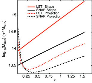
Figure 1: Minimum detectable mass for LST and SNAP when $\rm{(S/N)_{min}}=5$. The solid lines represent $M_{\rm{min}}$ when the intrinsic ellipticity noise dominates the measurement. The dotted lines represent $M_{\rm{min}}$ when the projection noise is dominant.

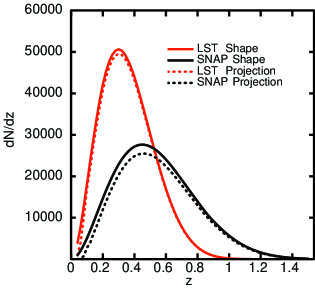
Figure 2: Cluster redshift distribution for LST and SNAP when $\rm{(S/N)_{min}}=5$. The solid lines correspond to the case when the shape noise dominates. The dotted lines show the cluster distribution when in addition to the shape noise we also include projection effects in the minimum detectable mass.

IV Fisher matrix calculations

In this section we use the Fisher information matrix to estimate how well WL cluster surveys can constrain the following parameters: $\Omega_{m}$, $\sigma_{8}$, $w_{0}$ and $w_{a}$. First we compute the number of clusters detectable by our fiducial surveys. Then we calculate the Fisher matrix considering Poisson noise and sample variance noise. Throughout this section we hold to the assumption that the intrinsic ellipticities of galaxies are the main noise source in the cluster measurements.

IV.1 Cluster abundances

As mentioned in section §II, the identification of the projected mass with the virial mass allows us to calculate the number of detectable clusters as an integral of the mass function$\,\frac{dN}{dV\,dM}$. The number of clusters per unit solid angle is

$$\frac{dN}{d\Omega}=\int_{0}^{\infty}dz\frac{dV}{dz\,d\Omega}\,\int_{M_{{\rm min}}(z)}^{\infty}d\ln{M}\,\frac{dN(M,z)}{dVd\ln{M}}\,.$$ (19)

Here dV is the comoving volume element and $\rm{M_{min}(z)}$ is the virial mass of a cluster still detectable at redshift $z$, obtained from equations (13) and (16) from section §III. The comoving number density of halos is given by: $\frac{dN}{dVd\ln{M}}\,d\ln{M}=\frac{\rho}{M}f(\nu)d\nu$, where $\rho$ is the comoving matter density and $f(\nu)$ is a semi-analytic dimensionless form of the mass function. $\nu=\frac{\delta_{sc}^{2}}{\sigma^{2}}$, $\delta_{sc}$ is the critical density for spherical collapse and $\sigma^{2}(M,z)$ is the linear density field variance, smoothed with a top-hat filter. $\sigma(M,z)$ is the only quantity in the mass function that depends on the dark energy equation of state through the growth factor:

$$\sigma(M,z)=D(z)\,\sigma(M,z=0)\,.$$

We assume a Sheth-Tormen $f(\nu)$ Sheth & Tormen (1999):

$$f_{ST}(\nu)=A\sqrt{\frac{a}{2\pi\nu}}\left[1+(a\nu)^{-p}\right]\exp(-a\nu/2)\,,$$

with $A=0.3222,a=0.707,p=0.3,\delta_{sc}=1.69$.

IV.2 The Fisher matrix

The Fisher matrix calculations were completed for cells corresponding to pairs of bins in redshift and filtered shear $\{z,\mbox{$\tilde{M}$}\}$. This choice of binning has two major benefits. Firstly, we use a directly measured quantity, the (filtered) shear $\tilde{M}$, rather than an inferred mass, to describe the data. Thus we can monitor how both the number of objects in a bin and their masses change with cosmology, in accordance with equations (13) and (19). Secondly, we retain information on the number vs $\tilde{M}$ i.e. we use the shape of the mass function. Most papers dealing with cluster Fisher matrix estimations wash away the information given by the shape of the mass function by integrating the mass function over mass above threshold. We considered 50 $\tilde{M}$-bins and 35 redshift bins, going from 0 to 2.

Ignoring the errors in redshift determinations (for both galaxies and clusters), bin counts are affected by 2 kinds of noise: Poisson noise and sample variance noise. The latter arises from the fact that the large scale structure of the universe correlates the number density of virialized objects in different volume elements. Hu & Kravtsov (2003) have studied the importance of sample variance noise relative to Poisson noise in cluster surveys . They concluded that sample variance can dominate Poisson noise for low-mass clusters, $M\leq\,4\times 10^{14}M_{\odot}/h$.

The Poisson Fisher matrix is defined as:

$$F_{\alpha\beta}=\sum_{i=1}^{I}N_{i,\alpha}\,N_{i,\beta}\frac{1}{N_{i}}\,,$$ (20)

where $N_{i,\alpha}=\partial N_{i}/\partial p_{\alpha}$ and $p_{\alpha},p_{\beta}$ can be any of the four parameters mentioned earlier. $N_{i}$ is the estimated number of clusters for bin $i$ and $I$ is the total number of bins.

To account for the correlations between bins, we follow Lima & Hu (2004) and employ an approximation of the Fisher matrix from the limiting cases of Poisson dominance and sample variance dominance:

$$F_{\alpha\beta}=\rm{N_{,\alpha}^{t}\,C^{-1}N_{,\beta}}+\frac{1}{2}\,\rm{Tr}[C^{-1}\,S_{,\alpha}\,C^{-1}\,S_{,\beta}]\,.$$ (21)

$\rm{N}$ is a vector of length $I$ whose elements are the $N_{i}$’s from above. $C$ is the covariance matrix (dimension $I\times I$), a sum of the shot noise and the sample covariance noise: $C=S+\mathcal{N}$. $\mathcal{N}$ is a diagonal matrix with $N_{i}$ on its diagonal. The sample covariance matrix is (e.g. Hu & Kravtsov (2003)):

$$S_{ij}=b_{i}b_{j}N_{i}N_{j}D_{i}D_{j}\int\frac{d^{3}k}{(2\pi)^{3}}W_{i}(\vec{k})W_{j}^{*}(\vec{k})P_{\rm{lin}}(k)\,.$$

Here $i$ and $j$ are bin indices, $P_{\rm{lin}}(k)$ is the linear power spectrum and $b$ is the linear bias as given by Sheth & Tormen (1999) :

$$b(M,z)=1+\frac{a\delta_{sc}^{2}/\sigma^{2}-1}{\delta_{sc}}+\frac{2p}{\delta_{sc}[1+(a\delta_{sc}^{2}/\sigma^{2})^{p}]}\,,$$

where $a$, $p$ and $\delta_{sc}$ have the same values as for the mass function. $D$ is the linear growth factor and $W_{i}(\vec{k})$ are the survey windows. As suggested in (Hu & Kravtsov, 2003), we considered the survey windows a series of concentric cylinders (redshift slices) at comoving distance $r_{i}$, of height $\delta r_{i}$ $(\delta r_{i}\ll r_{i})$, all subtending the same angle $\theta_{s}$. In Fourier space such windows have the expression:

$$W_{i}(\vec{k})=2\exp({ik_{\parallel}r_{i}})\,\frac{\sin({k_{\parallel}}\delta r_{i}/2)}{k_{\parallel}\delta r_{i}/2}\,\frac{J_{1}(k_{\perp}r_{i}\theta_{s})}{k_{\perp}r_{i}\theta_{s}}\,,$$

where $k_{\parallel}$ and $k_{\perp}$ are the components of $\vec{k}$, parallel and perpendicular to the line of sight and $J_{1}$ is the first order Bessel function.

IV.3 Results

To the cluster constraints we have added CMB constraints obtained for a Planck-type experiment with 65% sky coverage (Masahiro Takada, private communication). The temperature and polarization power spectra and the cross spectrum were computed using CMBFAST version 4.5.1. The Fisher matrix was initially calculated for 9 parameters: $\omega_{\rm cdm}$, $\omega_{b}$, $\Omega_{DE}$, $w_{0}$, $w_{a}$, $n$ (primordial power spectrum index), $A_{s}$ (amplitude of initial scalar fluctuations), $\alpha$ (primordial running index), and $\tau$ (optical depth at recombination). This 9-dimensional matrix was then projected into our 4-dimensional parameter space and the new matrix was added to the Fisher matrix given by equation (21). Two tables corresponding to $(S/N)_{\rm{min}}=5$ and $(S/N)_{\rm{min}}=10$ are shown below.

We first note that the constraints from the two experiments are remarkably similar. LST measures $\sigma_{8}$ slightly better than SNAP, while the opposite is true for $w_{a}$, the parameter describing the evolution of the dark energy equation of state. We expect this trend: due to its higher detection threshold, LST takes more information from the steep high-mass end of the mass function, where a variation in $\sigma_{8}$ is very acutely felt. On the other hand, SNAP can see higher redshift clusters and test a deeper survey volume than LST, so is more sensitive to the evolution of the dark energy equation of state.

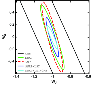
Figure 3: Poisson+sample variance constraints on $w_{0}$ and $w_{a}$ when $(S/N)_{\rm{min}}=5$: From outermost to innermost, CMB is black, SNAP is green, LST is red (dashed), SNAP+LST is blue and finally the cyan ellipse is obtained by combining SNAP+LST+CMB. The intrinsic ellipticities of galaxies are the dominant noise here and we have marginalized over $\Omega_{m}$ and $\sigma_{8}$.

The effect of sample variance on the dark-energy constraints is minimal, $\leq 15\%$ for the SNAP survey and $<5\%$ for LST. Adding CMB information brings down the constraints on all parameters, but especially on $w_{a}$, by $\approx 50\%$ for both instruments. This is further improved (by $40\%-50\%$) if we consider LST and SNAP as independent experiments (assuming they probe different survey volumes) and just sum their Fisher matrices. This can be seen best in figure 3, where we have plotted the constraints on the dark energy equation of state parameters for both telescopes when $(S/N)_{\rm{min}}=5$.

Finally we note that dark energy constraints depend strongly on choice of threshold $(S/N)_{\rm min}$. Doubling the detection threshold to 10 degrades the cosmological constraints by a factor $\sim 2$ for the SNAP$+$CMB case, or factors of $\sim 3$ for LST$+$CMB.

We conclude that both instruments have similar performances and that, at least for constraining dark energy, cluster counts are useful when combined with other experiments. Our results are far less optimistic than the predictions given by Wang, Khoury & Haiman (2004), but we shall defer comparisons with other papers to the last section.

$\rm{(S/N)_{\!min}=5}$	SNAP
	Poisson	Poisson+SV	Add CMB
$\Omega_{m}$	0.005	0.006	0.005
$\sigma_{8}$	0.006	0.007	0.006
$w_{0}$	0.078	0.087	0.069
$w_{a}$	0.304	0.348	0.197
	LST
$\Omega_{m}$	0.004	0.005	0.004
$\sigma_{8}$	0.004	0.004	0.004
$w_{0}$	0.076	0.077	0.062
$w_{a}$	0.373	0.380	0.182
	LST+SNAP
$\Omega_{m}$	0.003	0.003	0.003
$\sigma_{8}$	0.003	0.003	0.003
$w_{0}$	0.043	0.046	0.038
$w_{a}$	0.197	0.213	0.125

Table 1: 1-$\sigma$ constraints obtained for $(S/N)_{min}=5$, considering only the intrinsic ellipticity noise.

$\rm{(S/N)_{\!min}=10}$	SNAP
	Poisson	Poisson+SV	Add CMB
$\Omega_{m}$	0.014	0.014	0.012
$\sigma_{8}$	0.013	0.013	0.011
$w_{0}$	0.203	0.204	0.147
$w_{a}$	0.915	0.940	0.397
	LST
$\Omega_{m}$	0.015	0.015	0.013
$\sigma_{8}$	0.011	0.011	0.008
$w_{0}$	0.268	0.269	0.190
$w_{a}$	1.590	1.600	0.548
	LST+SNAP
$\Omega_{m}$	0.007	0.007	0.007
$\sigma_{8}$	0.006	0.006	0.005
$w_{0}$	0.121	0.123	0.092
$w_{a}$	0.644	0.661	0.268

Table 2: 1-$\sigma$ constraints obtained for $(S/N)_{min}=10$, considering only the intrinsic ellipticity noise.

V Large scale structure projections

It has been anticipated that WL cluster measurements will be substantially compromised by the so-called projection effects: the lensing signal could be produced by any structures along the line of sight, not just virialized clusters. This effect causes uncertainties in cluster mass determinations and consequently in cluster abundancies (e.g. Dodelson (2004) for a comprehensive discussion of errors on mass estimations and solutions to reduce them; see also Hoekstra (2001, 2003); Maturi et al. (2005)). Hennawi & Spergel (2004) study numerically the efficiency of locating clusters in shear maps and conclude that about 15% of the most significant peaks detected in noiseless WL maps do not have a collapsed halo with mass greater than $10^{13.5}M_{\odot}/h$ within a 3’ aperture; also see the related work of Hamana,Takada & Yoshida (2004).

The purpose of this section is to determine how important the large scale projections are for cluster counting and parameter constraints. We shall first consider the lensing signal of clusters with masses $\textit{b}elow$ the detection threshold computed in §III as the $\textit{o}nly$ source of noise for the projected mass measurement (i.e. we ignore completely the intrinsic shape noise of galaxies). We shall also regard the signal of these smaller clusters as wholly uncorrelated with the signal of detectable clusters employed for the estimates in §IV, presuming them to be at widely separated redshifts. Given these assumptions, we would like to establish the minimum detectable mass of a cluster at an arbitrary redshift $z_{d}$. We follow the steps of section §III to calculate the variance of the mass estimator $\tilde{M}$, replacing the intrinsic-ellipticity noise with the projection noise. We retain the weights derived in §III by optimizing the $S/N$ for the intrinsic-ellipticity noise. Although this is no longer an optimal filter, it allows us to compare the shape noise and the projection noise and to establish the redshift regime where each of them dominates.

V.1 The mass estimator

When the noise of the small structures along the line of sight dominates our measurement the contributions of different source-redshift bins are correlated, so we need to calculate the tangential shear power spectrum of these bins, as indicated by  (5). Since the convergence power spectrum is easier to estimate than the tangential shear spectrum, we reexpress the mass estimator in terms of convergence rather than shear:

$$\mbox{$\tilde{M}$}=\int d^{2}\theta\,\sum_{i}w_{\kappa}(\theta,z_{i})\kappa(\theta,z_{i})\,,$$ (22)

where we have considered directly the case of continuous annuli. The new convergence weights are linked to the old shear weights in the following manner (see for instance Schneider (1996)):

$$w_{\kappa}(x)=2\int_{x}^{\infty}dy\,\frac{w_{\gamma}(y)}{y}\,-w_{\gamma}(x)\,.$$ (23)

As already said, we take the same shear weights that optimize the shot noise filter and manipulating a little equation (23) we obtain for the convergence weights:

$$w_{\kappa}(\theta,z)=\left\{\begin{array}[]{ll}\frac{\mathcal{C}}{\frac{\sigma_{\gamma}^{2}}{n}}\left[\kappa(\theta,z)-\bar{\kappa}(\theta_{lim},z)\right]\,,\;\;\theta\leq\theta_{lim}\\ 0,\;\;\;\theta>\theta_{lim}\;,\end{array}\right.$$ (24)

with $\theta_{lim}$ defined in §III and the mean convergence inside a radius $\theta$, $\bar{\kappa}(\theta,z)=\frac{2}{\theta^{2}}\int_{0}^{\theta}dx\,x\,\kappa(x,z)$. Just like in §III, we shall use the convergence of a canonical cluster with an NFW profile density. $\mathcal{C}$ is the constant defined by equation (8).

We write the estimator defined by (22) in Fourier space and take its variance:

$${\rm Var}(\mbox{$\tilde{M}$})=\frac{1}{(2\pi)^{2}}\sum_{i,j}\int\,d^{2}l\,w_{\kappa}(\vec{l},z_{i})\,\mathcal{P}_{\rm{\kappa}}^{ij}(l)\,w_{\kappa}(\vec{l},z_{j})\,,$$ (25)

where we have used the definition of the convergence power spectrum:

$$\langle\kappa(\vec{l},z_{i})\,\kappa(\vec{l^{\prime}},z_{j})\rangle\equiv(2\pi)^{2}\,\mathcal{P}_{\kappa}^{ij}(l)\,\delta_{D}(\vec{l}-\vec{l^{\prime}})\,,$$

and the Fourier transform of the convergence weight:

$$w_{\kappa}(\vec{l},z)=2\pi\int_{0}^{\infty}d\theta\,\theta\,w_{\kappa}(\theta,z)\,J_{0}(l\,\theta)\,.$$

The power spectrum for bins $i,j$ is: (see for instance Takada & Jain (2004))

$$\mathcal{P}_{\rm{\kappa}}^{ij}(l)=\left(\frac{3}{2}\frac{H_{0}^{2}}{c^{2}}\Omega_{m}\right)^{2}\,\int_{0}^{\infty}dz_{p}\left|\frac{d\chi}{dz_{p}}\right|(1+z_{p})^{2}$$

$$\hskip 31.2982pt\times\;W_{i}(z_{p})W_{j}(z_{p})P_{\rm{\delta}}\left(\frac{l}{\chi(z_{p})},z_{p}\right)$$

$P_{\rm{\delta}}$ is the 3D matter power spectrum and $\chi$ is the comoving distance. The source weights are given by the expression:

$$W_{i}(z)=\frac{\int_{z_{i}}^{z_{i+1}}\,dz_{s}\mathcal{P}(z_{s})\,Z(z_{s},z)}{\int_{z_{i}}^{z_{i+1}}\,dz_{s}\mathcal{P}(z_{s})}\,.$$

In the limit of infinite number of redshift bins this simplifies to: $W_{i}(z)=Z(z_{i},z)\,.$

Combining all these ingredients and using  (24), the projection noise is thus defined:

$${\rm Var}(\mbox{$\tilde{M}$},z_{d})=\mathcal{C}^{2}\!\left(\frac{3}{2}\frac{H_{0}^{2}}{c^{2}}\Omega_{m}\right)^{2}$$

$$\hskip 14.22636pt\times\int d^{2}l\,\left\{d\theta\,\theta\left[\kappa_{\infty}(\theta,z_{d})-\bar{\kappa}_{\infty}(\theta_{lim},z_{d})\right]J_{0}(l\theta)\right\}^{2}$$

$$\hskip 14.79555pt\times\int_{0}^{\infty}dz_{p}\left|\frac{d\chi}{dz_{p}}\right|(1+z_{p})^{2}P_{\rm{\delta}}\left(\frac{l}{\chi(z_{p})},z_{p}\right)$$

$$\hskip 15.6491pt\times\left[\int_{0}^{\infty}dz_{s}\,Z(z_{s},z_{d})Z(z_{s},z_{p})\mathcal{P}(z_{s})\right]^{2}$$ (26)

The nonlinear matter power spectrum is computed using the halo model Smith et al. (2003): it is the sum of a quasi-linear term and a halo term. The quasi-linear term gives the power resulting from correlations of distinct halos and dominates on large scales. The halo term describes the correlations of particles within the same halo and dominates on small scales. At every $z_{p}$ (projection redshift), $P_{\rm{\delta}}$ is estimated as the power of the virialized structures with masses smaller than $M_{{\rm min}}(z)$ from section §III. Recall that halos above this mass are detected as clusters and are hence part of the signal, so do not contribute to the noise variance in the cluster-counting experiment.

V.2 Projection Noise vs. Ellipticity Noise

Equation (26) represents the projection noise, caused by the “unseen” small clusters that our featured surveys cannot detect, but which contribute nonetheless to the whole lensing signal. Solving again equation (16) with the variance given by (26) we find $M_{{\rm min}}^{\rm{proj}}(z)$ associated with this noise. In figure 1 we have plotted the minimum detectable mass corresponding to the shape noise (solid line) and to the projection noise (dotted line) for LST and SNAP when $(S/N)_{\rm{min}}$ is 5. We note that projection noise exceeds intrinsic-shape noise only for $z<0.07$ for LST, or slightly higher ($z<0.11$) for SNAP due to its lower shape-noise level. If $(S/N)_{\rm{min}}$=10, the crossover redshifts are 0.1 and 0.4, respectively.

There are 2 factors that decide the function $M_{\rm{min}}^{\rm{proj}}(z)$. Its shape is determined by the sources’ redshift distribution and its amplitude by the magnitude of the power spectrum that we integrate in (26). To understand why the projection noise is so high at small redshifts compared to the shape noise, we have to look at the way $S/N$ scales with $D_{d}$ (the lens-observer angular diameter distance) in each case. At small redshifts, the signal gets weak, because the shear gets weak. When the shape noise dominates, $S/N$ does not have a dependence on $D_{d}$ because the signal scales with $D_{d}$ the same way the noise does. This is not true for projection noise, where the noise and the signal scale differently, so $S/N\rightarrow 0$ as $z\rightarrow 0$ at fixed mass. A cluster produces a maximum lensing signal if it lies halfway between the source and the observer: $M_{\rm{min}}^{\rm{proj}}$ is minimal at the redshifts obeying this condition. For LST, $\langle z\rangle$ is 1, so the minimum occurs around 0.5. For SNAP it occurs at redshifts around 0.7, since $\langle z\rangle$ is 1.5 in this case. At higher redshifts LST has fewer sources than SNAP, so there $M_{\rm{min}}^{\rm{proj}}$ is higher for LST than for SNAP.

$M_{\rm{min}}^{\rm{proj}}$ is even more sensitive to the choice of the detection threshold than $M_{\rm{min}}^{\rm{shape}}$. In the case of shape noise, the variance of the mass estimator does not depend on $(S/N)_{\rm{min}}$, as one can see from equation (15). $(S/N)_{\rm{min}}$ impacts $M_{\rm{min}}^{\rm{shape}}$ only when we solve (16). In the case of projection noise, the variance itself depends on $(S/N)_{\rm{min}}$ through the power spectrum in equation (26). For every projection redshift, we have excluded from the total matter power spectrum the clusters with masses bigger than $M_{\rm{min}}^{\rm{shape}}$ corresponding to that redshift, because they are individually identifiable as clusters and can be removed from the noise background. Therefore, the remaining noise spectrum is stronger when $(S/N)_{\rm{min}}=10$ than when $(S/N)_{\rm{min}}=5$. In the same vein, $M_{\rm{min}}^{\rm{proj}}$ is greater for LST than for SNAP, because $M_{\rm{min}}^{\rm{shape}}$ is greater for LST than for SNAP. The importance of $(S/N)_{\rm{min}}$ is further propagated when we solve equation (16) for the variance given by (26). This is the reason why the difference between $M_{\rm{min}}^{\rm{proj}}$ obtained for $(S/N)_{\rm{min}}=5$ and $M_{\rm{min}}^{\rm{proj}}$ for $(S/N)_{\rm{min}}=10$ is greater than the difference between $M_{\rm{min}}^{\rm{shape}}$ corresponding to the same detection thresholds of 5 and 10.

In order to see the role of the projection noise in the cosmological parameter constraints, we have added the shape-noise critical mass and the projected-noise critical mass in quadrature and repeated the calculations from §IV. And just like in §IV, we took the variation with cosmology of the new total critical mass into account. Figure 2 shows the number of detectable clusters per unit redshift as a function of redshift when we consider only the shape noise (solid line) and both the shape and projection noises (dashed line). The total number of clusters does not decrease significantly ($\leq 10\%$) when the projection noise is included, if $(S/N)_{\rm{min}}=5$. There is negligible change to the derived cosmological constraints.

Raising the threshold to $10\sigma$ can cut the number of detectable clusters more severely, particularly for SNAP, where it eliminates 60% of detections. The effect upon derived parameter constraints remains small, however, if we combine the cluster surveys with either the CMB or with each other. Figure 4 shows the constraints on $w_{0}$ and $w_{a}$ obtained for SNAP first for ellipticity noise only and then when projections are included.

If the projection noise were to become a significant contributor to the error budget, one could construct an estimator that maximizes the signal-to-noise in the presence of both shape noise and projection noise Dodelson (2004); Maturi et al. (2005).

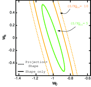
Figure 4: SNAP constraints on $w_{0}$ and $w_{a}$: the orange (outer) solid ellipse is for $(S/N)_{\rm{min}}=10$ and shape noise only, the green (inner) solid ellipse is for $(S/N)_{\rm{min}}=5$ and shape noise only. The dotted ellipses are obtained for $(S/N)_{\rm{min}}=5$ and when we add the projection noise to the shape noise. These are all Poisson+sample variance errors and we have marginalized over $\Omega_{m}$ and $\sigma_{8}$.

$\rm{(S/N)_{\!min}=5}$	SNAP
	Poisson	Poisson+SV	Add CMB
$\Omega_{m}$	0.006	0.006	0.006
$\sigma_{8}$	0.006	0.007	0.006
$w_{0}$	0.082	0.090	0.072
$w_{a}$	0.315	0.355	0.203
	LST
$\Omega_{m}$	0.005	0.005	0.005
$\sigma_{8}$	0.004	0.004	0.004
$w_{0}$	0.077	0.078	0.063
$w_{a}$	0.380	0.386	0.185
	LST+SNAP
$\Omega_{m}$	0.003	0.003	0.003
$\sigma_{8}$	0.003	0.003	0.003
$w_{0}$	0.044	0.047	0.038
$w_{a}$	0.201	0.216	0.126

Table 3: 1-$\sigma$ constraints obtained for $(S/N)_{min}=5$ when we add the projection noise to the intrinsic ellipticity noise.

VI Discussion and Conclusions

In this paper we have tried to determine how useful WL-detected clusters are for constraining cosmology. We focus our attention on the matter density parameter ($\Omega_{m}$), the power spectrum normalization ($\sigma_{8}$) and the time-evolving dark energy equation of state ($w_{0},w_{a}$), assuming a flat universe.

There are a few important features in our Fisher matrix analysis that distinguish it from previous work. We compute the Fisher matrix using as an observable the directly measured quantity, the filtered shear $\tilde{M}$. Assuming some density profile for the detected lenses, their measured shear can be converted to a virial mass. However, this conversion depends on the cosmology. In different cosmologies, different masses correspond to the same measured shear. Our Fisher matrix takes this fact into account. We have also employed the shape of the mass function, by keeping track of the $\tilde{M}$ of the objects in bins rather than merely counting clusters above a threshold. A third distinction of our analysis is the halo-model calculation of the noise variance due to uncorrelated projections along the line of sight. As noted above, this is shown to cause little loss of cosmological information in most circumstances.

When we apply our formalism to canonical ground (LST) and space (SNAP) WL surveys, we find the two are nearly equivalent. The lower cluster-mass threshold afforded by the deeper sample of source galaxies in space provides a 15-fold increase in the sky density of detected clusters, which compensates for the smaller survey solid angle that we assume for the SNAP survey. Both surveys produce quite interesting dark-energy constraints, and improve significantly when combined with CMB constraints. Combining the LST and SNAP surveys results in constraints significantly stronger than either alone.

Comparison with previous forecasts for WL cluster surveys is complicated by the extreme sensitivity to the assumed noise level and detection threshold of the survey—this behavior is of course generically true of cluster-counting experiments.

Our results are less encouraging than some other forecasts in the literature: for a detection threshold of 5 and considering only the intrinsic ellipticities of galaxies, LST could detect about 21500 clusters. The calculated LST errors on cosmological parameters are: $\Delta\Omega_{m}=0.005$, $\Delta\sigma_{8}=0.004$, $\Delta w_{0}=0.08$, $\Delta w_{a}=0.38$, if we take into account both the Poisson and sample variance noises. SNAP yields rather similar constraints.

These values obtained for the dark energy equation of state are a few times higher than found by Wang, Khoury & Haiman (2004): $\Delta w_{0}=0.05$ and $\Delta w_{a}=0.09$. These authors analyze an LST-type experiment, using a Gaussian filter for the shear signal, as proposed by Hamana,Takada & Yoshida (2004). Such a difference in our results is partly (but not completely) explained by the assumed parameters of their survey. The angular concentration of galaxies is 65 galaxies/$\rm{arcmin}^{2}$, the survey area is 18000$\rm{deg}^{2}$ and $\sigma_{\gamma}$ is 0.15, more optimistic than our corresponding values of 30 galaxies/$\rm{arcmin}^{2}$, 15000$\rm{deg}^{2}$ and 0.3. Additionally, they take $(S/N)_{\rm{min}}=4.5$. They estimate about 200000 clusters are detectable, $10\times$ higher than our nominal estimate. If we assume their input values, our optimal filter yields about 700000 clusters, demonstrating the advantage of an optimal filter.

The last issue that we discussed is that of the projection contamination, considered the sword of Damocles for WL measurements. From the beginning we make a crucial approximation: we identified the projected mass of clusters with their virial mass. This need not be true on a cluster-by-cluster basis, just in the sense that the mass functions have similar amplitude and dependence upon cosmological parameters. With this assumption—which needs to be verified numerically—about the effect of local structure on projected-mass estimates, we can next treat the projection of unrelated structures along the line of sight as a noise source, not a bias.

WL cluster measurements are subject to two major sources of noise: the intrinsic ellipticities of galaxies (shape noise) and these large scale projections. We find that, even when we use an overdensity-detection filter optimized for pure shape noise, that the projection noise is dominant only for lenses at $z_{d}\lesssim 0.1$, and has little effect upon the derived dark-energy constraints in most applications of our canonical ground (LST) and space (SNAP) WL cluster surveys.

Let us stress again that all these numbers are extremely sensitive to the detection threshold and the noise levels that we impose. If $(S/N)_{\rm{min}}=10$, the number of detectable clusters goes down by a factor of 10 in the case of shape noise only and by more than a factor of 18 when we also account for projections. Then the errors on the dark energy equation of state parameters are as much as tripled. If the noise has Gaussian statistics, as we would expect for shape noise, then the $5\sigma$ threshold will suffice to keep false positives to an unimportant level. The projection noise will not, however, be Gaussian, so further investigation is required to determine whether the $5\sigma$ threshold offers enough suppression. The numerical study of Hennawi & Spergel (2004) suggests this is the case, as their $4.5\sigma$ threshold results in a false-positive contamination of only 25%. Recall that this work considers any object not associated with a virialized halo to be a false positive, whereas we assert that counting unvirialized objects is a valid cosmological test, so this 25% “contamination” still carries cosmological information.

We conclude, therefore, that counting of WL-detected clusters can be a powerful constraint on cosmology with either space- or ground-based surveys. While projection effects make it difficult to establish a one-to-one correspondence between WL-derived masses and virial masses, there is no real need to make such a correspondence in order to infer cosmological parameters from WL data. Indeed it is precisely the ability to go directly from $N$-body simulations to WL-derived masses that makes WL cluster counting an attractive alternative to optical, X-ray, or SZ cluster counting. Our Fisher analysis incorporates the cosmological dependence of the conversion from shear to mass units, plus the effect of sample variance and projection noise, and we show that none of these are barriers to strong dark-energy constraints.

References

- Henry & Arnaud (1991) J. P. Henry and K. A. Arnaud, Astrophys. J. 372, 410 (1991).
- Henry (1997) J. P. Henry, Astrophys. J. 489, L1 (1997).
- Wang & Steinhardt (1998) L. Wang and P. J. Steinhardt, Astrophys. J. 508, 483 (1998).
- Kitayama & Suto (1997) T. Kitayama and Y. Suto, Astrophys. J. 490, 557 (1997).
- Bahcall & Fan (1998) N. A. Bahcall and X. Fan, Astrophys. J. 504, 1 (1998).
- Levine,Schulz & White (2002) E. S. Levine, A. E. Schultz and M. White, Astrophys. J. 577, 569 (2002).
- Eke,Cole & Frenk (1996) V. R. Eke, S. Cole and C. S. Frenk, MNRAS 282, 263 (1996).
- Holder,Haiman & Mohr (2001) G. P. Holder, Z. Haiman and J. J. Mohr, Astrophys. J. 560, L111 (2001).
- Weller,Battye & Kneissl (2002) J. Weller, R. A. Battye and R. Kneissl, Phys. Rev. Lett. 88, 1301 (2002).
- Battye & Weller (2003) R. A. Battye and J. Weller, Phys. Rev. D 68, 083506 (2003).
- Haiman,Mohr & Holder (2001) Z. Haiman, J. J. Mohr and G. P. Holder, Astrophys. J. 553, 545 (2001).
- Majumdar & Mohr (2003) S. Majumdar and J. J. Mohr, Astrophys. J. 585, 603 (2003).
- Majumdar & Mohr (2004) S. Majumdar and J. J. Mohr, Astrophys. J. 613, 41 (2004).
- Bahcall et al (2003a) N. A.Bahcall, T. A. Mckay, J. Annis et al, ApJS 148 243 (2003).
- Bahcall et al (2003b) N. A. Bahcall, F. Dong, P. Bode et al, ApJ. 585, 182 (2003).
- Bahcall et al (2003c) N. A. Bahcall, F. Dong, L. Hao et al, ApJ. 599, 814 (2003).
- Gladders (2000) M. D. Gladders, Bulletin of the Am. As. Soc. 32, 1499 (2000).
- Gladders & Yee (2005) M. D. Gladders and H. K. C. Yee, ApJS 157, 1 (2005).
- Lima & Hu (2004) M. Lima and W. Hu, Phys. Rev. D 70, 043504 (2004).
- Hu & Kravtsov (2003) W. Hu and A. V. Kravtsov, Astrophys. J. 584, 702 (2003).
- Hennawi & Spergel (2004) J. F. Hennawi and D. N. Spergel, Astrophys. J. 624, 59 (2005).
- Hamana,Takada & Yoshida (2004) T. Hamana, M. Takada and N. Yoshida, MNRAS 350, 893 (2004).
- Croft & Metzler (2000) R. A. C. Croft and C. A. Metzler, Astrophys. J. 545, 561 (2000).
- (24) http://snap.lbl.gov
- (25) http://lsst.org
- Spergel et al. (2003) D. N. Spergel, L. Verde, H. V. Peiris, E. Komatsu, M.R. Nolta et al., ApJS 148 175S (2003).
- Press & Schechter (1974) W. Press and P. Schechter, Astrophys. J. 187, 425 (1974).
- Sheth & Tormen (1999) R. K. Sheth and G. Tormen, MNRAS 308, 119 (1999).
- Jenkins et al (2001) A. Jenkins, C. S. Frenk, S. D. M. White, J. M. Colberg, S. Cole, A. E. Evrard, H. M. P. Couchman, N. Yoshida, MNRAS 321, 372 (2001).
- Warren et al (2005) M. S. Warren, K. Abazajian, D. E. Holz, L. Teodoro, astro-ph/0506395 (2005).
- Weinberg & Kamionkowski (2003) N. N. Weinberg and M. Kamionkowski, MNRAS 341, 251 (2003).
- Dodelson (2003) S. Dodelson, equation 10.25 from Modern Cosmology, Academic Press (2003).
- Bernstein & Jarvis (2002) G. M. Bernstein and M. Jarvis, Astrophys. J. 123, 583 (2002).
- Bernstein (2006) G. M. Bernstein, in preparation (2006).
- Smail et al. (1995) I. Smail, D. W. Hogg, L. Yan, J.G. Cohen, Astrophys. J. 449, L105 (1995).
- Bartelmann & Schneider (1999) M. Bartelmann and P. Schneider, Astron. Astrophys. 345, 17 (1999).
- Bartelmann (1996) M. Bartelmann, Astron. Astrophys. 313, 697 (1996).
- Wright & Brainerd (2000) C. O. Wright and T. G. Brainerd, Astrophys. J. 534, 34 (2000).
- Navarro,Frenk & White (1996) J. F. Navarro, C. S. Frenk and S. D. M. White, Astrophys. J. 490, 493 (1997).
- Wang, Khoury & Haiman (2004) S. Wang, J. Khoury, Z. Haiman et al., Phys. Rev. D 70, 123008 (2004).
- Dodelson (2004) S.Dodelson, Phys. Rev. D 70, 023008 (2004).
- Hoekstra (2001) H. Hoekstra, Astron. Astrophys. 370, 743 (2001).
- Hoekstra (2003) H. Hoekstra, MNRAS 339, 1155 (2003).
- Maturi et al. (2005) Maturi, M., Meneghetti, M., Bartelmann, M., Dolag, K., & Moscardini, L., Astron. Astrophys. 442, 851 (2005).
- Schneider (1996) P. Schneider, MNRAS 283, 837 (1996)
- Takada & Jain (2004) M. Takada and B. Jain, MNRAS 348, 897 (2004).
- Smith et al. (2003) R.E. Smith, J.A. Peacock, A. Jenkins, S.D.M. White, C.S. Frenk, F.R. Pearce, P.A. Thomas, G. Efstathiou and H.M.P. Couchman, MNRAS 341, 1311 (2003).