Elemental abundances in the atmosphere of clump giants.

Abstract

Aims. The aim of this paper is to provide the fundamental parameters and abundances for a large sample of local clump giants with a high accuracy. This study is a part of a big project, where the vertical distribution of the stars in the Galactic disc and the chemical and dymamical evolution of the Galaxy are being investigated.

Methods. The selection of clump stars for the sample group was made applying a color -absolute magnitude window to nearby Hipparcos stars. The effective temperatures were estimated by the line depth ratio method. The surface gravities ($\log\mathrm{g}$) were determined by two methods (the first one was the method based on the ionization balance of iron and the second one was the method based on fitting of the wings of Ca i 6162.17 Å line). The abundances of carbon and nitrogen were obtained from molecular synthetic spectrum, the Mg and Na abundances were derived using the non-LTE approximation. The “classical” models of stellar evolution without atomic diffusion and rotation-induced mixing were employed.

Results. The atmospheric parameters (${T_{\rm eff}}$, $\log\mathrm{g}$, [Fe/H], $\mathrm{V_{t}}$) and Li, C, N, O, Na, Mg, Si, Ca and Ni abundances in 177 clump giants of the Galactic disc were determined. The underabundance of carbon, overabundance of nitrogen and “normal” abundance of oxygen were detected. A small sodium overabundance was found. A possibility of a selection of the clump giants based on their chemical composition and the evolutionary tracks was explored.

Conclusions. The theoretical predictions based on the classical stellar evolution models are in good agreement with the observed surface variations of the carbon and nitrogen just after the first dredge-up episode. The giants show the same behavior of the dependencies of O, Mg, Ca, Si ($\alpha$-elements) and Ni (iron-peak element) abundances vs. [Fe/H] as dwarfs do. This allows one to use such abundance ratios to study the chemical and dynamical evolution of the Galaxy.

1 Introduction

Low-mass stars (i.e., below $\sim$ 2.3 $M_{\odot}$) climb the red giant branch (hereafter RGB) with a degenerate He core whose mass increases until it reaches a critical value of about 0.45 M_⊙ at the top of the RGB. At this point, helium ignites in a series of flashes removing this degeneracy. The star then becomes a “clump” giant which undergoes the central He burning. All the low-mass stars have similar core masses at the beginning of He burning, and hence the similar luminosities. Due to this fact, the red giants at this evolutionary stage exhibit a specific feature in the color - magnitude diagram (CMD), called the “clump”. According to evolutionary tracks and in agreement with the observation of open clusters, all giants older than about 1 Gyr fall in the clump (Girardi gir99 (1999)).

Clump giants are especially interesting from two aspects. Their intrinsic brightness combined with the numerous and sharp features of their spectra makes them good tracers for the galactic kinematics and chemistry. They are also very useful in clarification of the advanced evolutionary stages of the low mass stars. Until now, the comprehensive investigation of the large sample of these stars has not been carried out yet.

This work is a part of our study of the Galactic disc surface mass density (Siebert et al. siebet03 (2003), Bienaymé et al. bienet06 (2006)) of the properties of both thin and thick discs, and the abundance trends in the solar neighbourhood (Soubiran et al. 2003, Mishenina et al. mskk04 (2004), Soubiran & Girard 2005). In this part of the project, the local clump giants observed with high spectral resolution and high signal-to-noise ratio (S/N) serve as reference stars. Here we take the opportunity to provide the strong observational constraints for the theory of stellar evolution. As a matter of fact, the chemical composition of the clump giant atmospheres reflects both the chemical composition of the prestellar matter and nucleosynthesis and mixing processes inside the stars. Therefore, for successful Galactic studies we need to know the abundances of which chemical elements are not affected by the mixing processes. On the other hand, we can use the elements with abundances affected by the mixing processes to distinguish different stages of the stellar evolution, especially the clump phase.

While investigating the clump giants, we faced the problem of their selection , since this region of the CMD is also occupied by the stars of the ascending giant branch. The differentiation between the first-ascending RGB stars and the “clump” stars is rather complicated. Even for open cluster stars, it is very difficult to establish with the good level of certainty, which stars from the group under investigation are the real clump ones (Pasquini et al., paset04 (2004)). We can solve the problem of the correct selection using the extended observational data on the clump giants, selected with photometric criteria. However, is it possible to identify the clump giants based on additional criteria, including the data about their chemical composition?

When the star moves towards the RGB, the superficial convection zone deepens and the nuclearly processed material penetrates into the atmosphere changing of its chemical composition. During this so-called first dredge-up phase, the surface abundances of Li, C, N, and Na, together with the ¹²C/¹³C ratio, are being altered. The effect depends both on the stellar mass and metallicity (see Charbonnel 1994). Typically, the surface abundance of carbon decreases by $\sim$ 0.1-0.2 dex and that of nitrogen increases by 0.3 dex or more (Iben iben91 (1991)).

Despite a large dispersion, the abundances of CNO elements and their isotopes observed previously in the giants of the solar metallicity (Lambert, Ries lamrie81 (1981); Kj$\ae$rgaard et al. kijgus82 (1982)) were found to be in a good agreement with theoretical predictions (Iben iben91 (1991)). We reinvestigate this problem with a larger sample of stars which have been observed with higher quality.

For giants and supergiants of the solar metallicity the sodium overabundance has been found in many studies (Cayrel de Strobel et al. cayet70 (1970), Korotin & Mishenina kormish99 (1999), Boyarchuk et al. boyet01 (2001), Andrievsky et al. andet02 (2002)). As has been shown in some papers (Mashonkina et al. maset93 (1993), Korotin & Mishenina kormish99 (1999)) the Na overabundance cannot only be explained by deviations from LTE. In this paper, we look into this problem using recent theoretical considerations and track calculations. The aim of this paper is to provide the fundamental parameters and abundances for a large sample of local clump giants, determined with a high accuracy and to use these data to 1) probe the vertical distribution of the stars in Galactic disc, 2) investigate the Galactic chemical evolution, and 3) explore the possibility to select the clump giants based on their elemental abundances.

In Sect. 2 we described the photometric selection criteria for the clump giants and the detail of our spectroscopic observations. In Sect. 3, the determination of the atmospheric parameters is presented. In Sect. 4, the chemical abundances are determined. In Sect. 5, we discussed the behaviour of each element in our sample with metallicity. In Sect. 6 we provided the analysis of the signs of the first dredge-up in stars under current study.

2 Selection of the stars and observations

The clump stars analysed in this paper were selected using a colour-absolute magnitude window applied to nearby Hipparcos stars. Stars were selected from the Hipparcos catalogue according to the following criteria:

$$\pi\geq 10\,\rm{mas}$$

$$\delta_{\rm{ICRS}}\geq-20\deg$$

$$0.8\leq B-V\leq 1.2$$

$$0\leq M_{\rm V}\leq 1.6$$

where $\pi$ is the Hipparcos parallax and $\delta_{\rm{ICRS}}$ the declination. The Johnson $B-V$ colour was transformed from the $Tycho$2 $B_{\rm T}-V_{\rm T}$ colour applying Eq. 1.3.20 from ESA, (1997):

$$B-V=0.850\,(B{\rm{}_{T}}-V{\rm{}_{T}})$$

The absolute magnitude $M_{\rm{V}}$ was computed using the $V$ magnitude transformed from the Hipparcos $H_{\rm p}$ magnitude to the Johnson system with the equation calibrated by Harmanec (har98 (1998)).

Among the selected nearly 400 giants, about a half of them were observed: the first priority group contained stars, for which radial velocities were not determined, and their [Fe/H] were not accurate or were old. The known spectroscopic binaries were excluded.

The list was completed with a few clump stars having distances in the range of 100-200 pc, for which we were expecting the low metallicity. Most of the clump stars with $B-V$ between 0.75 and 0.8, even lacking previously published metallicities, were also included in the list and observed. Finally, we have included six $Tycho$-2 stars that are distant clump stars located at about 500 pc from the Galactic plane toward the North Galactic Pole. They were previously identified from the low S/N spectra (Bienaymé et al. bienet06 (2006)).

The spectra of the studied stars were obtained using the facilities of the 1.93 m telescope of the Haute-Provence Observatoire (France) equipped with échelle-spectrograph ELODIE. The resolving power was 42000, the region of the wavelengths was 4400 - 6800 Å, the signal-to-noise ratio was about 130-230 (at 5500 Å). The initial processing of the spectra (image extraction, cosmic particles removal, flatfielding etc) was carried out following to Katz et al. (katzet98 (1998)). Further processing of the spectra (continuum level location, measurement of the equivalent widths etc) was performed using the software package DECH20 (Galazutdinov gal92 (1992)). The equivalent width were measured using the Gaussian fitting.

In Fig. 1 we have shown the comparison of our EWs measured in the spectrum of HD 180711 with those reported by Boyarchuk et al. (boyet96 (1996)). In the paper of Boyarchuk et al. (boyet96 (1996)) the spectra of program star were obtained using the 2.6 m telescope of the Crimean astrophysical observatory (Ukraine) with coudé – échelle spectrograph. The reciprocal dispersion of those spectra was 3 Å/mm. An agreement between two independent EW systems appears to be good, as one can see in Fig. 1. $\Delta$EW = EW(our) – EW(Boyarchuk) = 0.23$\pm$4.5 mÅ.

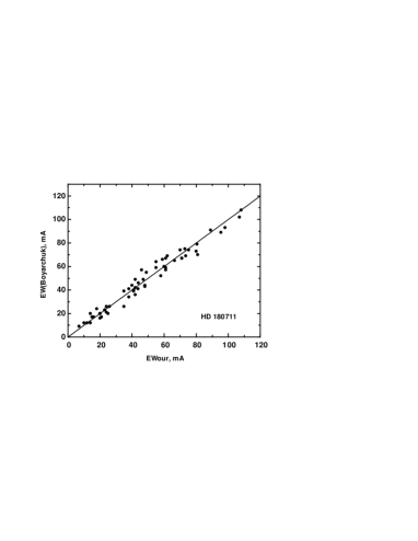
Figure 1: Comparison between EWs measured from the spectrum of HD 180711 and those from Boyarchuk et al. (1996). Upper panel: EWs from Boyarchuk et al.(1996); lower panel: our determinations.

The basic characteristics of studied stars are given in the Table A. The spectral classes $Sp$, magnitudes $V$(Simbad) were taken from SIMBAD database and magnitude $V$(Hipparcos) transformed fron the Hipparcos $H_{p}$ to the Johnson system, parallaxes $\pi$ from Hipparcos catalogue (ESA 1997), M_V were calculated. The 6 fainter stars of the sample are not part of the Hipparcos catalogue. Their spectral type come from SIMBAD. The V magnitudes have been extracted from the General Catalogue of Photometric Data by Mermilliod et al (1997). Absolute magnitudes Mv have been estimated from the TGMET software.

3 Atmospheric parameters

3.1 Effective temperature ${T_{\rm eff}}$

The temperatures were determined with the very high level of accuracy ($\sigma=10-15$ K) using the line depth ratios The spectral lines of high and low excitation potentials respond differently to the change in effective temperature ($T_{\rm eff}$). Therefore, the ratio of their depths (or equivalent widths) is a very sensitive temperature indicator. This technique allows one to determine ${T_{\rm eff}}$  with an exceptional level of accuracy. The method used is based on the ratio of the central depths of two lines having very different functional ${T_{\rm eff}}$dependences. This method is independent of the interstellar reddening and only marginally dependent on individual characteristics of the stars, such as rotation, microturbulence and metallicity. NLTE effects will most likely affect ratios of high- and low-excitation line strenthgs, and ratios between different chemical elements. Perhaps, these effects and also those of varying individual stellar chemical abundance can be reduced by the statistics of a large number of different line ratios. The zero-point is well established and is based on a large number of independent measurements from the literature; it would be unlikely that the error on the zero-point is larger than 20–50 K.

We used a set of 100 line ratio – ${T_{\rm eff}}$  relations obtained in Kovtyukh et al. (kovtet06 (2006)), with the mean random error of a single calibration being 65–95 K (45–50 K in most cases and 90–95 K in the least accurate cases). The use of $\sim$70–100 calibrations per spectrum reduces the uncertainty to 5–25 (1 $\sigma$) K. This precision indicates that these 100 calibrations are weekly sensitive to non-LTE effects, metallicity, surface gravity, micro- and macroturbulence, rotation and other individual stellar parameters. These relations have been calibrated with the reference stars in common with Gray & Brown (gray01 (2001)) – 21 stars, $\sigma$=27 K, Blackwell & Lynas-Gray (BLG98 (1998)) – 18 stars, $\sigma$= 81 K, Alonso, Arribas & Martínez-Roger (AAM99 (1999)) – 14 stars, $\sigma$=47 K, Strassmeier & Schordan (ss00 (2000)) – 20 stars, $\sigma$=71 K and Soubiran, Katz & Cayrel (soubet98 (1998)) – 103 stars, $\sigma$=106 K (see Fig.2) For the majority of stars, we obtained an internal error smaller than 20 K.

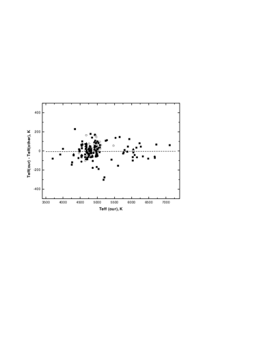
Figure 2: Comparison between the temperatures derived in the present work and those derived by Gray & Brown (2001) – open squares, Blackwell & Lynas-Gray (1998) – solid circles, Alonso, Arribas & Martínez-Roger (1999) – solid triangles, Strassmeier & Schordan (2000) – open circles, Soubiran, Katz & Cayrel (1998) – solid squares.

After the accurate effective temperatures have been determined, the other atmospheric parameters were found iteratively.

3.2 Surface gravity $\log\mathrm{g}$, microturbulent velocity $\mathrm{V_{t}}$ and metallicity [Fe/H]

Because clump giants have similar luminosity but, different initial masses, their gravities cannot be correctly determined using their parallaxes and mass data. These $\log\mathrm{g}$ values are affected by $\pm$ 0.3dex if the stellar mass is based on a assumption of mass of 2.2M_⊙. We used two following methods of spectroscopic determinations of the gravity $\log\mathrm{g}$: 1) using the iron ionization equilibrium assumption, where the average iron abundance determined from Fe i lines and Fe ii lines must be identical, and 2) from the wing fitting of Ca i 6162 Å  line. For the method of the ionization equilibrium, we have used iron lines with EW $<$ 120 mÅ; the wing profiles for such lines practically do not depend on damping constants, but they are sensitive to microturbulent velocity $\mathrm{V_{t}}$  and metallicity [Fe/H]. Therefore, we take adopted ${T_{\rm eff}}$  and then we obtain the parameters ($\log\mathrm{g}$, $\mathrm{V_{t}}$ and [Fe/H]) iteratively. Two or three steps were enough to get a good convergence.

The second method is motivated by the fact that the Ca i line is strong in giants, and therefore its wing profile is sensitive to the gas pressure in a stellar atmosphere, and therefore to the surface gravity. The use of the Ca i triplet lines (6102, 6122, 6162 Å) as indicator of surface gravity was proposed for dwarfs and subgiants by Edvardsson (edv88 (1988)) and analyzed by Cayrel et al. (cayet96 (1996)). Cayrel et al. (1996) have explored a possible influence of errors on the profiles of these lines. They found that a change of 10$\%$ of the damping constants has a negligible influence, a change of 15$\%$ becomes more or less detectable. The effective temperatures were also varied by 100 K and no alteration of profiles was detected. NLTE effects are important in the core of the line but negligible in the wings. Recently Affer et al. (alfet05 (2005)) used this method for K dwarfs and subgiants. We have applied this method to giants to assess our gravity determination in case of iron ionization equilibrium. The Ca i 6162 Å  line which was recommended by Katz et al. (katzet03 (2003)) as a best luminosity indicator among the triplet lines, was used. We have estimated the influence of atmospheric parameter uncertainties on accuracy of the gravity determination. The Ca i wings are not sensitive to the microturbulent velocity $\mathrm{V_{t}}$. A change by 30 K in ${T_{\rm eff}}$  brings the errors in $\log\mathrm{g}$ about 0.05 - 0.10 (for ${T_{\rm eff}}$= 5000 K and 4500 K, respectively). To determine the calcium abundance value, we used weaker Ca I lines which are presumed to be less affected by the damping and the microturbulent velocity.

The departures from LTE in the computation of the wing profiles for these lines are negligible for dwarfs and subgiants (Cayrel et al. cayet96 (1996)), but in the case of giants it may elevate the level of uncertainty in $\log\mathrm{g}$ up to 0.2 dex. The total error of the $\log\mathrm{g}$ determination for giants is about 0.2-0.3 dex. An example of the line wing fitting for HD 180711 is given in Fig. 3. The values of $\log\mathrm{g}$  obtained by two methods, are given in Table A. The mean difference $\Delta$ ($\log\mathrm{g}$(Ca)-$\log\mathrm{g}$(IE)) is -0.01 $\sigma=\pm 0.09$ The results of these two methods applications are in good agreement. The value of surface gravity for each star was obtained by keeping condition of the ionization equilibrium between the Fe I and Fe II species and these values were used for abundance determination.

The value of microturbulent velocity $\mathrm{V_{t}}$ is determined by the standard method from a condition of independence of the iron abundances determined from the given line of Fe i upon its equivalent width EW. The accuracy of $\mathrm{V_{t}}$ determination is $\Delta$ $\mathrm{V_{t}}$=$\pm$ 0.2 km s^-1.

The [Fe/H] metallicity is obtained from the abundance determined from Fe i lines. (In this paper we use the customary spectroscopic notation [X/Y]=log₁₀(N_X/N_Y)_star – log₁₀(N_X/N_Y)_⊙)

In Table A we give the mean ${T_{\rm eff}}$, the number of calibrations used ($N$), the errors of the mean $\sigma$, $\log\mathrm{g}$, $\mathrm{V_{t}}$, metallicities [Fe/H]_I and [Fe/H]_II were determined from Fe i and Fe ii lines, correspondingly.

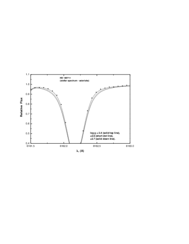
Figure 3: Derivation of $\log\mathrm{g}$ from the Ca i 6162 Å  profile for HD 180711.

4 Determination of chemical abundances

We employ the grid of stellar atmospheres from Kurucz (1993) to compute abundances of Li, C, N, O, Na, Mg,Si, Ca and Ni. The choice of the model was made using the standard interpolation on ${T_{\rm eff}}$  and $\log\mathrm{g}$. The abundance analysis of Si, Ca, Ni and Fe has been done in the LTE approximation (Kurucz’s WIDTH9 code) using the measured equivalent widths of these elements’ lines and the solar oscillator strengths (Kovtyukh & Andrievsky kovand99 (1999)). Abundances of Fe, Si, Ca, Ni were derived from a differential analysis relatively to the Sun’s data (see discussion in Mishenina et al. 2004). In Table A the relative-to-solar Fe, Si, Ca, Ni abundances and individual errors are given.

4.1 The Li abundance

The Li abundances in program stars were obtained by fitting synthetic spectra to the observational profiles. We used STARSP LTE spectral synthesis code developed by Tsymbal (tsy96 (1996)). Considering a wide range of temperatures and metallicities of our sample stars, the special effort was put into a compilation of a full list of atomic and molecular lines close to the ⁷Li 6707 Å line (Mishenina & Tsymbal, mistsy97 (1997)). In Fig. 4, the comparison was made of the observed and the calculated spectra of HD 90633, for different lithium abundances log A(Li) = 1.0, 1.85, and 2.1, where log A(X) = 12 + log(N_X/N_H). The derived values of log A(Li)$>$ 0.5 dex are given for 24 stars in Table A. We consider the lithium abundance of about 0.5 dex as a lower limit of the reliable determination. The comparison of our results with values found in the literature (Brown et al. broet89 (1989)) shows a good agreement $\Delta$ logA(Li)Brown - logA(Li)our = –0.01 $\pm 0.13$ (for 8 common stars).

4.2 CNO abundances

The abundances of carbon, nitrogen and oxygen are determined by the method of synthetic spectrum using the STARSP code (Tsymbal, tsy96 (1996)). The spectrum of a molecule C₂ at the 5630 Å (head of a band C₂ (0,1) of the Svan system d${}^{3}\Pi_{g}$ – a${}^{3}\Pi_{u}$ was used to derive the carbon abundance. The nitrogen abundance was determined from the spectrum of a molecule CN at 6330 Å  and 6470 Å  (red system A${}^{2}\Pi$ – X${}^{2}\Sigma$, heads of bands CN (5,1) and (6,2)). The wavelengths and parameters of molecular lines (including log gf) were taken from Kurucz (1993), and they were corrected using the technique proposed by Kuznetsova & Shavrina (kuzsha96 (1996)). For these spectral regions, the contribution from blended lines of other systems of a molecule C₂, molecule CN and (NH, OH, CH, MgH and SiH) was estimated. The lines from our list were compared to the lines from solar spectrum, using the atmosphere model from the Kurucz’s grid. The contribution from the blended lines in the solar spectrum appears to be insignificant (except for lines of a molecule CN in the regions of a molecule C₂ and line [OI] 6300.3 Å ). For the region of a molecule C₂ and [OI] 6300.3 Å  line, the CN lines were included in the final line list. The calculation was carried out with the following dissociation potentials D₀ (C₂) = 6.15 eV and D₀ (CN) = 7.76 eV. In Fig. 5, a comparison between synthetic spectrum and observed one near 5630 Å  is shown. In Table A the abundances of carbon, nitrogen, oxygen are given with the scale $log$ A(H) = 12. Below we use the values of relative to solar and iron abundances ([C,N,O/Fe]) The solar C,N,O abundances are determined from fitting the synthetic and solar spectra. As solar spectra we used those of the Moon and asteroids that obtained with spectrograph ELODIE. The adopted solar values of log log A(C), log A(N), log A(O) are the following: 8.55, 7.97, 8.70, respectively.

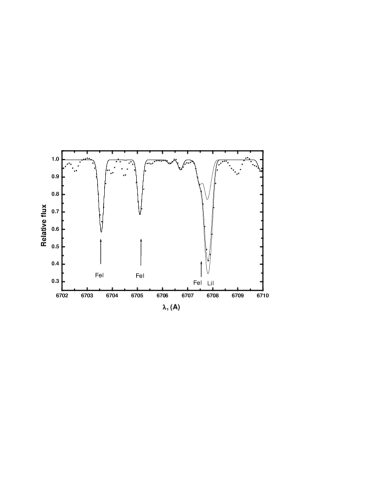
Figure 4: Comparison between the observed specrum for HD 90633 and synthetic one with the Li abundances logA(Li) = 1.0, 1.85, and 2.1.

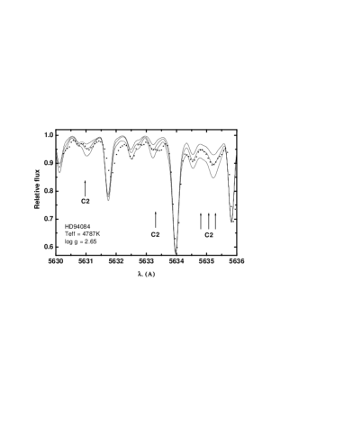
Figure 5: Comparison between the observed specrum for HD 94084 and synthetic one with the C abundances logA(C) = 8.36, 8.46, and 8.56.

4.3 NLTE abundances of magnesium and sodium

In the spectra of cool giants the lines of sodium and magnesium are strong enough (EW$>$ 200 mÅ), therefore one can expect a significant deviation from LTE. For determination of the abundances of Na and Mg we used NLTE approximation. Four lines of Na i and 9 lines of Mg i were considered.

NLTE abundances of Mg and Na were determined with the help of a modified version of the MULTI code (Carlsson car86 (1986)) described in Korotin et al. (1999a ) and Korotin et al. (1999b ). In such a modified version, in particular, additional opacity sources from ATLAS9 code (Kurucz kur93 (1993)) were included. This was done in order to calculate the continuum opacity more precisely, and to take into account the absorption by a great number of spectral lines (especially within the region of the near UV). It allows one to calculate more accurately the intensity distribution in the region 900–1500 Å. In turn, this significantly affects the determination of the radiative rates of bound – free transitions. A simultaneous solution of the radiative transfer and statistical equilibrium equations has been performed in the approximation of complete frequency redistribution for all the lines. All the NLTE calculations were also based on the Kurucz’s grid of atmospheric models.

4.4 Parameters of sodium and magnesium atoms

The model of sodium atom as described by Sakhibullin (sah87 (1987)), has been modified (see Korotin & Mishenina kormish99 (1999)). It consists of 27 levels of Na i and the ground level of Na ii. We considered the radiative transitions between the first 20 levels of Na i and the ground level of Na ii. Transitions between the remaining levels were used only in the equations of particle number conservation. Finally, 46 $bound-bound$ and 20 $bound-free$ transitions were included in the linearization procedure. For 34 transitions the radiative rates were fixed.

Figure 6: NLTE profile fitting for HD 162076 (for the line Na i 5683Å) and LTE profile (dashed line).

Figure 7: Same as Fig. 6 but for the lines Na i 6164, 6160.

We employed the model of magnesium atom consisting of 97 levels: 84 levels of Mg i, 12 levels of Mg ii and a ground state of Mg iii. Within the described system of the magnesium atom levels, we considered the radiative transitions between the first 59 levels of Mg i and ground level of Mg ii. Transitions between the rest levels were not taken into account and they were used only in the equations of particle number conservation. For detail see Mishenina et al., mskk04 (2004).

The difference between synthetic and observed spectra becomes visible if the sodium and magnesium abundances are changed by about 0.05 dex. The difference between sodium and magnesium abundances derived under the LTE assumption and for NLTE case is within an interval of 0.10-0.15 dex. As an example, for better comparison we have shown the LTE line profile (dashed line)in Figs. 6, 7, 8, 9.

Figure 8: Same as Fig. 6 but for the lines Mg i 4703.

Figure 9: Same as Fig. 6 but for the lines Mg i 5173, 5184.

In Table A NLTE abundances of Na and Mg are given in the scale where logA (H) = 12.

4.5 Abundance determination errors

The metallicities [Fe/H] for the giants have been determined. These determination were based on the iron abundance value derived from Fe i lines. For this purpose, we used from 100 to 170 lines depending on the temperature of the star: for the cooler stars the number of iron lines was lower. The typical line-to-line scatter for Fe i is 0.11 dex s.d. The abundances of silicon, calcium and nickel have been determined from 12 to 22 lines of Si i, 8 to 10 lines of Ca i and 15 to 20 lines of Ni i. Typical standard deviations of the abundances derived from a single line of these elements are 0.12, 0.14, and 0.10 respectively.

Several factors may influence the abundance determination. Among them are: 1) the accuracy of the model parameters, 2) the equivalent width measurements, 3) the quality of the synthetic spectrum adjustment, and 4) internal errors of the method used. Concerning the last factor, one can notice that somewhat different abundance results can be obtained if one uses the LTE or Non-LTE approximations, 1D-, 2D- or 3D atmosphere models. There are also uncertainties in atomic constants. The use of the differential method minimizes these determination errors. Uncertainties that are attributed to observed spectrum are the following. A change in equivalent width of 2mÅ corresponds to a change in abundance of about 0.03 – 0.06 dex for Fe i, Si i, Ca i, Ni i. The fitting procedure between synthetic and observed spectra in the case of C₂ lines produces uncertainty of about 0.02 dex. In other cases (N, Na, Mg) it is about 0.05 dex. The value of total uncertainty due to the choice of the stellar parameters is shown in Table 1. The atmospheric parameters were changed by $\Delta$ Teff = +100 K, $\Delta$ $\log\mathrm{g}$= +0.2, $\Delta$ [Fe/H] = –0.25 for [Fe/H] $<$ 0 and $\Delta$ [Fe/H] = +0.1 for [Fe/H]$>$0, $\Delta$ Vt= +0.2 km s^-1.

As one can see from Table 1, the total uncertainty reaches 0.18 – 0.24 dex for iron abundance determined from Fe ii species and 0.10 – 0.12 dex in the case of the Fe i species. For C, N, O abundances, such uncertainties are: 0.13 – 0.23, 0.09 – 0.13, 0.09 – 0.21 respectively. In the case of carbon, the maximal error takes place for the cooler stars. For oxygen the uncertainty is caused by the choice of the model metallicity for metal-deficient stars. For Na, Mg, Si abundances, the total error is about 0.08 – 0.11 and for Ca and Ni it is about 0.11 – 0.16. The microturbulence uncertaintly supplies the largest uncertaintly to the Fe i iron abundance.

Table 1: Abundance determination errors. Parameter variation and corresponding uncertainty in abundance determination ($\Delta$ Teff = +100 K, $\Delta$ $\log\mathrm{g}$= +0.2, $\Delta$ [Fe/H] = –0.25 for [Fe/H] $<$ 0 and $\Delta$ [Fe/H] = +0.1 for [Fe/H]$>$0, $\Delta$ Vt= +0.2 km s^-1)

. Element $\Delta$${T_{\rm eff}}$ $\Delta$$\log\mathrm{g}$ $\Delta$$\mathrm{[Fe/H]}$ $\Delta$$\mathrm{V_{t}}$ $\Delta$ tot HD161178 4789/2.2/-0.24/1.3 FeI 0.06 0.01 –0.03 –0.10 0.12 FeII –0.10 0.08 –0.19 –0.08 0.24 LiI 0.14 0.00 0.02 –0.01 0.14 CI –0.12 0.05 0.03 0.00 0.13 NI 0.08 0.03 –0.10 0.00 0.13 OI 0.02 0.09 –0.19 0.00 0.21 NaI 0.08 –0.03 0.02 –0.07 0.11 MgI 0.07 –0.02 –0.04 –0.06 0.10 SiI –0.02 0.03 –0.08 –0.04 0.10 CaI 0.11 0.00 0.05 –0.07 0.14 NiI 0.05 0.03 –0.06 –0.08 0.12 HD17361 4646/2.5/0.12/1.5 FeI 0.03 0.03 0.03 –0.09 0.10 FeII –0.11 0.17 0.08 –0.05 0.22 LiI 0.16 –0.01 0.00 0.00 0.16 CI –0.13 0.15 –0.01 0.00 0.20 NI 0.03 0.07 0.05 0.00 0.09 OI –0.04 0.13 0.05 0.00 0.14 NaI 0.09 0.00 –0.01 –0.07 0.11 MgI 0.05 0.01 0.03 –0.06 0.08 SiI –0.05 0.09 0.04 –0.05 0.12 CaI 0.09 –0.01 –0.01 –0.07 0.11 NiI 0.03 0.07 0.05 –0.11 0.14 HD27697 4975/2.65/0.11/1.4 FeI 0.07 0.00 0.00 –0.08 0.11 FeII –0.07 0.09 –0.13 –0.06 0.18 LiI 0.12 –0.01 0.07 –0.01 0.14 CI –0.10 0.07 –0.19 0.00 0.23 NI 0.08 0.03 0.06 0.00 0.10 OI 0.02 0.09 0.00 0.00 0.09 NaI 0.07 –0.02 0.00 –0.05 0.09 MgI 0.06 –0.02 0.03 –0.03 0.08 SiI –0.01 0.03 –0.05 –0.04 0.07 CaI 0.09 –0.01 0.02 –0.06 0.11 NiI 0.05 0.02 –0.05 –0.14 0.16

5 Abundance trends with metallicity

5.1 The C, N, O abundance

The abundance ratios [C/Fe], [N/Fe], [O/Fe] for each star in our set are plotted against [Fe/H] in Figs. 10, 11 and  13. For the whole sample of giants, the average values of the abundances of these elements are the following: $<[C/Fe]>=-0.23\pm 0.08$; $<[O/Fe]>=0.08\pm 0.16$; $<[N/Fe]>=0.25\pm 0.09$, for the stars of metallicity [Fe/H]$>$–0.3 they are: $<[C/Fe]>=-0.24\pm 0.07$; $<[O/Fe]>=0.04\pm 0.12$; $<[N/Fe]>=0.24\pm 0.08$. and for stars near solar metallicity –0.01 $<$[Fe/H]$<$ 0.01 they are: $<[C/Fe]>=-0.28\pm 0.05$; $<[O/Fe]>=0.02\pm 0.08$; $<[N/Fe]>=0.21\pm 0.07$. These averaged abundance ratios agree well with evolutionary model predictions of Iben (iben91 (1991)), who showed that stars should have decreased carbon and increased nitrogen abundances in their atmospheres.

Thus, our data (see Fig. 10) exhibit a clear anticorrelation between [C/Fe] and [Fe/H]. In Fig. 12 we compare our determinations (open circles) of the carbon abundance with those of Lambert & Ries lamrie81 (1981) (filled circles), Kj$\ae$rgaard & Gustafsson kijgus82 (1982) (asterisks) for all stars. The mean values obtained in these mentioned works are: $<[C/Fe]>=-0.22\pm 0.21$ (Lambert & Ries lamrie81 (1981)), $<[C/Fe]>=-0.31\pm 0.30$ (Kj$\ae$rgaard & Gustafsson kijgus82 (1982)). They are within the error limits of determinations with our value $<[C/Fe]>=-0.23\pm 0.08$, but in our case we have smaller scatter. The dependence of [C/Fe] on [Fe/H] (see Fig. 12) is clearly observed only for our clmp giant sample. Whether is it a feature of the clump stars? Probably, not. The same behaviour of [C/Fe] versus [Fe/H] was discovered in the disc dwarfs (Bensby & Feltzing benfel06 (2006); Reddy et al. reddet06 (2006)), but the avarege values of [C/Fe] are different for dwarfs and for giants. Therefore, we can conclude that observed trend is not a peculiar feature of the clump giants, since it reflects the general tendency of the C abundance decreasing with [Fe/H] increasing. We have detected it because our [C/Fe] are obtained with a smaller scatter comparing to others similar works.

We have found some (not distinctive) dependence between [N/Fe] and [Fe/H] (see Fig. 11), but quite large scatter for our nitrogen data prevents us from making a definitive conclusion. An analysis of the C and N abundances

within the frameworks of the evolutionary models is presented in Sec. 6.

The abundance of oxygen increases with the metallicity decrease (see Fig. 13). This behaviour is similar to $\alpha$-element behaviour in the dwarf stars. This confirms the well-known fact that the relative-to-iron abundance of the $\alpha$-elements decreases when the metallicity increases. This is connected with the growing contribution from the SNe I stars to the iron enrichment. Obviously, the determined oxygen abundance in giants can be used in an investigation of Galactic evolution.

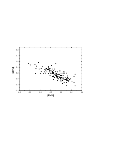
Figure 10: Carbon abundance [C/Fe] vs. [Fe/H].

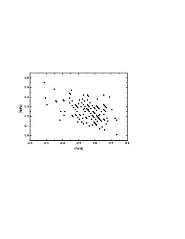
Figure 11: Nitrogen abundance [N/Fe] vs. [Fe/H].

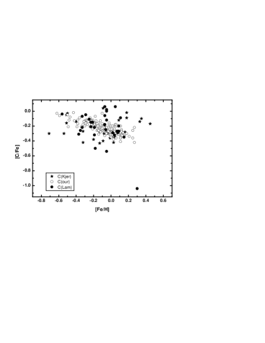
Figure 12: Comparison of our carbon abundances (open circles) and those of Kj$\ae$rgaard et al. 1982 (asterisks) and Lambert & Ries 1981 (filled circles).

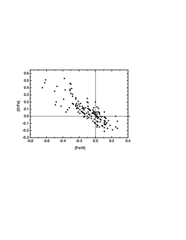
Figure 13: Oxygen abundance [O/Fe] vs. [Fe/H].

5.2 The Na abundance

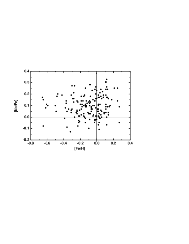
Figure 14: Sodium abundance [Na/Fe] vs. [Fe/H].

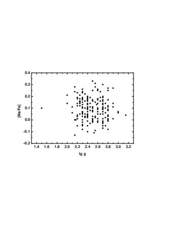
Figure 15: Sodium abundance [Na/Fe] vs. $\log\mathrm{g}$.

Figure 16: Sodium abundance [Na/Fe] vs. nitrogen abundance [N/Fe]

We found a small Na overabundance about 0.1 dex (see Fig. 14), and we also established that there is no visible dependence of [Na/Fe] upon $\log\mathrm{g}$  (see Fig. 15). Some overabundance of sodium can be the sign of the NeNa cycle opration. Nevertheless, an absence any dependence between [Na/Fe] and $\log\mathrm{g}$  does not support this supposition. From the other hand, this can be result of a restricted region of the $\log\mathrm{g}$  we considered. Additionally there is a correlation between [Na/Fe] and [N/Fe] (see Fig. 16). We notice that the behaviour of [Na/Fe] vs [Fe/H] is not similar for giants and for dwarfs (Soubiran & Girard sougir05 (2005)). We will consider the sodium abundance below in Sec. 6.

5.3 The $\alpha$-element and Ni abundances

The behaviour of Mg, Ca, Si ($\alpha$-elements) and Ni (iron-peak element) (see Figs. 17, 18, 19, 20) abundances vs. [Fe/H] in giants is the same as in dwarfs (Soubiran & Girard sougir05 (2005)). It allows one to use abundances of these elements to study the chemical and dynamical evolution of the Galaxy.

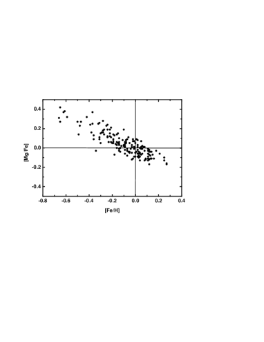
Figure 17: Magnesium abundance [Mg/Fe] vs. [Fe/H]

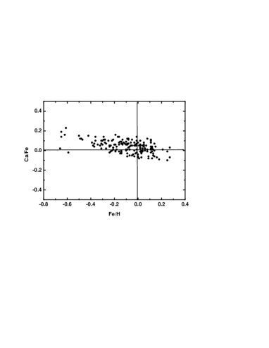
Figure 18: Calcium abundance [Ca/Fe] vs. [Fe/H]

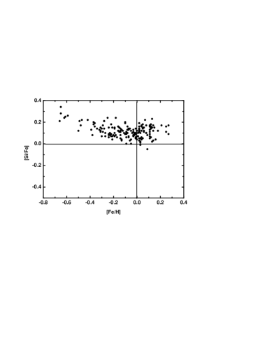
Figure 19: Silicon abundance [Si/Fe] vs. [Fe/H]

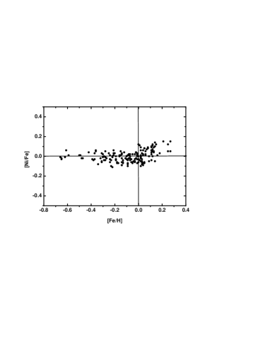
Figure 20: Nickel abundance [Ni/Fe] vs. [Fe/H].

6 Abundance variations due to the first dredge-up

Due to surface abundance modifications during the first dredge-up episode, clump giants do not exhibit the chemical pattern that they inherited at their birth. In this section we compare our data with first dredge-up theoretical predictions.

6.1 Stellar models

We computed evolution models from the pre-main sequence up to the AGB phase for stars with initial masses of 1.0, 1.5, 2.0, 2.5 and 3.0 M_⊙ and for three values of [Fe/H], i.e., –0.293, 0, and +0.252 using the code STAREVOL (i.e., Siess et al. 2000, Palacios et al. 2006). These are “classical” models, i.e., they do not take into account atomic diffusion and rotation-induced mixing. The nuclear reaction rates are those of NACRE (Angulo et al. 1999). For the radiative opacities, we use the OPAL tables above 8000 K (Iglesias & Rogers 1996) and at lower temperatures the atomic and molecular opacities of Alexander & Fergusson (1994). The conductive opacities are computed from a modified version of the Iben (1975) fit to the Hubbard & Lampe (1969) tables for non-relativistic electrons and from Itoh et al.(1983) and Mitake et al.(1984) for relativistic electrons. The equation of state is described in detail in Siess et al.(2000) and accounts for the non-ideal effects due to Coulomb interactions and pressure ionization. The standard mixing length theory is used to model convection th $\alpha_{\rm MLT}=1.75$ calibrated for the solar case. Neither overshooting, nor undershooting is considered for convection. The atmosphere is treated in the gray approximation and integrated up to an optical depth $\tau\simeq 5\times 10^{-3}$. Mass loss is considered during the whole evolution and follow the Reimer’s (1975) empirical relation.

6.2 Comparison with theoretical predictions

In Figs. 21, 22 and 23 we show the corresponding evolutionary tracks together with the positions of the sample stars in the HR diagram. As expected, the objects appear to be slightly more massive in the average when one moves to the higher metallicity.

Also shown in these figures are the predictions for the surface abundance variations of C, N and Na as a function of effective temperatures along the RGB together with the corresponding observational data. Stars with [Fe/H] below –0.15 are compared with the [Fe/H]=–0.293 tracks, those with [Fe/H] between –0.15 and +0.12 are compared with the [Fe/H]=0 tracks, and the more metallic ones with the [Fe/H]=+0.252 tracks. As can be seen the region of the clump in the evolutionary tracks overlaps the region where the first dredge-up ceases.

Our finding on the nitrogen abundance is in good agreement with the prediction of the canonical theory of evolution for first dredge-up phase.

In the case of carbon, we show two sets of tracks for the two more metallic subsamples. The full lines are those assuming an initial [C/Fe] equal to solar, while the dotted lines are obtained by simply shifting the previous ones by –0.15 and –0.20 dex respectively. These quantities correspond to the values of the upper envelope of [C/Fe] at the corresponding [Fe/H] (see Fig. 10). Again, the models explain well the observational pattern.

Regarding sodium the observed dispersion is higher than the theoretical one. Numerous overabundances are observed, especially for the more metal-rich subsample. This cannot be attributed to an extra-mixing process, because any additional processing of the envelope of the giant would also lead to further changes in the C and N abundances which are not observed in our sample. One possibility to remove part of the discrepancy could lie in the rates that intervene in the NeNa cycle. For the reaction that forms sodium, ²²Ne(p,$\gamma)^{23}$Na, the new rate calculated by Hale et al. (2001) is slightly smaller (for the central temperature of the models on the main sequence, i.e., below $\sim$ 20 million degrees) than the NACRE prescription used in the present computations. It would thus not favour stronger dredge-up of sodium. On the other hand the present uncertainty of the ²³Na(p,$\gamma)^{24}$Mg and ²³Na(p,$\alpha)^{20}$Ne reactions is still large (Hale et al. 2004). There also exist a possibility that the initial sodium abundance was higher for some stars. The disc dwarfs show some dispersion of the Na abundance and this is confirmed, for example, by Mishenina et al.(2003) and Edvardsson et al. (1993) (especially for [Fe/H]$>$ 0).

In the central regions of the main sequence stars, ¹⁶O is partially converted into ¹⁴N. However the convective envelope hardly reaches the O-depleted region during the first dredge-up for the mass range considered here (see for example Fig. 1 of Charbonnel 1994). As a consequence surface O variations are not expected in our sample stars (Fig. 24). We just observe in our sample of giants an O/Fe versus Fe/H variation (Fig. 13) exactly similar to the variation observed with dwarfs (see Figures 4 and 10 in Soubiran, Girard, 2004).

Figure 21: Comparison of the theoretical tracks and predictions for surface abundance variations with observations. Position of our target stars with [Fe/H]$<$–0.15 in the H-R diagram

Figure 22: Same as Fig. 21 for [Fe/H]=0. Top right panel: the full lines are those assuming an initial [C/Fe] equal to solar, while the dotted lines are obtained by simply shifting the previous ones by –0.15.

Figure 23: Same as Fig. 22 for [Fe/H]=0.252 and [C/Fe]=–0.20.

Figure 24: Predictions for surface abundance variations of O during the first dredge-up for the [Fe/H]=0 models and comparison with the observations

6.3 The Li abundance

According to the theory, the surface Li abundance decreases with respect to its value at the end of the main sequence (MS) by a factor from 30 to 60, depending on the stellar mass and metallicity (Iben 1991). Starting from the present interstellar medium abundance of log N(Li) = 3.3 we thus expect after the first dredge up the Li values that lie around 1.5 as shown in Fig. 25. Let’s insist on the fact that these are “classical” predictions which do not take into account the effect of non-standard transport processes such as those induced by rotation and which are thus not able to explain the Li patterns observed in low-mass main sequence stars (Charbonnel & Talon 2005; see the review by Deliyannis et al. 2000) By such, we have the right to expect for our giants lower values of lithium, as proves to be true by observations (Brown et al. broet89 (1989), Mallik mal99 (1999)).

The observed Li abundances versus the effective temperatures for the giants studied here are depicted in Fig. 25.

In the case of low-mass stars (M${}_{star}<$2.2–2.5 M_⊙, HD 8733, 15453, 42341, 46374, 90633, 117304, 136138, 139254, 148604, 171994, 192836) that undergo some extra-mixing at the RGB bump (Charbonnel et al. 1998, Charbonnel & Balachandran 2000), the fact that we see some Li certainly indicates that these objects are RGB stars which have not yet reached the bump. Otherwise their Li would have been destroyed.

In the case of more massive stars which do not undergo this extra-mixing because they do not go through the bump, Li should be consistent with standard post dredge-up value predicted by the models.

Most likely, the Li abundance cannot be used as the criterion to segregate the clump giants from RGB giants.

Figure 25: Li abundance logA(Li) vs. ${T_{\rm eff}}$  for our sample stars compared with the theoretical predictions for the tracks at [Fe/H]=0. The line with the strongest Li depletion corresponds to the 1.0M_⊙ model

6.4 Determination of the evolutionary status

The stars considered in this study have been selected as clump stars according to photometric criteria. Nevertheless, our sample could be contaminated by ascending giant branch stars which cohabit with clump stars in the considered region of the CMD (see Figs. 21, 22 and 23). It would thus be interesting to perform more subtle separation of the clump giants from the whole sample of the stars.

We aimed to do this selection by comparing the abundances of individual stars with theoretical predictions of stellar evolution models. This is however a very difficult task since the clump overlaps the region where the first dredge-up ceases in the evolutionary tracks. Despite this difficulty we checked the status of each sample stars individually following the procedure described below.

We first attributed a mass and evolutionary status to each object by comparing its position in the HRD with the theoretical tracks. The values of obtained masses for our target stars are given in the Table A1. Again, the stars with [Fe/H] below –0.15 are compared with the [Fe/H]=–0.293 models, those with [Fe/H] between –0.15 and +0.12 are compared with the [Fe/H]=0 models, and the more metallic ones with the [Fe/H]=+0.252 ones. From this first iteration 125 of our sample stars were identified as possible RHB or clump stars, 4 as subgiants, 38 as probable RGBs, and 2 are likely AGB stars.

Then we checked for each star whether its nitrogen abundance was compatible with the model predictions for the corresponding stellar mass attributed previously. The carbon abundance was used only as a cross-check because of the variation it presents as a function of metallicity (see §5.1). Among the 125 possible RGB/clump stars, 15 objects have no N determination and 32 objects appear to still undergoing the first dredge-up dilution as indicated by their [N/Fe] and effective temperature. For the others we made the following distinctions : (i) 38 stars are found to have completed their first dredge-up but present N abundances slightly lower (by 0.05 to 0.2 dex) than predicted values for the corresponding stellar mass. 3 stars have N overabundances by $\sim$ 0.2 dex. We consider however that these slight discrepancies are not significant because of the observational errorbars on the effective temperature and on the abundance determination. Moreover, part of the small discrepancy can be accounted for by the fact that not all the stars have the exact metallicity of the theoretical tracks they are compared with. (ii) 16 giants have a N abundance in good agreement with the post-dredge predictions for the given stellar mass. Both the (i) and (ii) stars would be preferentially identified as RGB stars according to their effective temperature, although they are still good clump candidates. (iii) 21 stars could be selected as clump giants according to both their N abundance in good agreement with the post-dredge predictions and their effective temperature.

We have thus reliably selected 21 clump giants plus 54 clump candidates, and about 100 usual giants that show all the signs of first dredge-up. Unfortunately, we have to state that there exists some uncertainty in the separation of the clump giants if we rely only on the evolutionary tracks and elemental abundances that are sensitive to the stellar evolution.

An important conclusion of the present study is that the theoretical predictions of the classical models do account well for the observed surface variations of both carbon and nitrogen during the first dredge-up episode.

However, it would be note that the considered analysis and the result depend on accuracy of determination of chemical composition and the used theoretical preconditions.

7 Conclusions

We have performed the detailed analysis of the atmospheric parameters and the abundances of some elements in 177 giant stars.

The stars analysed in this study have been selected as clump stars according to the photometric criteria. We have estimated the possibillity to define the evolutionary status of these giants on the basis of evolutionary tracks and their measured element abundances that are modified during the stellar evolution. We reliably selected 21 clump giants, about 54 clump candidates and about 100 usual giants that show all the signs of first dredge-up.

The determined C, N and Na abundances in our program stars reflect the CNO- and NaNe cycle operation in the giant stars.

The O, Mg, Ca, Si ($\alpha$-elements) and Ni (iron-peak element) abundances in giants show trends similar to those observed in dwarfs. This allows one to use these abundances to study the chemical and dynamical evolution of the Galaxy.

Acknowledgements. T.M. and V.K. want to thank the Observatoire Astronomique de l’Université Louis Pasteur de Strasbourg for kind hospitality. We also thank the referee, Prof. B. Edvardsson, for very useful and fruitful comments and suggestions on the manuscript. The work was made within the framework of the French - Ukrainian project ”Dnipro” - ”Egide”.

Appendix A

[x]rlccrrr The basic characteristics of studied stars
Star Sp $V$ (Simbad) $V$(Hipparcos)$\pi$ (0.001)$M_{V}$ Masses
Continued.
Star Sp $V$ (Simbad) $V$(Hipparcos)$\pi$ (0.001)$M_{V}$ Masses
2910 K0III 5.347 5.38 12.69 0.432 2.2
4188 K0III 4.775 4.77 15.54 0.331 2.5
4482 G8II 5.515 5.51 12.45 0.646 2.5
5395G8III-IV 4.632 4.62 15.48 0.202 2.0
6319 K2III: 6.193 6.20 10.01 0.696 1.7
6482 K0III 6.101 6.09 10.58 0.780 2.0
7106K0,5III 4.523 4.51 20.11 0.563 2.0
7578 K1III 6.050 6.04 10.36 0.647 2.0
8207 K0III 4.875 4.87 16.68 0.550 2.5
8599 G8III 6.167 6.17 12.17 1.176 1.2
8733 K0 6.450 6.44 10.71 1.262 2.0
9408 G9III 4.692 4.68 15.96 0.303 2.0
10975 K0III 5.947 5.94 10.57 0.705 1.5
11559 K0III 4.621 4.61 17.11 0.471 2.7
11749 K0III 5.698 5.69 10.18 0.257 2.0
11949 K0IV 5.712 5.70 13.25 0.861 1.0
15453 K2III 6.098 6.09 11.4 0.913 1.7
15755 K0III 5.846 5.84 12.54 0.813 1.5
15779 G3III 5.364 5.36 12.27 0.414 2.5
16247 K0III: 5.819 5.81 11.18 0.549 1.0
16400 G5III: 5.656 5.65 10.29 0.334 2.5
17361K1,5III 4.510 4.52 18.06 0.292 2.0
18885 G6III: 5.834 5.84 11.55 0.693 2.2
19270 K3III 5.648 5.64 10.21 0.240 2.5
19787 K2III 4.350 4.35 19.44 0.405 2.7
19845 G9III 5.921 5.93 10.47 0.684 2.5
20791G8.5III 5.690 5.70 11.23 0.630 2.5
25602K0III-IV 6.320 6.31 10.21 0.894 1.2
25604 K0III 4.354 4.36 18.04 0.207 2.7
26546 K0III 6.091 6.09 11.42 0.939 2.0
26659 G8III 5.477 5.47 10.74 0.397 3.0
26755 K1III 5.727 5.72 12.38 0.679 1.5
27348 G8III 4.933 4.93 14.42 0.423 3.0
27371 G8III 3.654 3.65 21.17 –0.043 3.0
27697 G8III 3.746 3.77 21.29 0.070 3.0
28292 K2III 4.971 4.96 16.78 0.458 1.0
28305 K0III 3.540 3.53 21.04 –0.185 3.0
28307 G7III 3.847 3.84 20.66 0.100 3.0
30557 G9III 5.642 5.64 10.16 0.287 2.5
31444G6/G8III 5.726 5.71 11.3 0.719 2.2
33419 K0III 6.118 6.11 10.37 0.735 2.0
33618K2III-IV 6.147 6.15 10.61 0.738 1.5
34200 G5 6.384 6.39 8.5 0.749 2.5
34559 G8III 4.956 4.96 15.83 0.652 2.5
35369 G8III 4.144 4.13 18.71 0.167 3.0
37638 G5III: 6.168 6.17 10.26 0.957 2.5
39070 G8III 5.490 5.49 10.51 0.364 3.0
39910 K2III: 4.874 5.87 10.71 –0.497 3.0
40020 K2III 5.891 5.89 10.62 0.536 2.2
40801 K0III 6.092 6.08 12.47 1.106 1.0
42341 K2III 5.563 5.56 15.53 1.023 2.0
43023 G8III 5.835 5.83 10.36 0.603 2.5
45415 G9III 5.553 5.55 11.15 0.360 2.2
46374 K2III: 5.562 5.57 12.75 0.598 2.0
46758 G5 7.156 7.15 5.15 0.411 2.2
47138G8/K0III 5.704 5.71 11.79 0.838 2.5
47366 K1III: 6.117 6.11 11.75 1.044 1.2
48432 K0III 5.349 5.34 15.69 0.941 1.5
50904 G5 6.539 6.53 7.02 0.444 2.5
53329 G8IV 5.557 5.55 10.68 0.399 2.0
54810 K0III 4.920 4.91 15.45 0.378 1.5
55280 K2III 5.200 5.20 16.88 0.840 1.5
56891 K0 6.640 6.66 7.86 0.656 2.0
58207G9III+.. 3.793 3.78 25.9 0.453 2.5
59686 K2III 5.450 5.45 10.81 0.123 2.0
60294 K2III 5.941 5.93 11.63 0.717 1.5
60318 K0III 5.348 5.34 10.78 0.189 3.0
60341 K0III 5.637 5.64 11.15 0.364 2.0
60986 K0III 5.888 5.58 10.65 0.744 2.5
61363 K0III 5.596 5.58 10.01 0.184 1.5
61935 K0III 3.930 3.94 22.61 0.284 2.5
62141 K0III 6.244 6.25 10.63 1.058 2.5
62345 G8III 3.570 3.57 22.73 0.109 3.0
63798 G5 6.500 6.49 8.43 0.825 2.5
64152 K0III 5.619 5.62 11.9 0.681 2.5
64967 G8IV 6.567 6.57 10.1 1.218 1.2
65066 K0III 6.033 6.03 11.08 0.887 2.0
65345 K0III 5.297 5.30 12.33 0.430 2.5
67539 G5 6.502 6.48 5.87 –0.072 2.0
68312 G8III 5.351 5.36 10.32 0.151 2.5
68375 G8III 5.560 5.55 11.18 0.526 3.0
70523 K0III 5.720 5.71 11.4 0.501 1.2
71088 G8III 5.889 5.89 10.12 0.562 2.5
73017 G8IV 5.665 5.66 13.55 0.853 0.9
74794 K0III: 5.698 5.70 11.71 0.574 2.0
75506 K0III 5.160 5.15 11.91 0.175 2.0
75958 G6III 5.571 5.57 10.59 0.450 2.7
76291 K1IV 5.733 5.72 14.21 0.891 0.8
76813 G9III 5.233 5.23 10.19 –0.006 3.0
78235 G8III 5.427 5.42 12.56 0.646 2.7
79181 G8III 5.727 5.72 10.85 0.535 1.5
80546 K3III 6.180 6.16 10.3 0.714 1.5
81688K0III-IV 5.413 5.40 11.33 0.272 1.5
82969 G5 6.412 6.41 10.17 1.119 1.5
83240K1IIIvar 5.012 5.00 14.45 0.333 2.0
83371 K0 6.601 6.59 5.61 –0.027 2.2
86513 G9III: 5.753 5.75 10.05 0.331 2.2
90633 K2III 6.320 6.32 10.41 0.873 1.5
93291 G4III: 5.488 5.49 11.34 0.481 3.0
93875 K2III 5.564 5.57 12.39 0.491 1.7
94084 K2III 6.445 6.44 10.35 1.106 2.0
94402 G8III 5.454 5.45 10.45 0.246 3.0
94497 G7III: 5.734 5.73 10.69 0.413 1.5
95808G7III… 5.513 5.51 10.24 0.234 3.0
98366 K0III: 5.908 5.90 10.48 0.544 2.0
100696 K0III 5.203 5.19 13.49 0.481 1.5
101484 K1III 5.266 5.26 14.04 0.693 2.5
102928 K0IV 5.635 5.62 12.59 0.639 1.0
103605 K1III 5.838 5.83 10.34 0.386 2.0
103912G7IVw… 8.390 8.35 5.55 1.744 0.9
104783 G5III 9.160 9.16 2.77 1.162 2.2
106714 K0III 4.938 4.93 13.12 0.192 3.0
108381K2IIICN+ 4.350 4.35 19.18 0.285 2.6
109053 G8III 9.220 9.21 – 0.595 –
110024 G9III 5.487 5.49 11.39 0.427 2.5
113321 K0 9.388 9.35 – 0.798 –
113997 K0 9.275 9.32 – 0.489 –
114357 K3III 6.020 6.01 10.89 0.640 1.5
116292 K0III 5.367 5.36 10.2 0.068 3.0
117304 K0III 5.656 5.65 11.99 0.538 2.0
117566G2.5IIIb 5.750 5.74 11.15 0.842 2.5
119126 G9III 5.633 5.63 10.13 0.256 2.5
120084 G7III: 5.910 5.91 10.24 0.600 2.5
120164K0III+.. 5.507 5.51 10.73 0.222 2.5
120420 K0III 5.620 5.61 10.49 0.242 1.5
136138 G5IV 5.694 5.68 11.23 0.638 2.0
138852K0III-IV 5.750 5.74 10.24 0.428 2.0
139254 K0III 5.796 5.79 11.97 0.724 2.0
139329 K0III 5.829 5.82 11.17 0.596 1.2
143553 K0III: 6.812 5.82 13.62 1.980 1.0
146388 K3III 5.714 5.72 10.31 0.332 2.0
148604G5III/IV 5.675 5.66 12.18 0.843 2.5
152224 K0III 6.168 6.16 10.36 0.768 1.0
153956 K1III: 6.050 6.04 10.99 0.726 1.5
155970 K1III 6.006 5.98 10.63 0.682 1.5
156874 K0III 5.688 5.68 10.24 0.377 2.5
159353 K0III: 5.691 5.68 10.2 0.356 2.5
161178 G9III 5.881 5.87 10.17 0.505 1.5
162076 G5IV 5.700 5.69 13.04 0.952 2.5
166578 K0 6.683 6.67 5.83 0.138 1.5
168653 K1III: 5.969 5.96 11.48 0.758 1.0
170693K1,5III 4.833 4.82 10.28 –0.916 1.0
171994 G8IV 6.316 6.31 11.14 1.251 1.5
175743 K1III 5.706 5.69 11.84 0.586 2.0
176408 K1III 5.676 5.67 11.4 0.405 1.7
176598 G8III 5.632 5.62 10.39 0.420 3.0
180711 G9III 3.082 3.07 32.54 0.252 2.0
185644 K1III 5.302 5.30 13.31 0.386 1.5
187739 K0III 5.905 5.88 10.46 0.503 1.0
188119 G8III 3.830 3.84 22.4 0.272 2.0
192787 K0III 5.711 5.70 10.86 0.578 2.5
192836 K1III 6.127 6.11 10.95 0.901 2.0
195330K1/K2III 6.121 6.10 10.25 0.764 1.5
196134K0III-IV 6.513 6.50 10.28 1.131 1.7
198431 K1III 5.880 5.87 13.06 0.876 1.0
199870 G8III 5.562 5.55 12.32 0.680 2.5
204771 K0III 5.231 5.22 14.58 0.699 2.5
206005 K0 6.070 6.07 10.22 0.656 1.2
207130 K0III 5.182 5.18 13.19 0.373 2.5
208111 K2III 5.716 5.71 11.22 0.429 2.0
211006 K2III 5.878 5.87 13.08 0.897 1.5
212496G8,5IIb 4.430 4.42 19.51 0.380 1.0
214567 G8II 5.849 5.84 8.55 0.195 3.0
215030 G9III 5.941 5.93 10.08 0.505 1.2
215721 G8II 5.260 5.24 12.26 0.345 1.5
216131 M2III 3.513 3.51 27.95 0.432 2.7
216228 K0III 3.510 3.50 28.27 0.298 1.5
218031 K0IIIb 4.650 4.64 18.20 0.478 1.2
219418 G5III 6.830 6.81 5.58 0.363 2.7
219916 K0III 4.868 4.75 15.48 0.577 2.7
221345 K0III 5.220 5.22 13.09 0.315 1.5
221833 K0 6.476 6.47 10.51 1.055 1.5
225197 K0III 5.781 5.78 11.29 0.598 2.5
225216 K1III 5.691 5.68 10.30 0.300 2.0
BD+222606 K5 9.450 9.42 – 1.148 –
BD+252555G7III 9.162 9.14 – 0.594 –
BD+282250 G5 9.370 9.34 – 1.394 –

[x]rccccrr Parameters of atmospheres of studied stars
Star ${T_{\rm eff}}$, K $\log\mathrm{g}$(E) $\log\mathrm{g}$(Ca) $\mathrm{V_{t}}$, $\mathrm{\,km\,s}^{-1}$ [Fe/H]_I [Fe/H]_II
Continued.
Star ${T_{\rm eff}}$, K $\log\mathrm{g}$(E) $\log\mathrm{g}$(Ca) $\mathrm{V_{t}}$, $\mathrm{\,km\,s}^{-1}$ [Fe/H]_I [Fe/H]_II]
2910 4756 2.70 2.40 1.5 0.12 0.11
4188 4809 2.70 2.60 1.5 0.04 0.06
4482 4917 2.65 2.65 1.4 0.02 0.03
5395 4849 2.15 2.15 1.3 –0.32 –0.31
6319 4650 2.30 2.30 1.3 0.06 0.07
6482 4738 2.40 2.50 1.4 –0.11 –0.10
7106 4684 2.55 2.45 1.5 0.05 0.06
7578 4680 2.50 2.50 1.4 0.12 0.13
8207 4750 2.75 2.60 1.5 0.27 0.30
8599 4781 2.50 2.40 1.1 –0.22 –0.25
8733 4932 2.70 2.80 1.2 0.02 0.03
9408 4804 2.30 2.40 1.5 –0.21 –0.20
10975 4881 2.20 2.40 1.5 –0.19 –0.16
11559 4977 3.00 2.90 1.5 0.05 0.03
11749 4679 2.40 2.40 1.5 –0.10 –0.06
11949 4708 2.30 2.30 1.2 –0.16 –0.15
15453 4696 2.40 2.40 1.3 –0.07 –0.07
15755 4611 2.30 2.30 1.2 –0.01 –0.02
15779 4821 2.70 2.60 1.5 0.02 0.05
16247 4629 2.20 2.30 1.4 –0.22 –0.20
16400 4840 2.50 2.50 1.35 –0.01 0.01
17361 4646 2.50 2.45 1.5 0.12 0.11
18885 4722 2.50 2.60 1.4 0.16 0.16
19270 4723 2.40 2.30 1.45 0.15 0.16
19787 4832 2.75 2.65 1.5 0.14 0.15
19845 4933 2.80 2.70 1.3 0.11 0.11
20791 4986 2.80 2.60 1.2 0.11 0.13
25602 4693 2.40 2.40 1.15 –0.42 –0.45
25604 4764 2.70 2.60 1.5 0.13 0.14
26546 4743 2.25 2.15 1.3 –0.01 –0.01
26659 5178 2.90 3.00 1.2 –0.13 –0.11
26755 4630 2.20 2.20 1.3 –0.06 –0.03
27348 5003 2.80 2.70 1.2 0.14 0.14
27371 4955 2.70 2.60 1.4 0.11 0.10
27697 4975 2.65 2.55 1.4 0.11 0.07
28292 4453 2.10 2.10 1.5 –0.18 –0.17
28305 4925 2.55 2.45 1.4 0.11 0.11
28307 4961 2.70 2.75 1.3 0.12 0.08
30557 4829 2.45 2.45 1.35 –0.07 –0.05
31444 5080 2.75 2.75 1.2 –0.17 –0.13
33419 4708 2.30 2.30 1.4 0.00 0.05
33618 4590 2.30 2.25 1.4 0.05 0.05
34200 5055 2.80 2.80 1.3 0.04 0.06
34559 5010 2.90 2.90 1.2 0.04 0.06
35369 4931 2.40 2.40 1.4 –0.14 –0.14
37638 5093 2.80 2.80 1.3 –0.01 0.01
39070 5047 2.80 2.80 1.15 0.03 0.05
39910 4618 2.60 2.60 1.35 0.27 0.26
40020 4670 2.30 2.40 1.5 0.13 0.14
40801 4703 2.20 2.20 1.05 –0.21 –0.23
42341 4655 2.60 2.80 1.4 0.25 0.22
43023 4994 2.40 2.40 1.3 –0.13 –0.12
45415 4762 2.30 2.30 1.3 0.03 0.02
46374 4661 2.30 2.30 1.5 0.03 0.03
46758 5003 2.90 2.80 1.3 –0.30 –0.32
47138 5211 3.00 3.00 1.2 –0.06 –0.04
47366 4772 2.60 2.60 1.2 –0.16 –0.13
48432 4836 2.65 2.65 1.3 –0.29 –0.31
50904 4953 2.70 2.70 1.3 –0.13 –0.08
53329 5012 2.80 2.80 1.2 –0.38 –0.40
54810 4669 2.40 2.40 1.4 –0.47 –0.49
55280 4654 2.25 2.25 1.3 –0.08 –0.07
56891 4709 2.40 2.40 1.4 0.11 0.07
58207 4799 2.35 2.35 1.4 –0.14 –0.09
59686 4654 2.40 2.40 1.4 0.02 0.03
60294 4569 2.15 2.15 1.3 –0.08 –0.07
60318 4962 2.80 2.80 1.2 0.08 0.11
60341 4634 2.15 2.15 1.4 –0.02 0.01
60986 5057 2.60 2.60 1.3 –0.01 0.00
61363 4785 2.10 2.10 1.1 –0.21 –0.17
61935 4780 2.40 2.30 1.3 –0.09 –0.09
62141 4971 2.80 2.70 1.3 –0.14 –0.13
62345 5032 2.60 2.50 1.2 0.05 0.09
63798 5004 2.50 2.50 1.3 –0.10 –0.08
64152 4977 2.70 2.70 1.3 –0.01 –0.01
64967 4864 2.55 2.55 1.5 –0.65 –0.64
65066 4868 2.60 2.60 1.5 0.02 0.04
65345 4963 2.70 2.60 1.3 0.00 0.03
67539 4781 2.45 2.45 1.2 –0.61 –0.63
68312 5090 2.70 2.70 1.3 –0.09 –0.10
68375 5071 2.90 2.90 1.3 0.00 0.02
70523 4642 2.20 2.10 1.4 –0.25 –0.26
71088 4900 2.70 2.70 1.3 –0.03 –0.01
73017 4693 2.30 2.40 1.2 –0.66 –0.64
74794 4701 2.25 2.25 1.4 –0.02 –0.01
75506 4876 2.50 2.30 1.3 –0.30 –0.31
75958 5030 2.70 2.80 1.3 –0.09 –0.07
76291 4495 2.00 2.20 1.3 –0.28 –0.30
76813 5060 2.80 2.80 1.4 –0.09 –0.07
78235 5070 2.80 2.80 1.3 –0.14 –0.14
79181 4867 2.40 2.40 1.2 –0.28 –0.25
80546 4601 2.25 2.35 1.3 –0.05 –0.03
81688 4789 2.30 2.30 1.3 –0.23 –0.21
82969 4948 2.70 3.00 1.2 –0.22 –0.20
83240 4682 2.45 2.45 1.3 –0.02 0.01
83371 4861 2.60 2.50 1.3 –0.39 –0.39
86513 4755 2.30 2.30 1.4 –0.08 0.07
90633 4596 2.30 2.30 1.3 0.02 0.03
93291 5061 2.75 2.75 1.3 –0.05 0.05
93875 4590 2.25 2.25 1.4 0.06 0.01
94084 4787 2.65 2.45 1.4 0.11 0.11
94402 5004 2.70 2.70 1.4 0.11 0.13
94497 4702 2.30 2.30 1.3 –0.19 –0.18
95808 4946 2.55 2.55 1.4 –0.09 –0.11
98366 4702 2.40 2.40 1.2 –0.10 –0.11
100696 4862 2.40 2.30 1.4 –0.31 –0.31
101484 4991 2.70 2.70 1.3 –0.03 –0.03
102928 4654 2.35 2.25 1.4 –0.28 –0.28
103605 4611 2.35 2.35 1.4 –0.10 –0.08
103912 4870 2.80 2.80 1.1 –0.65 –0.68
104783 5247 2.55 2.55 1.5 –0.36 –0.34
106714 4935 2.50 2.50 1.2 –0.09 –0.05
108381 4680 2.50 2.50 1.3 0.21 0.17
109053 4921 2.50 – 1.4 –0.38 –
110024 4921 2.70 2.70 1.4 0.06 0.08
113321 4739 2.10 – 1.4 –0.07 –
113997 4697 1.70 – 1.5 –0.12 –
114357 4551 2.30 2.50 1.5 0.12 0.11
116292 4922 2.60 2.60 1.5 –0.03 –0.01
117304 4630 2.17 2.35 1.3 –0.15 –0.12
117566 5475 3.15 3.15 1.35 0.09 0.08
119126 4802 2.25 2.25 1.35 –0.12 –0.11
120084 4883 2.55 2.65 1.5 0.09 0.08
120164 4746 2.30 2.30 1.5 –0.07 –0.08
120420 4676 2.15 2.30 1.25 –0.27 –0.24
136138 4995 2.60 2.80 1.5 –0.19 –0.19
138852 4859 2.30 2.30 1.4 –0.24 –0.21
139254 4708 2.35 2.35 1.4 –0.04 –0.02
139329 4690 2.30 2.20 1.4 –0.31 –0.33
143553 4644 2.30 2.15 1.0 –0.36 –0.36
146388 4731 2.45 2.45 1.4 0.08 0.08
148604 5110 2.80 2.80 1.1 –0.18 –0.16
152224 4685 2.25 2.15 1.4 –0.24 –0.25
153956 4604 2.45 2.45 1.5 0.25 0.24
155970 4717 2.50 2.50 1.3 0.08 0.09
156874 4881 2.50 2.50 1.3 0.00 0.02
159353 4850 2.40 2.40 1.35 –0.08 –0.08
161178 4789 2.20 2.40 1.3 –0.24 –0.24
162076 4959 2.70 2.70 1.3 –0.03 0.01
166578 4859 2.50 2.55 1.4 –0.62 –0.64
168653 4632 2.20 2.40 1.4 –0.16 –0.16
170693 4256 1.50 1.50 1.25 –0.59 –0.61
171994 5014 2.70 2.70 1.2 –0.23 –0.22
175743 4669 2.50 2.40 1.4 0.04 0.04
176408 4564 2.25 2.25 1.5 0.04 0.03
176598 5024 2.80 2.80 1.3 0.03 0.04
180711 4824 2.40 2.40 1.3 –0.20 –0.17
185644 4591 2.40 2.40 1.20 0.01 –0.01
187739 4649 2.30 2.10 1.2 –0.34 –0.37
188119 4993 2.75 2.60 1.1 –0.31 –0.28
192787 4987 2.60 2.60 1.35 –0.05 –0.97
192836 4772 2.60 2.55 1.35 0.01 0.00
195330 4792 2.40 2.50 0.6 –0.29 –0.30
196134 4741 2.40 2.50 1.3 –0.14 –0.12
198431 4524 2.00 2.10 1.2 –0.37 –0.39
199870 4937 2.70 2.70 1.3 0.02 –0.01
204771 4904 2.70 2.70 1.2 0.02 –0.01
206005 4709 2.20 2.20 1.2 –0.19 –0.19
207130 4792 2.60 2.50 1.2 0.13 0.12
208111 4592 2.30 2.10 1.5 0.18 0.21
211006 4553 2.35 2.35 1.4 0.07 0.05
212496 4646 2.30 2.30 1.2 –0.48 –0.49
214567 4981 2.50 2.50 1.3 –0.14 –0.13
215030 4723 2.35 2.35 1.25 –0.49 –0.49
215721 4890 2.40 2.40 1.3 –0.50 –0.52
216131 4984 2.70 2.70 1.2 –0.07 –0.07
216228 4698 2.40 2.40 1.4 –0.16 –0.13
218031 4692 2.20 2.30 1.4 –0.24 –0.22
219418 5281 2.80 2.90 1.3 –0.27 –0.29
219916 5038 2.80 2.80 1.2 0.03 0.01
221345 4664 2.20 2.10 1.4 –0.37 –0.41
221833 4603 2.30 2.30 1.4 0.02 0.03
225197 4734 2.50 2.40 1.4 0.14 0.13
225216 4720 2.20 2.20 1.4 –0.15 –0.13
BD+22 2606 4680 2.10 – 1.3 –0.26 –
BD+25 2555 5014 2.80 – 1.5 –0.43 –
BD+28 2250 4630 2.00 – 1.2 –0.69 –

[x]rrrrrrrrr Si, Ca, Ni abundances
HD [Fe/H] $\sigma$[Si/Fe] $\sigma$[Ca/Fe]$\sigma$[Ni/Fe]$\sigma$
Continued.
HD [Fe/H] $\sigma$[Si/Fe] $\sigma$[Ca/Fe]$\sigma$[Ni/Fe]$\sigma$
2910 0.12 0.11 0.16 0.10 0.02 0.16 0.05 0.13
4188 0.04 0.13 0.16 0.13 0.02 0.07 0.01 0.16
4482 0.02 0.10 0.12 0.08 0.05 0.06 –0.10 0.09
5395 –0.32 0.06 0.13 0.10 0.05 0.08 –0.02 0.06
6319 0.06 0.09 0.11 0.09 0.02 0.09 0.01 0.08
6482 –0.11 0.07 0.10 0.07 0.07 0.10 –0.02 0.09
7106 0.05 0.11 0.18 0.10 0.05 0.12 0.08 0.12
7578 0.12 0.13 0.14 0.05 0.03 0.14 0.12 0.12
8207 0.27 0.12 0.17 0.11 0.03 0.15 0.05 0.14
8599 –0.22 0.05 0.09 0.05 0.10 0.13 –0.01 0.07
8733 0.02 0.06 0.03 0.08 0.06 0.09 –0.02 0.09
9408 –0.21 0.10 0.15 0.08 0.03 0.07 0.06 0.08
10975 –0.19 0.12 0.10 0.10 –0.01 0.06 –0.03 0.12
11559 0.05 0.14 0.15 0.16 0.06 0.11 –0.07 0.14
11749 –0.10 0.15 0.20 0.15 0.00 0.11 0.00 0.17
11949 –0.16 0.07 0.12 0.06 0.14 0.08 0.00 0.09
15453 –0.07 0.13 0.14 0.09 0.01 0.02 0.00 0.03
15755 –0.01 0.09 0.14 0.09 –0.02 0.11 0.03 0.08
15779 0.02 0.13 0.13 0.12 0.02 0.07 –0.05 0.16
16247 –0.22 0.16 0.18 0.08 0.00 0.14 0.00 0.13
16400 –0.01 0.08 0.05 0.07 0.05 0.10 0.01 0.12
17361 0.12 0.13 0.18 0.10 –0.01 0.18 0.07 0.15
18885 0.16 0.09 0.04 0.04 –0.07 0.09 0.01 0.11
19270 0.15 0.16 0.15 0.10 0.04 0.12 0.12 0.09
19787 0.14 0.13 0.17 0.13 0.07 0.11 –0.05 0.16
19845 0.11 0.09 0.17 0.10 0.02 0.07 0.10 0.12
20791 0.11 0.08 0.13 0.12 –0.02 0.10 0.02 0.12
25602 –0.42 0.12 0.22 0.03 0.15 0.11 0.04 0.08
25604 0.13 0.14 0.23 0.09 –0.03 0.21 0.04 0.19
26546 –0.01 0.12 0.10 0.12 0.14 0.13 0.02 0.15
26659 –0.13 0.09 0.03 0.09 0.06 0.12 –0.04 0.06
26755 –0.06 0.11 0.14 0.10 0.08 0.13 –0.03 0.11
27348 0.14 0.11 0.12 0.11 –0.06 0.10 0.14 0.08
27371 0.11 0.10 0.07 0.12 0.10 0.12 –0.04 0.12
27697 0.11 0.09 0.07 0.11 0.08 0.12 0.06 0.09
28292 –0.18 0.16 0.24 0.11 0.01 0.10 –0.06 0.13
28305 0.11 0.09 0.09 0.11 0.11 0.12 0.09 0.11
28307 0.12 0.13 0.06 0.10 0.04 0.12 0.00 0.12
30557 –0.07 0.11 0.07 0.08 0.01 0.09 0.02 0.13
31444 –0.17 0.10 0.06 0.13 0.14 0.13 –0.07 0.08
33419 0.00 0.10 0.12 0.09 0.08 0.06 0.12 0.10
33618 0.05 0.11 0.14 0.09 0.04 0.12 0.08 0.13
34200 0.04 0.08 0.04 0.07 0.00 0.06 –0.07 0.04
34559 0.04 0.09 0.06 0.10 0.05 0.11 –0.09 0.08
35369 –0.14 0.12 0.05 0.10 –0.02 0.08 –0.02 0.11
37638 –0.01 0.12 0.06 0.09 0.01 0.02 –0.07 0.06
39070 0.03 0.07 0.01 0.07 –0.02 0.01 –0.03 0.06
39910 0.27 0.10 0.09 0.13 –0.07 0.05 0.15 0.10
40020 0.13 0.11 0.15 0.14 –0.05 0.02 0.05 0.11
40801 –0.21 0.07 0.07 0.06 0.11 0.09 0.03 0.07
42341 0.25 0.12 0.16 0.14 –0.01 0.01 0.12 0.10
43023 –0.13 0.12 0.04 0.06 0.11 0.10 –0.07 0.08
45415 0.03 0.12 –0.01 – –0.07 0.10 0.03 0.12
46374 0.03 0.13 0.10 0.09 –0.02 0.12 –0.05 0.14
46758 –0.30 0.09 0.14 0.10 0.06 0.10 –0.01 0.09
47138 –0.06 0.06 0.03 0.09 0.05 0.07 –0.06 0.07
47366 –0.16 0.11 0.12 0.07 0.06 0.09 0.00 0.09
48432 –0.29 0.10 0.17 0.08 0.14 0.08 –0.04 0.10
50904 –0.13 0.09 0.13 0.10 0.07 0.10 –0.06 0.10
53329 –0.38 0.10 0.08 0.10 0.05 0.06 –0.04 0.07
54810 –0.47 0.13 0.22 0.11 0.11 0.07 –0.02 0.07
55280 –0.08 0.12 0.13 0.09 0.07 0.06 0.01 0.12
56891 0.11 0.11 0.11 0.14 0.01 0.07 0.10 0.12
58207 –0.14 0.11 0.12 0.09 0.09 0.08 0.03 0.10
59686 0.02 0.11 0.19 0.09 0.03 0.11 0.06 0.16
60294 –0.08 0.13 0.16 0.11 0.03 0.05 0.02 0.11
60318 0.08 0.11 0.10 0.11 –0.01 0.07 0.08 0.12
60341 –0.02 0.11 0.10 0.08 0.05 0.14 0.04 0.13
60986 –0.01 0.10 0.10 0.10 0.10 0.09 –0.03 0.08
61363 –0.21 0.30 0.04 0.07 0.01 0.08 0.01 0.11
61935 –0.09 0.13 0.10 0.07 0.12 0.13 0.01 0.07
62141 –0.14 0.11 0.14 0.12 –0.03 0.12 –0.09 0.10
62345 0.05 0.11 0.05 0.11 0.08 0.07 –0.06 0.11
63798 –0.10 0.11 0.09 0.10 0.09 0.07 –0.03 0.11
64152 –0.01 0.10 0.09 0.09 0.07 0.07 0.00 0.07
64967 –0.65 0.13 0.34 0.07 0.14 0.12 –0.02 0.12
65066 0.02 0.11 0.11 0.09 0.06 0.10 0.00 0.12
65345 0.00 0.11 0.12 0.10 –0.04 0.08 0.00 0.11
67539 –0.61 0.08 0.25 0.11 0.23 0.10 0.06 0.06
68312 –0.09 0.12 0.06 0.10 0.06 0.10 –0.07 0.10
68375 0.00 0.11 0.07 0.10 –0.06 0.05 –0.03 0.10
70523 –0.25 0.11 0.24 0.08 0.10 0.12 0.03 0.11
71088 –0.03 0.12 0.07 0.06 –0.06 0.06 –0.03 0.11
73017 –0.66 0.10 0.21 0.09 0.02 0.04 –0.01 0.08
74794 –0.02 0.12 0.09 0.12 0.06 0.09 0.04 0.15
75506 –0.30 0.10 0.07 0.10 0.10 0.10 0.02 0.11
75958 –0.09 0.12 0.09 0.10 –0.06 0.02 –0.10 0.08
76291 –0.28 0.10 0.21 0.11 0.08 0.10 –0.01 0.08
76813 –0.09 0.08 0.10 0.07 –0.03 0.05 –0.08 0.10
78235 –0.14 0.11 0.11 0.10 0.07 0.11 –0.09 0.09
79181 –0.28 0.09 0.14 0.08 0.11 0.13 0.05 0.10
80546 –0.05 0.13 0.12 0.09 0.11 0.14 0.02 0.10
81688 –0.23 0.10 0.10 0.09 –0.01 0.07 –0.04 0.09
82969 –0.22 0.09 0.07 0.10 0.00 0.09 –0.11 0.09
83240 –0.02 0.13 0.08 0.10 –0.03 0.09 –0.02 0.12
83371 –0.39 0.07 0.13 0.11 0.08 0.12 –0.03 0.11
86513 –0.08 0.13 0.10 0.12 0.12 0.08 –0.02 0.14
90633 0.02 0.12 0.14 0.09 –0.01 0.10 –0.02 0.09
93291 –0.05 0.11 0.00 0.07 0.05 0.12 –0.06 0.06
93875 0.06 0.10 0.15 0.14 0.02 0.10 0.05 0.10
94084 0.11 0.10 0.16 0.11 0.01 0.11 0.04 0.11
94402 0.11 0.10 0.05 0.09 0.04 0.14 0.06 0.16
94497 –0.19 0.13 0.15 0.10 0.00 0.11 –0.03 0.09
95808 –0.09 0.12 0.11 0.07 0.07 0.04 –0.03 0.12
98366 –0.1 0.12 0.09 0.07 0.06 0.11 0.00 0.11
100696 –0.31 0.13 0.11 0.09 0.07 0.04 –0.06 0.09
101484 –0.03 0.12 0.13 0.06 0.05 0.09 0.02 0.11
102928 –0.28 0.12 0.21 0.13 0.11 0.11 –0.04 0.14
103605 –0.10 0.12 0.19 0.06 0.01 0.11 0.00 0.13
103912 –0.65 0.12 0.28 0.10 0.19 0.08 –0.03 0.11
104783 –0.36 0.10 0.19 0.08 0.10 0.12 0.06 0.09
106714 –0.09 0.10 0.00 0.06 0.01 0.08 –0.04 0.12
108381 0.21 0.09 0.17 0.13 0.01 0.11 0.15 0.14
109053 –0.38 0.14 0.10 0.08 0.08 0.12 –0.03 0.09
110024 0.06 0.10 0.12 0.08 0.00 0.08 0.02 0.12
113321 –0.07 0.12 0.09 0.12 0.04 0.10 0.04 0.13
113997 –0.12 0.15 0.08 0.14 0.18 0.19 –0.02 0.12
114357 0.12 0.13 0.15 0.11 –0.08 0.10 0.11 0.14
116292 –0.03 0.11 0.08 0.07 0.00 0.07 –0.06 0.12
117304 –0.15 0.12 0.15 0.13 –0.03 0.09 0.01 0.10
117566 0.09 0.10 –0.05 0.10 –0.06 0.14 –0.05 0.08
119126 –0.12 0.11 0.12 0.10 0.08 0.12 0.04 0.08
120084 0.09 0.10 0.08 0.10 –0.08 0.10 0.00 0.09
120164 –0.07 0.13 0.13 0.08 –0.05 0.04 –0.04 0.13
120420 –0.27 0.12 0.10 0.07 0.07 0.07 –0.02 0.10
136138 –0.19 0.13 0.14 0.09 0.06 0.07 –0.04 0.09
138852 –0.24 0.12 0.09 0.09 0.04 0.05 –0.03 0.08
139254 –0.04 0.13 0.10 0.09 –0.04 0.12 –0.05 0.13
139329 –0.31 0.12 0.15 0.08 0.10 0.07 –0.05 0.10
143553 –0.36 0.10 0.16 0.10 0.14 0.08 0.05 0.10
146388 0.08 0.12 0.10 0.09 0.12 0.07 0.09 0.08
148604 –0.18 0.11 0.08 0.10 0.04 0.10 –0.07 0.08
152224 –0.24 0.15 0.08 0.07 0.05 0.11 –0.06 0.09
153956 0.25 0.13 0.11 0.11 –0.10 0.10 0.05 0.14
155970 0.08 0.10 0.17 0.08 0.01 0.10 0.08 0.11
156874 0.00 0.12 0.04 0.13 –0.07 0.03 –0.06 0.12
159353 –0.08 0.11 0.13 0.08 0.11 0.09 0.02 0.09
161178 –0.24 0.09 0.06 0.10 0.05 0.08 0.01 0.08
162076 –0.03 0.11 0.11 0.09 0.08 0.08 –0.05 0.09
166578 –0.62 0.09 0.24 0.09 0.16 0.05 –0.01 0.08
168653 –0.16 0.13 0.16 0.11 –0.01 0.09 0.00 0.14
170693 –0.59 0.08 0.26 0.12 –0.02 0.06 0.01 0.11
171994 –0.23 0.10 0.08 0.08 0.05 0.04 –0.10 0.09
175743 0.04 0.13 0.12 0.08 –0.01 0.12 0.06 0.15
176408 0.04 0.14 0.17 0.11 0.05 0.14 0.02 0.15
176598 0.03 0.10 0.05 0.06 0.00 0.12 –0.08 0.10
180711 –0.20 0.11 0.08 0.08 0.06 0.10 0.03 0.08
185644 0.01 0.11 0.07 0.05 –0.08 0.13 –0.04 0.09
187739 –0.34 0.13 0.14 0.08 0.06 0.12 –0.08 0.12
188119 –0.31 0.10 0.12 0.10 0.02 0.10 0.03 0.13
192787 –0.05 0.12 0.04 0.06 –0.05 0.07 –0.07 0.12
192836 0.01 0.12 0.10 0.08 0.05 0.11 0.11 0.06
195330 –0.29 0.11 0.11 0.12 0.11 0.15 0.00 0.13
196134 –0.14 0.09 0.11 0.07 0.00 0.12 0.02 0.10
198431 –0.37 0.09 0.18 0.10 0.04 0.11 –0.03 0.10
199870 0.02 0.13 0.16 0.09 0.10 0.14 0.09 0.14
204771 0.02 0.10 0.05 0.07 0.06 0.12 –0.01 0.07
206005 –0.19 0.11 0.07 0.06 0.16 0.15 0.00 0.11
207130 0.13 0.11 0.02 0.08 0.01 0.12 0.09 0.14
208111 0.18 0.11 0.12 0.06 –0.09 0.13 0.03 0.16
211006 0.07 0.10 0.22 0.09 0.05 0.12 0.07 0.14
212496 –0.48 0.09 0.17 0.08 0.12 0.08 –0.02 0.05
214567 –0.14 0.12 0.08 0.10 –0.01 0.04 –0.06 0.11
215030 –0.49 0.12 0.21 0.10 0.12 0.10 0.01 0.07
215721 –0.50 0.09 0.12 0.09 0.15 0.10 0.01 0.08
216131 –0.07 0.13 0.06 0.10 0.04 0.10 –0.02 0.12
216228 –0.16 0.14 0.16 0.10 0.08 0.11 0.01 0.13
218031 –0.24 0.09 0.15 0.11 –0.02 0.08 –0.03 0.12
219418 –0.27 0.09 0.07 0.10 0.02 0.09 –0.02 0.05
219916 0.03 0.11 0.02 0.07 –0.03 0.06 –0.06 0.12
221345 –0.37 0.13 0.20 0.10 0.07 0.04 0.03 0.13
221833 0.02 0.12 0.11 0.08 0.06 0.13 0.01 0.16
225197 0.14 0.13 0.03 0.12 0.00 0.10 0.10 0.16
225216 –0.15 0.10 0.11 0.06 0.09 0.13 0.05 0.10
BD+222606 –0.26 0.12 0.10 0.07 0.00 0.05 0.02 0.12
BD+252555 –0.43 0.10 0.22 0.05 0.17 0.09 –0.02 0.11
BD+282250 –0.69 0.13 0.29 0.11 0.38 0.09 0.00 0.14

[x]rcccccccc The abundances of lithium, carbon, nitrogen, oxygen, sodium and magnesium in atmospheres of studied stars
HD ${T_{\rm eff}}$$\log\mathrm{g}$(Li/H) (C/H) (N/H) (O/H) (Na/H) (Mg/H)
Continued.
HD ${T_{\rm eff}}$$\log\mathrm{g}$(Li/H) (C/H) (N/H) (O/H) (Na/H) (Mg/H)
2910 4756 2.70 – 8.42 8.25 8.80 6.30 7.45
4188 4809 2.70 – 8.32 8.20 8.85 6.28 7.41
4482 4917 2.65 0.65 8.25 8.20 8.60 6.32 7.55
5395 4849 2.15 – 8.05 – 8.50 5.80 7.43
6319 4650 2.30 – 8.30 8.10 8.72 6.31 7.55
6482 4738 2.40 – 8.20 8.05 8.63 6.18 7.47
7106 4684 2.55 – 8.40 8.20 8.80 6.32 7.56
7578 4680 2.50 – 8.40 8.40 8.75 6.70 7.58
8207 4750 2.75 – 8.35 8.40 8.80 6.47 7.60
8599 4781 2.50 – 8.15 8.00 8.63 6.04 7.47
8733 4932 2.70 1.05 8.25 8.10 8.57 6.20 7.50
9408 4804 2.30 – 8.22 7.95 8.70 6.00 7.35
10975 4881 2.20 – 8.15 7.95 8.65 6.08 7.40
11559 4977 3.00 – 8.30 8.30 8.80 6.36 7.54
11749 4679 2.40 – 8.25 7.80 8.80 6.05 7.42
11949 4708 2.30 – 8.13 7.95 8.60 6.12 7.48
15453 4696 2.40 0.90 8.25 8.00 8.72 6.23 7.52
15755 4611 2.30 – 8.25 8.15 8.75 6.22 7.56
15779 4821 2.70 – 8.30 8.25 8.78 6.28 7.43
16247 4629 2.20 – 8.20 – 8.63 5.98 7.43
16400 4840 2.50 – 8.26 8.25 8.72 6.32 7.40
17361 4646 2.50 – 8.37 8.15 8.75 6.37 7.55
18885 4722 2.50 – 8.40 8.28 8.80 6.51 7.55
19270 4723 2.40 – 8.30 8.30 8.68 6.49 7.58
19787 4832 2.75 – 8.35 8.23 8.75 6.41 7.53
19845 4933 2.80 – 8.30 8.30 8.65 6.47 7.50
20791 4986 2.80 – 8.33 8.25 8.75 6.40 7.48
25602 4693 2.40 – 8.08 7.80 – 6.02 7.40
25604 4764 2.70 – 8.40 8.35 8.80 6.47 7.52
26546 4743 2.25 – 8.22 8.10 8.65 6.40 7.50
26659 5178 2.90 – – – – 6.26 7.33
26755 4630 2.20 – – – – 6.42 7.55
27348 5003 2.80 – – – – 6.43 7.53
27371 4955 2.70 0.90 8.35 8.40 8.72 6.66 7.60
27697 4975 2.65 0.80 8.25 8.50 8.60 6.60 7.58
28292 4453 2.10 – 8.30 8.00 8.70 6.18 7.45
28305 4925 2.55 0.70 8.35 8.40 8.80 6.67 7.60
28307 4961 2.70 1.10 8.35 8.35 8.70 6.54 7.50
30557 4829 2.45 – 8.15 8.10 8.65 6.26 7.35
31444 5080 2.75 0.60 8.25 8.10 8.60 6.22 7.37
33419 4708 2.30 – 8.30 8.20 8.75 6.48 7.55
33618 4590 2.30 – 8.42 8.23 8.78 6.54 7.62
34200 5055 2.80 – – – – 6.28 7.49
34559 5010 2.90 – 8.35 8.30 8.80 6.40 7.45
35369 4931 2.40 – 8.10 8.10 8.67 6.10 7.35
37638 5093 2.80 – 8.25 8.25 8.72 6.25 7.48
39070 5047 2.80 – 8.25 8.30 8.72 6.28 7.49
39910 4618 2.60 – 8.60 8.25 8.90 6.61 7.61
40020 4670 2.30 – 8.30 8.40 8.72 6.62 7.59
40801 4703 2.20 – 8.18 7.90 8.55 6.05 7.50
42341 4655 2.60 0.85 8.44 8.40 8.80 6.75 7.65
43023 4994 2.40 – 8.15 8.12 8.57 6.22 7.37
45415 4762 2.30 – – – – 6.17 7.43
46374 4661 2.30 0.85 8.25 8.20 8.70 6.23 7.43
46758 5003 2.90 – 8.22 8.10 8.72 6.22 7.25
47138 5211 3.00 1.10 8.20 8.25 8.72 6.26 7.40
47366 4772 2.60 – 8.20 7.95 8.65 6.19 7.37
48432 4836 2.65 – 8.25 8.15 8.80 6.12 7.37
50904 4953 2.70 – 8.20 8.20 8.60 6.21 7.37
53329 5012 2.80 – 8.25 7.95 8.85 5.95 7.28
54810 4669 2.40 – 8.20 7.85 8.65 5.98 7.30
55280 4654 2.25 – 8.25 8.16 8.65 6.35 7.48
56891 4709 2.40 – 8.30 8.25 8.70 6.45 7.55
58207 4799 2.35 – 8.22 8.05 8.65 6.21 7.46
59686 4654 2.40 – 8.37 8.25 8.85 6.44 7.55
60294 4569 2.15 – 8.22 8.15 8.60 6.45 7.47
60318 4962 2.80 – 8.32 8.30 8.77 6.50 7.45
60341 4634 2.15 – 8.35 8.20 8.80 6.47 7.55
60986 5057 2.60 – – – – 6.50 7.50
61363 4785 2.10 – 8.10 8.05 8.60 6.10 7.40
61935 4780 2.40 – 8.25 8.20 8.72 6.30 7.43
62141 4971 2.80 0.95 8.25 8.05 8.60 6.20 7.42
62345 5032 2.60 – 8.30 8.30 8.60 6.48 7.48
63798 5004 2.50 1.75 8.28 8.15 8.60 6.28 7.42
64152 4977 2.70 – 8.30 8.20 8.60 6.44 7.50
64967 4864 2.55 – – – 8.45 5.75 7.12
65066 4868 2.60 – – – – 6.34 7.46
65345 4963 2.70 – 8.23 8.10 8.72 6.41 7.41
67539 4781 2.45 – – 7.75 8.60 5.75 7.27
68312 5090 2.70 – 8.25 8.30 8.72 6.26 7.42
68375 5071 2.90 – 8.35 8.25 8.90 6.26 7.45
70523 4642 2.20 – – – – 6.04 7.48
71088 4900 2.70 – 8.30 8.05 8.76 6.17 7.35
73017 4693 2.30 – – – – 5.76 7.15
74794 4701 2.25 – 8.37 8.15 8.72 6.37 7.57
75506 4876 2.50 – 8.20 8.10 8.85 6.02 7.35
75958 5030 2.70 – 8.25 8.15 8.72 6.14 7.35
76291 4495 2.00 – 8.22 7.90 8.60 6.18 7.50
76813 5060 2.80 – 8.22 8.25 8.75 6.28 7.45
78235 5070 2.80 – 8.20 8.25 8.67 6.36 7.40
79181 4867 2.40 – 8.20 8.00 8.70 6.10 7.38
80546 4601 2.25 – 8.28 8.15 8.62 6.35 7.50
81688 4789 2.30 – 8.20 7.85 8.65 5.94 7.33
82969 4948 2.70 – 8.18 8.05 8.60 6.00 7.40
83240 4682 2.45 1.10 8.25 8.20 8.75 6.20 7.37
83371 4861 2.60 – 8.15 7.95 8.55 5.85 7.35
86513 4755 2.30 – 8.25 8.20 8.72 6.30 7.50
90633 4596 2.30 1.85 – – – 6.37 7.60
93291 5061 2.75 – 8.28 8.15 8.65 6.30 7.41
93875 4590 2.25 – 8.43 8.25 8.76 6.47 7.58
94084 4787 2.65 – 8.42 8.35 8.87 6.55 7.50
94402 5004 2.70 – 8.30 8.30 8.72 6.43 7.52
94497 4702 2.30 – 8.20 7.95 8.65 6.13 7.38
95808 4946 2.55 – 8.20 8.30 8.67 6.44 7.47
98366 4702 2.40 – 8.22 8.00 8.57 6.18 7.43
100696 4862 2.40 – 8.22 8.00 8.77 5.98 7.30
101484 4991 2.70 – 8.25 8.15 8.72 6.36 7.50
102928 4654 2.35 – 8.25 8.05 8.73 6.13 7.40
103605 4611 2.35 – 8.42 8.05 8.85 6.18 7.59
103912 4870 2.80 – – – – 5.52 7.27
104783 5247 2.55 – – – – 5.80 7.23
106714 4935 2.50 – 8.20 8.15 8.80 6.19 7.39
108381 4680 2.50 – 8.42 8.60 8.72 6.71 7.65
109053 4921 2.50 – 8.00 7.80 8.50 5.93 7.38
110024 4921 2.70 – 8.25 8.20 8.68 6.36 7.50
113321 4739 2.10 – 8.30 8.10 8.72 6.23 7.62
113997 4697 1.70 – 8.30 8.10 8.60 6.41 7.35
114357 4551 2.30 – 8.40 8.40 8.80 6.63 7.60
116292 4922 2.60 1.40 – – – 6.20 7.48
117304 4630 2.17 1.00 8.15 8.00 8.60 6.10 7.40
117566 5475 3.15 – – – – 6.38 7.48
119126 4802 2.25 – 8.15 8.15 8.70 6.25 7.40
120084 4883 2.55 – 8.33 8.15 8.65 6.37 7.47
120164 4746 2.30 – 8.20 8.15 8.72 6.25 7.40
120420 4676 2.15 – 8.10 7.90 8.60 5.98 7.37
136138 4995 2.60 1.30 8.18 8.15 8.55 6.20 7.36
138852 4859 2.30 – 8.17 7.95 8.72 6.07 7.38
139254 4708 2.35 1.00 8.25 8.10 8.70 6.23 7.45
139329 4690 2.30 – – 8.05 8.75 6.13 7.45
143553 4644 2.30 – 8.10 – 8.40 5.94 7.27
146388 4731 2.45 – – – – 6.52 7.59
148604 5110 2.80 0.90 – – – 6.16 7.25
152224 4685 2.25 – 8.10 7.95 8.62 6.06 7.37
153956 4604 2.45 – 8.54 – 8.95 6.64 7.62
155970 4717 2.50 – 8.35 8.20 8.65 6.50 7.55
156874 4881 2.50 – 8.20 8.20 8.60 6.23 7.45
159353 4850 2.40 – 8.20 8.30 8.65 6.20 7.50
161178 4789 2.20 – 8.22 8.05 8.60 6.15 7.50
162076 4959 2.70 1.00 8.25 8.25 8.60 6.32 7.42
166578 4859 2.50 – 8.10 7.95 8.55 5.71 7.25
168653 4632 2.20 – 8.18 7.95 8.60 6.10 7.40
170693 4256 1.50 – 8.00 7.70 – 5.76 7.23
171994 5014 2.70 0.60 8.20 8.05 8.58 6.15 7.33
175743 4669 2.50 – – – – 6.28 7.48
176408 4564 2.25 – 8.32 8.30 8.72 6.50 7.54
176598 5024 2.80 1.20 8.25 8.38 8.60 6.45 7.47
180711 4824 2.40 – 8.15 8.10 8.67 6.16 7.35
185644 4591 2.40 – 8.28 8.10 8.70 6.33 7.60
187739 4649 2.30 – 8.00 – 8.45 5.98 7.13
188119 4993 2.75 – 8.20 8.30 8.85 6.00 7.28
192787 4987 2.60 – 8.20 8.20 8.65 6.21 7.40
192836 4772 2.60 1.25 8.32 8.15 8.72 6.31 7.47
195330 4792 2.40 – – – – 6.12 7.10
196134 4741 2.40 – 8.15 7.95 8.55 6.06 7.33
198431 4524 2.00 – – 7.85 8.70 6.02 7.38
199870 4937 2.70 – 8.28 8.20 8.65 6.46 7.53
204771 4904 2.70 – 8.25 8.30 8.75 6.38 7.55
206005 4709 2.20 – 8.15 8.00 8.60 6.24 7.45
207130 4792 2.60 – – – – 6.55 7.55
208111 4592 2.30 – 8.43 8.75 8.75 6.58 7.65
211006 4553 2.35 – 8.42 8.20 8.72 6.54 7.58
212496 4646 2.30 – 8.06 7.85 8.42 5.95 7.25
214567 4981 2.50 – 8.15 8.15 8.65 6.22 7.39
215030 4723 2.35 – 8.00 – 8.37 5.81 7.15
215721 4890 2.40 – 8.10 8.00 8.55 5.85 7.27
216131 4984 2.70 – 8.22 8.20 – 6.27 7.42
216228 4698 2.40 – 8.22 8.15 8.68 6.27 7.34
218031 4692 2.20 – 8.20 8.00 8.70 6.04 7.45
219418 5281 2.80 – 8.15 8.35 8.60 6.25 7.42
219916 5038 2.80 – 8.00 8.15 8.65 6.31 7.45
221345 4664 2.20 – – – – 6.00 7.50
221833 4603 2.30 – 8.37 8.00 8.72 6.38 7.50
225197 4734 2.50 – 8.37 8.40 8.75 6.55 7.60
225216 4720 2.20 – 8.20 8.20 8.67 6.29 7.50
BD+22 26064680 2.10 – 8.15 8.00 8.60 6.28 7.49
BD+25 25555014 2.80 – 8.10 7.70 9.00 5.86 7.44
BD+28 22504630 2.00 – – – 8.75 5.76 7.24

References

- (1) Alexander D. R., Ferguson J. W. 1994, ApJ, 437, 879
- (2) Affer, L., Micela, G., Morel, T., Sanz-Forcada, J., Favata, F. 2005, A&A 433, 647
- (3) Alonso A., Arribas S., Martínez-Roger C. 1999, A&AS 139, 335
- (4) Andrievsky S.M., Egorova I.A., Korotin S.A., Burnage R., 2002, A&A 389, 519
- (5) Angulo C., Arnould M., Rayet M. et al., 1999, Nucl. Phys. A656, 3
- (6) Bensby F., Feltzing S. 2006, MNRAS 367, 1181.
- (7) Bienaymé, O., Soubiran, C., Mishenina, T.V., Kovtyukh V.V., Sibert, A. 2006, A&A 446, 933
- (8) Blackwell, D.E. & Lynas–Gray, A.E. 1998, A&AS 129, 505
- (9) Boyarchuk A.A., Antipova L.I., Boyarchuk M.E. et al. 1996, Astron. Zhurn. 73, 862
- (10) Boyarchuk A.A., Antipova L.I., Boyarchuk M.E. et al. 2001, Astron. Zhurn. 78, 349
- (11) Brown I.A., Sneden C., Lambert D.L., Dutchover E. Jr., 1989 ApJS 71 293
- (12) Carlsson M. Uppsala Obs. Rep., 1986, 33
- (13) Cayrel de Strobel G., Chave-Godard J., Hernandez G. et al. 1970, A&A, 7, 408
- (14) Cayrel R., Faurobert-Scholl M., Feautrier N., et al. 1996, A&A, 312, 549.
- (15) Charbonnel, C., 1994, A&A 282, 811
- (16) Charbonnel, C., Brawn J.A., Wallerstein G., 1998, A&A 332, 204
- (17) Charbonnel, C., Balachandran S. C., 2000, A&A 359, 563
- (18) Charbonnel, C., Talon, S., 2005, Science 309, 2189
- (19) Deliyannis C.P., Pinsonneault M.H., Charbonnel C., 2000, IAU Symp. 198. Eds Da Sylva L., de Medeiros R. & Spite M., p.61
- (20) Edvardsson B. , 1988, A&A 190, 148
- (21) Edvardsson B., Andersen J., Gustafsson B. et al. 1993, A&A 275, 101
- ESA, (1997) ESA 1997, The Hipparcos and Tycho Catalogues, (Noordwijk) Series: ESA-SP 1200, Netherlands: ESA Publications Division
- (23) Galazutdinov G.A., 1992, Preprint SAO RAS, n92
- (24) Gray D.F., Brown K., 2001, PASP, 113, 723
- (25) Girardi L., 1999, MNRAS, 308, 818
- (26) Hale S.E., Champagne A.E., Illiadis C., Hansper V.Y., Powell D.C., Blackmon J.C., 2001, Physical Review C, 65, 015801
- (27) Hale S.E., Champagne A.E., Illiadis C., Hansper V.Y., Powell D.C., Blackmon J.C., 2004, Physical Review C, 70, 045802
- (28) Harmanec, P., 1998, A&A, 335, 173
- (29) Hubbard W. B., Lampe M. 1969, ApJS, 18, 297
- (30) Iben I. Jr., 1975, ApJ 196, 525
- (31) Iben I., 1991, ApJ SS, 76, 55
- (32) Iglesias C. A., Rogers F. J. 1996, ApJ 464, 943
- (33) Itoh N., Mitake S., Iyetomi H. Ichimaru S. 1983, ApJ, 273, 774
- (34) Katz, D., Farata, F., Aigrain, S., Micela, G. 2003, A&A 397, 747
- (35) Katz, D., Soubiran, C., Cayrel, R., Adda, M. & Cautain, R. 1998, A&A, 338, 151
- (36) Kjrgaard P., Gustafsson B. 1982, A&A 115, 145
- (37) Korotin S.A., Andrievsky S.M., Kostynchuk L.Yu., 1999a, Astron. Sp. Sci., 260, 531
- (38) Korotin, S. A.; Andrievsky, S. M.; Luck, R. E. 1999b, A&A, 351, 168.
- (39) Korotin S.A., Mishenina T.V., 1999, Astron. Zhurn., 76, 611
- (40) Kovtyukh V.V., Andrievsky S.M. 1999, A&A, 351, 597
- (41) Kovtyukh V.V., Mishenina T.V., Gorbaneva T.I., Bienaymé O., Soubiran C., Kantcen L.E. 2006 Astron. Reports. 50, 134
- (42) Kurucz R.L., 1993, CD ROM n13
- (43) Kuznetsova L.A., Shavrina A.V., 1996, KNFT, 12, 75
- (44) Lambert D. L., Ries L. M., 1981, ApJ, 248, 228
- (45) Mallik S.V., 1999, A&A 352, 495
- (46) Mashonkina, L.I., Sakhibullin, N.A., Shimanskii, V.V. 1993, AZh 70, 372
- (47) Mermilliod J.C., Hauck B., Mermilliod M., 1997, A&AS 124, 349
- (48) Mishenina T.V., Tsymbal V.V., 1997 Pis’ma v Astron. Zhurn., 23, 693
- (49) Mishenina, T.V., Soubiran, C., Kovtyukh, V.V., Korotin, S.A. 2004, A&A, 418, 551
- (50) Mishenina, T. V.; Kovtyukh, V. V.; Korotin, S. A.; Soubiran, C. 2003, AZh 80, 458
- (51) Mitake S., Ichimaru S., Itoh N. 1984, ApJ 277, 375
- (52) Palacios A., Charbonnel C., Talon S., Siess L., 2006, A&A in press, astro-ph/0602389
- (53) Pasquini L., Randich, S., Zoccalli, M., Hill V., Charbonnel, C., Nordstrom, B. 2004, A&A 424, 951
- (54) Reddy B.E., Lambert D.L., Prieto C.A. 2006, MNRAS 367, 1329
- (55) Reimers, D., 1975, Mem. Soc. Roy. Sci. Liège, 6th Ser., 8, 369
- (56) Sakhibullin, N.A. 1987, AZh 64, 1269
- (57) Siebert, A., Bienaymé, O., Soubiran, C. 2003, A&A 399, 531
- (58) Siess L., Dufour E., Forestini M., 2000, A&A 358, 593
- (59) Soubiran, C., Bienaymé, O., Siebert, A. 2003, A&A 398, 141
- (60) Soubiran C., Girard P., 2005 A&A 438, 139
- (61) Soubiran, C., Katz, D. & Cayrel, R., 1998, A&AS, 133, 221
- (62) Strassmeier K.G., Schordan P., 2000, Astron. Nachricht. 321, 277
- (63) Tsymbal V.V. 1996 ASP Conf. Ser. 108, 198