Dwarf novae in the Hamburg Quasar Survey: Rarer than expected

Abstract

Aims. We report the discovery of five new dwarf novae that were spectroscopically identified in the Hamburg Quasar Survey (HQS), and discuss the properties of the sample of new dwarf novae from the HQS.

Methods. Follow-up time-resolved spectroscopy and photometry have been obtained to characterise the new systems.

Results. The orbital periods determined from analyses of the radial velocity variations and/or orbital photometric variability are $\mbox{$P_{\rm orb}$}\simeq 105.1$ min or $\mbox{$P_{\rm orb}$}\simeq 109.9$ min for HS 0417+7445, $\mbox{$P_{\rm orb}$}=114.3\pm 2.7$ min for HS 1016+3412, $\mbox{$P_{\rm orb}$}=92.66\pm 0.17$ min for HS 1340+1524, $\mbox{$P_{\rm orb}$}=272.317\pm 0.001$ min for HS 1857+7127, and $\mbox{$P_{\rm orb}$}=258.02\pm 0.56$ min for HS 2214+2845. HS 1857+7127 is found to be partially eclipsing. In HS 2214+2845 the secondary star of spectral type M$3\pm 1$ is clearly detected, and we estimate the distance to the system to be $d=390\pm 40$ pc. We recorded one superoutburst of HS 0417+7445, identifying the system as a SU UMa-type dwarf nova. HS 1016+3412 and HS 1340+1524 have rare outbursts, and their subtype is yet undetermined. HS 1857+7127 frequently varies in brightness and may be a Z Cam-type dwarf nova. HS 2214+2845 is a U Gem-type dwarf nova with a most likely cycle length of 71 d.

Conclusions. To date, 14 new dwarf novae have been identified in the HQS. The ratio of short-period ($<3$ h) to long-period ($>3$ h) systems of this sample is $1.3$, much smaller compared to the ratio of $2.7$ found for all known dwarf novae. The HQS dwarf novae display typically infrequent or low-amplitude outburst activity, underlining the strength of spectroscopic selection in identifying new CVs independently of their variability. The spectroscopic properties of short-period CVs in the HQS, newly identified and previously known, suggest that most, or possibly all of them are still evolving towards the minimum period. Their total number agrees with the predictions of population models within an order of magnitude. However, the bulk of all CVs is predicted to have evolved past the minimum period, and those systems remain unidentified. This suggests that those post-bounce systems have markedly weaker H$\beta$ emission lines compared to the average known short-period CVs, and undergo no or extremely rare outbursts.

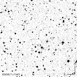
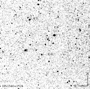
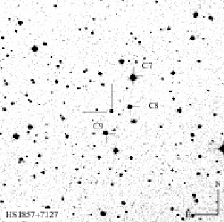
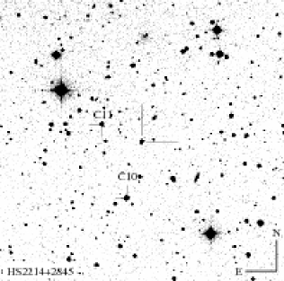
Figure 1: $10\arcmin\times 10\arcmin$ finding charts for HS 0417, HS 1016, HS 1340, HS 1857, and HS 2214 obtained from the Digitized Sky Survey. HS 2214 is the northern component of a close visual binary. See Table 3 for details on the comparison stars C1–C11.

1 Introduction

Dwarf novae are a subset of non- (or weakly) magnetic cataclysmic variables (CVs) that quasi-periodically brighten by several magnitudes. The commonly accepted cause for dwarf nova outbursts is a thermal instability in the accretion disc (e.g. Cannizzo et al., 1986; Osaki, 1996). Within this theoretical framework, accretion discs undergo outbursts if the accretion rate is below a critical value, $\dot{M}_{\mathrm{crit}}$. Above the $2-3$ h period gap, the mass transfer rate in CVs is typically larger than $\dot{M}_{\mathrm{crit}}$, and consequently only $\sim 36$ % of non-magnetic CVs with $\mbox{$P_{\rm orb}$}>3$ h are dwarf novae. For $\mbox{$P_{\rm orb}$}<3$ h, the fraction of confirmed dwarf novae among the short-period non-magnetic CVs is $\sim 83$ %. The large difference in mass transfer rate between short and long period systems is explained within the standard CV evolution theory by the cessation of magnetic braking – the dominant angular momentum loss mechanism in long period CVs –  once the systems evolve down to 3 h. Below $\mbox{$P_{\rm orb}$}=3$ h, the evolution of CVs proceeds much slower due to lower mass transfer rates driven by gravitational radiation as the angular momentum loss mechanism (e.g. Rappaport et al., 1983; Spruit & Ritter, 1983; King, 1988). For such low mass transfer rates, the disc instability model predicts thermally unstable accretion discs that produce dwarf-nova outbursts(Cannizzo, 1993; Osaki, 1996). Because of the long evolution time scale of low-mass transfer CVs population models built upon the disrupted magnetic braking scenario predict that 99% of all CVs should have periods below $3$ h (Kolb, 1993; Howell et al., 1997), which implies that the vast majority of all CVs is expected to be dwarf novae. Based on the current numbers, it appears that we know only a relatively small fraction of the predicted short-period CV population. Another prediction made by the population models is an accumulation of CVs near the minimum orbital period (e.g. Kolb & Baraffe, 1999), which is not observed. While this may signal a failure of the standard CV evolution theory (e.g. King et al., 2002; Barker & Kolb, 2003; Andronov et al., 2003), it is likely that the known sample of CVs is incomplete and biased. Dwarf novae are predominantly discovered because of their outbursts (Gänsicke, 2005), and hence CVs with very long outburst recurrence times or low-amplitude outbursts could be substantially underrepresented in the known CV population.

As a measure to probe the completeness of the known CV sample, we have initiated a search based on one property common to the majority of all CVs: the presence of Balmer emission lines in their optical spectra. We are selecting CV candidates from the Hamburg Quasar Survey (HQS, Hagen et al. 1995), an objective prism Schmidt survey of the northern hemisphere covering $13\,600\deg^{2}$ at high galactic latitudes with a limiting magnitude $17.5\la B\la 18.5$. The survey resulted in $\simeq 50$ new CVs, including a number of peculiar objects (e.g. Gänsicke et al., 2000; Rodríguez-Gil et al., 2004b, 2005b; Araujo-Betancor et al., 2005a); a general overview has been given by Gänsicke et al. (2002) and more recently by Aungwerojwit et al. (2005).

In this paper, we report the identification of five new dwarf novae in the HQS: HS 0417+7445, HS 1016+3412, HS 1340+1524, HS 1857+7127, and HS 2214+2845 (HS 0417, HS 1016, HS 1340, HS 1857, and HS 2214, respectively, hereafter; Fig. 1 and Table 1). In Sect. 2 we provide details about the observations and data reduction, in Sect. 3–7 we describe the data analysis and determine the orbital periods of the new dwarf novae. In Sect. 8, we compare the period distribution of the dwarf novae found in the HQS to that of all known dwarf novae. In Sect. 9 we discuss the implications of our survey work on the space density of CVs.

Table 1: Properties of the five new dwarf novae.

	HS 0417+7445	HS 1016+3412	HS 1340+1524	HS 1857+7127	HS 2214+2845
Right ascension (J2000)	$04^{\mathrm{h}}23^{\mathrm{m}}32.8^{\mathrm{s}}$	$10^{\mathrm{h}}19^{\mathrm{m}}47.3^{\mathrm{s}}$	$13^{\mathrm{h}}43^{\mathrm{m}}23.2^{\mathrm{s}}$	$18^{\mathrm{h}}57^{\mathrm{m}}20.4^{\mathrm{s}}$	$22^{\mathrm{h}}16^{\mathrm{m}}31.2^{\mathrm{s}}$
Declination (J2000)	$+74\degr 52\arcmin 50.30\arcsec$	$+33\degr 57\arcmin 53.9\arcsec$	$+15\degr 09\arcmin 16.9\arcsec$	$+71\degr 31\arcmin 19.2\arcsec$	$+29\degr 00\arcmin 20.6\arcsec$
Period (min)	$\simeq 105.1$/$\simeq 109.9$	$114.3\pm 2.7$	$92.66\pm 0.17$	$272.317\pm 0.001$	$258.02\pm 0.56$
Magnitude range	$18.0-13.5$	$18.6-15.4$:	$18.5-14.2$	$17.2-13.9$	$16.5-12.3$
${\mathrm{H}\alpha}$ EW [Å] / FHWM [Å]	172 / 43	184 / 27	121 / 28	39 / 32	53 / 33
${\mathrm{H}\beta}$ EW [Å] / FHWM [Å]	98 / 43	125 / 25	88 / 23	33 / 32	42 / 31
${\mathrm{H}\gamma}$ EW [Å] / FHWM [Å]	73 / 38	85 / 24	59 / 22	27 / 33	30 / 32
He I  $\lambda$5876 EW [Å] / FHWM [Å]	40 / 43	52 / 31	36 / 30	7 / 34	7 / 25
He I  $\lambda$6678 EW [Å] / FHWM [Å]	7 / 30	26 / 35	18 / 32	3 / 46	5 / 39
RASS source (1RXS J)	042332.8+745300	101946.7+335811	134323.1+150916	185722.6+713126	221631.2+290025
RASS count rate $\mathrm{(0.01\,cts\,s^{-1})}$	$6.0\pm 1.3$	$2.5\pm 1.0$	$7.3\pm 1.7$	$3.4\pm 4.5$	$9.9\pm 1.5$
Hardness ratio HR1	$1.00\pm 0.09$	$1.00\pm 0.91$	$0.18\pm 0.23$	$1.00\pm 0.04$	$0.92\pm 0.06$
Hardness ratio HR2	$0.21\pm 0.20$	$-0.32\pm 0.38$	$-0.05\pm 0.27$	$0.69\pm 0.10$	$0.10\pm 0.14$

Notes. The coordinates are taken from the USNO-B catalogue (Monet et al., 2003); the ROSAT PSPC count rates and hardness ratios HR1 and HR2 have been obtained from the ROSAT All Sky Survey (RASS) Bright Source Catalogue (Voges et al., 1999) and from the RASS Faint Source Catalogue (Voges et al., 2000); the ${\mathrm{H}\alpha}$–${\mathrm{H}\gamma}$ and He I  $\lambda$5876, 6678 equivalent widths (EW) and full width at half maximum (FWHM) were measured from the Calar Alto average spectra (Fig. 2) using the integrate/line task in MIDAS; the outburst of HS 1016 is uncertain (marked by a colon), as only one outburst was observed.

2 Observations and Data Reduction

2.1 Spectroscopy

Identification spectra of HS 0417, HS 1016, HS 1340, HS 1857, and HS 2214 were obtained at Calar Alto Observatory (Table 2). The spectra of all five systems (Fig.  2) contain strong Balmer emission lines on a blue continuum, together with weaker lines of He I that are characteristic of CVs. He II  $\lambda$4686 is very weak in all five systems, suggesting that they are dwarf novae observed in quiescence.

Additional time-resolved spectroscopy of HS 1016 (70 spectra), HS 1340 (78 spectra), HS 1857 (41 spectra), and HS 2214 (41 spectra) was obtained at the Calar Alto Observatory and Roque de los Muchachos Observatory (Table 2). The details of instrument setup and data reduction are described below.

Calar Alto Observatory.

Identification spectroscopy and time-resolved spectroscopy were obtained with the Calar Alto Faint Object Spectrograph (CAFOS) at the 2.2 m telescope throughout the period October 1996 to February 2005 (Table 2), with the exception of HS 1857 which was identified as a CV in 1990 using the B&C spectrograph on the 2.2 m telescope. The identification spectra were obtained either with the B-400 or the B-200 grating through a 1.5 ″slit on a $2\mathrm{k}\times 2\mathrm{k}$ pixel SITe CCD and were reduced with the MIDAS quicklook context available at the Calar Alto.

The time-resolved follow-up observations of HS 1016, HS 1340, HS 1857, and HS 2214 were obtained with the G-100 grating and a 1.2 ″slit, providing a spectral resolution of $\sim 4.1$ Å (full width at half maximum, FWHM) over the wavelength range $\lambda\lambda 4240-8300$. Clouds and/or moderate to poor seeing affected a substantial fraction of these observations. HS 2214 was observed under photometric conditions using the B-100 grating along with a 1.5″slit, providing a resolution of $\sim 4$ Å (FWHM) over the range 3500–6300 Å. Two additional red spectra of HS 2214 were taken with the R-100 grating, covering the range 6000–9200 Å at a similar resolution. All follow-up spectroscopy was obtained in 600 s exposures, interleaved with arc calibrations every $\sim 40$ min to correct for instrument flexure. Flux standards were observed at the beginning and end of the night – weather permitting –  to correct for the instrumental response. The data reduction (bias and flat-field correction, extraction, wavelength and flux calibration) was carried out using the Figaro package within Starlink and the programs Pamela and Molly developed by T. Marsh. Special care was given to the wavelength calibration by interpolating the dispersion relation for a given target spectrum from the two adjacent arc exposures.

Observatorio del Roque de los Muchachos.

The Intermediate Dispersion Spectrograph (IDS) together with a $2\mathrm{k}\times 4\mathrm{k}$ pixel EEV10a detector was mounted at the 2.5 m Isaac Newton Telescope (INT) on La Palma to obtain time-resolved spectroscopy of HS 1016, HS 1340, HS 1857, and HS 2214 (Table 2). The R632V grating and a slit width of 1.5 ″provided a spectral resolution of $\sim 2.3$ Å (FWHM) and a useful wavelength range of $\sim 4400-6800$ Å. The data reduction was carried out along the same lines as described above for the Calar Alto data using IRAF and Molly.

Table 2: Log of the observations.

Date	UT	Telescope	Filter/	Exp.	Frames	Comp.
			Grism	(s)		star
HS 0417+7445
1996 Oct 05	02:52	CA22	B-400	600	1	-
2000 Dec 21	22:41-02:37	WD	$B$	240	53	C1
2001 Jan 14	00:40-04:40	WD	$B$	240	54	C1
2003 Feb 27	20:35-23:47	OLT	$R$	300	37	C2
2004 Nov 12	17:40-02:03	WS	clear	150	162	C2
2005 Jan 03	02:18-04:40	INT	$g^{\prime}$	80	71	C2
2005 Jan 04	23:07-02:27	INT	$g^{\prime}$	30-35	162	C2
HS 1016+3412
2001 Apr 30	21:35	CA22	B-200	600	1	-
2003 Apr 07	21:54	CA22	G-100	600	1	-
2003 Apr 08	21:09-22:19	CA22	G-100	600	7	-
2003 Apr 10	22:28	CA22	G-100	600	1	-
2003 Apr 12	22:28-00:10	CA22	G-100	600	9	-
2003 Apr 24	22:07-23:01	INT	R632V	600	6	-
2003 Apr 25	23:31-00:24	INT	R632V	600	6	-
2003 Apr 27	22:27-23:28	CA22	G-100	600	6	-
2003 Apr 28	22:31-23:24	INT	R632V	600	6	-
2003 May 18	22:08-22:51	INT	R632V	600	6	-
2004 May 23	19:52-21:59	KY	clear	45-90	104	C3
2004 May 24	20:09-21:47	KY	clear	60	55	C3
2004 May 26	19:51-22:20	KY	clear	45	157	C3
2004 May 27	19:58-23:10	KY	clear	60-75	116	C3
2004 May 28	20:12-22:48	KY	clear	60	101	C3
2004 May 29	22:52-23:57	IAC80	clear	125	29	C3
2004 May 30	22:55-23:58	IAC80	clear	120	28	C3
2004 May 31	21:18-22:48	IAC80	clear	113	45	C3
2005 Feb 12	23:34-05:24	CA22	G-100	600	24	C3
HS 1340+1524
2001 May 01	02:14	CA22	B-200	600	1	-
2001 May 08	20:17-02:00	AIP	$R$	120	200	C6
2001 May 09	20:51-00:23	AIP	$R$	120	83	C6
2002 Jul 02	18:57-22:42	KY	$R$	120	86	C4
2002 Jul 04	20:02-22:17	KY	$R$	120	58	C4
2003 Apr 07	22:37-23:29	CA22	G-100	600	5	-
2003 Apr 08	22:42-23:41	CA22	G-100	600	6	-
2003 Apr 09	23:48-00:10	CA22	G-100	600	3	-
2003 Apr 10	22:46-00:29	CA22	G-100	600	7	-
2003 Apr 11	00:39-04:52	CA22	$V$	30	179	C4
2003 Apr 11	21:45-01:35	CA22	G-100	600	11	-
2003 Apr 13	00:31-03:28	CA22	G-100	600	12	-
2003 Apr 24	00:26-01:19	INT	R632V	600	6	-
2003 Apr 25	00:34-01:26	INT	R632V	600	6	-
2003 Apr 28	22:54-00:32	CA22	G-100	600	7	-
2003 May 29	19:44-22:03	KY	$R$	90	69	C4
2003 May 30	19:17-01:12	KY	$R$	90	212	C4
2003 Jun 24	19:28-22:08	KY	$R$	90	101	C4
2003 Jun 28	19:21-22:10	KY	$R$	120	76	C4
2004 Mar 17	07:18-11:38	FLWO	clear	40	297	C5

Date	UT	Telescope	Filter/	Exp.	Frames	Comp.
			Grism	(s)		star
2004 Mar 18	07:23-12:00	FLWO	clear	40	273	C5
2004 May 19	23:14-03:01	IAC80	clear	60	193	C6
2004 May 20	22:43-00:58	IAC80	clear	90	78	C6
2004 May 22	21:39-00:34	KY	clear	30	262	C4
2004 Jun 10	20:01-21:54	KY	clear	30	176	C4
2005 Feb 18	01:13-05:10	CA22	G-100	600	15	-
2005 May 11	23:10-03:04	IAC80	clear	45-60	203	C6
2005 May 12	22:41-04:20	IAC80	clear	60	213	C6
2005 May 13	22:07-04:09	IAC80	clear	60	270	C6
HS 1857+7127
1990 Jul 31	02:32	CA22	120 Å/mm	3600	1	-
2002 Apr 03	23:30-03:29	AIP	$R$	120	118	C9
2002 Apr 22	19:52-02:38	AIP	$R$	120	185	C9
2002 Sep 16	18:16-23:44	KY	$R$	5	1700	C8
2002 Sep 17	18:31-21:50	KY	$R$	5-10	683	C8
2002 Oct 24	18:05-04:27	AIP	$R$	60	447	C9
2003 Apr 08	02:44-03:44	CA22	G-100	600	6	-
2003 Apr 09	02:10-04:47	CA22	G-100	600	10	-
2003 Apr 13	02:25-04:50	CA22	G-100	600	9	-
2003 Apr 22	19:45-03:04	AIP	$R$	60	386	C9
2003 Apr 25	04:01-05:03	INT	R632V	600	7	-
2003 Apr 27	05:32-05:43	INT	R632V	600	2	-
2003 Apr 29	04:18-04:30	CA22	G-100	600	2	-
2003 Apr 29	04:46-05:28	INT	R632V	600	5	-
2003 Jul 08	03:18-05:19	OGS	clear	20	279	C7
2003 Aug 17	22:42-23:08	KY	$V$	8	147	C8
2003 Aug 17	03:28	HST/STIS	G140L	800	1	-
2004 May 03	00:21-05:46	IAC80	clear	15	922	C7
2004 May 03	06:11-07:53	FLWO	clear	10	487	C7
2004 May 04	08:25-11:15	FLWO	clear	10	809	C7
HS 2214+2845
2000 Sep 20	21:26	CA22	B-200	600	1	-
2000 Sep 21	03:28-11:04	BS	$R$	100	245	:
2000 Sep 24	02:44-10:53	BS	$R$	100	254	:
2000 Sep 24	20:10-23:55	CA22	B-100	600	16	-
2000 Sep 24	20:23-20:54	CA22	R-100	600	2	-
2002 Aug 29	02:25-03:48	INT	R632V	600	9	-
2002 Sep 01	03:07-03:58	INT	R632V	600	6	-
2002 Sep 02	02:51-03:22	INT	R632V	600	4	-
2002 Sep 04	00:23-00:54	INT	R632V	600	4	-
2003 Jun 23	23:54-02:08	KY	$R$	90	85	C11
2003 Jun 25	00:06-02:11	KY	$R$	90	80	C11
2003 Jun 27	23:35-00:44	KY	$R$	30	113	C11
2003 Jun 28	22:49-00:35	KY	$R$	60	93	C11
2003 Jul 15	02:29-05:09	OGS	clear	15	442	C10
2003 Sep 20	21:31-02:30	IAC80	clear	10	871	C10
2003 Sep 21	19:53-02:52	IAC80	clear	10	1187	C10
2003 Sep 22	20:14-03:10	IAC80	clear	10	772	C10
2003 Sep 24	00:16-03:59	IAC80	clear	10	689	C10

Notes. CA22: 2.2 m telescope at Calar Alto Observatory, using CAFOS with a $2\mathrm{k}\times 2\mathrm{k}$ SITe pixel CCD; WS: 0.8 m telescope at Wendelstein Observatory, using the MONICA CCD camera (Roth, 1992); OLT: 1.2 m Oskar Lühning Teleskop at Hamburg Observatory, equipped with a $1\mathrm{k}\times 1\mathrm{k}$ pixel SITe CCD; INT: 2.5 m Isaac Newton Telescope on Observatorio del Roque de los Muchachos, equipped with the Wide Field Camera (WFC), an array of four EEV $2\mathrm{k}\times 4\mathrm{k}$ pixel CCDs; KY: 1.2 m telescope at Kryoneri Observatory, using a Photometrics SI-502 $516\times 516$ pixel CCD camera; IAC80: 0.82 m telescope at Observatorio del Teide, equipped with Thomson $1\mathrm{k}\times 1\mathrm{k}$ pixel CCD camera; OGS: 1 m Optical Ground Station at Observatorio del Teide, equipped with Thomson $1\mathrm{k}\times 1\mathrm{k}$ pixel CCD camera; AIP: 0.7 m telescope of the Astrophysikalisches Institut Potsdam, using with $1\mathrm{k}\times 1\mathrm{k}$ pixel SITe CCD; FLWO: 1.2 m telescope at Fred Lawrence Whipple Observatory, equipped with the 4-Shooter CCD camera, an array of four $2\mathrm{k}\times 2\mathrm{k}$ pixel, only a small part of the CCD#3 was read out; BS: 0.41 m at Braeside Observatory telescope, using a SITe $512\times 512$ pixel CCD camera; the comparison stars used in instrumental magnitude extractions from Braeside are unknown (marked by colons).

Figure 2: Main panel: flux-calibrated CAFOS spectra of HS 0417, HS 1016, HS 1340, HS 1857, and HS 2214. Fluxes are labelled alternatingly on the left and right side. HS 1340 was observed in quiescence and outburst, respectively. Right panel: close-up plots of the ${\mathrm{H}\alpha}$ and ${\mathrm{H}\beta}$ profiles.

2.2 Photometry

Throughout the period December 2000 to May 2005, we obtained time-series differential CCD photometry of the five new dwarf novae during a total of 54 nights using ten different telescopes. The individual objects were observed for $\sim 25$ h (HS 0417), $\sim 14$ h (HS 1016), $\sim 68$ h (HS 1340), $\sim 50$ h (HS 1857), and $\sim 48$ h (HS 2214). Sample light curves are shown in Figs.  6 to 7. The details of the observations and instruments used are given in Table 2. The data obtained at Wendelstein, Calar Alto, Kryoneri, INT, and OLT were reduced using the pipeline described by Gänsicke et al. (2004a), which uses the Sextractor (Bertin & Arnouts, 1996) to calculate aperture photometry for all objects in the field of view. The AIP data were reduced entirely within MIDAS. Bias and flat-field correction of the OGS, IAC80, and FLWO images as well as the extraction of Point Spread Function (PSF) magnitudes was done using IRAF. For the Braeside data, the reduction was performed in a standard way using a custom-made software suite. Finding charts of all five dwarf novae are shown in Fig. 1. The comparison stars used in the reduction of our differential CCD photometry are listed in the last column of Table 2 (see Fig. 1 for identifications), and their USNO $R$ and $B$ magnitudes are given in Table 3.

Additional images of HS 0417, HS 1016, HS 1340, and HS 2214 were taken intermittently during the period May 2004 to April 2005 using the 0.37 m robotic Rigel telescope of the University of Iowa which is equipped with a $1\mathrm{k}\times 1\mathrm{k}$ pixel SITe-003 CCD camera. For all four systems, filterless images with an exposure time of 25s were obtained.

Figure 3: Sample light curves of HS 0417 obtained at the Wendelstein observatory. Top panel: $B$-band data obtained during superoutburst on January 14, 2001. Bottom panel: filterless data obtained during quiescence.

Figure 4: Sample filterless light curves of HS 1016 obtained at the Kryoneri observatory.

Figure 5: Sample light curves of HS 1340. Top panel: $R$-band data obtained at the Kryoneri observatory. Bottom panel: filterless data obtained at the IAC80 telescope.

Figure 6: Sample $R$-band light curves of HS 2214 obtained at the Braeside observatory.

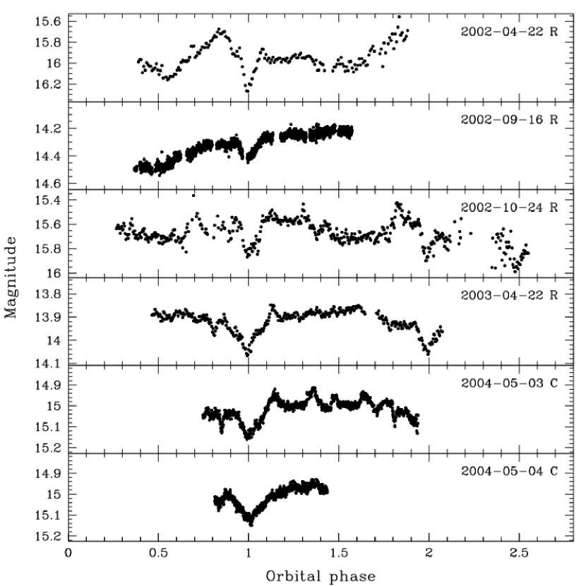
Figure 7: Sample $R$-band and filterless light curves of HS 1857 folded over the ephemeris in Eq. 1. See Sect. 6.2 for details.

2.3 The new dwarf novae as X-ray sources

All five dwarf novae identified on the basis of their emission line spectra in the HQS are also X-ray sources in the ROSAT All Sky Survey (RASS): HS 0417, HS 1340, and HS 2214 are contained in the Bright Source Catalogue (Voges et al., 1999), HS 1016 and HS 1857 within the Faint Source Catalogue (Voges et al., 2000). The X-ray properties of the new systems are summarised in Table 1. All but HS 1340 are hard X-ray sources in the hardness ratio HR1, typical of non- (or weakly-) magnetic CVs (van Teeseling et al., 1996).

Table 3: Comparison stars used for the differential CCD photometry of HS 0417, HS 1016, HS 1340, HS 1857, and HS 2214, see Fig. 1.

ID	USNO-A2.0	$R$	$B$
C1	1575-02009718	13.3	13.3
C2	1575-02008711	13.6	14.9
C3	1200-06495553	14.3	15.0
C4	1050-06991669	13.4	14.5
C5	1050-06992410	14.4	16.4
C6	1050-06992029	15.3	17.3
C7	1575-04072972	12.2	13.5
C8	1575-04073098	13.8	14.8
C9	1575-04073991	13.8	14.9
C10	1125-19198939	13.7	14.8
C11	1125-19199670	15.0	15.6

3 HS 0417+7445

Our identification spectrum of HS 0417 obtained in October 1996 (Fig. 2, Table 2) is dominated by low-excitation emission lines, typical of a dwarf nova. HS 0417 is contained in the ROSAT Bright Source Catalogue as 1RXS J042332+745300 (Voges et al., 1999), and has been independently identified as a CV by Wu et al. (2001). HS 0417 displayed large-amplitude variability on the HQS spectral plates, where it was detected at $B\simeq 18.0$ in June 1992 and at $B\simeq 13.7$ in October 1995, supporting the suggested dwarf nova nature of the object.

Throughout our photometric observations we have found the object near a mean magnitude of $\simeq 17.5$ (December 2000: $B\simeq 17.9$, February 2003: $R\simeq 17.3$, November 2004: filterless $\simeq 17.6$, January 2005: $g^{\prime}\simeq 17.5$), consistent with the USNO-A2.0 measurements, $R\simeq 17.2$ and $B\simeq 16.8$, except during January 2001, when the system was found in an outburst near $B\simeq 13.5$. In the quiescent state, the light curve of HS 0417 is characterised by a double-humped pattern with a period of $\sim 100$ min (Fig.6, bottom panel). The light curve obtained during the January 2001 outburst (Fig. 6, top panel) reveals superhumps that identify HS 0417 as a SU UMa-type dwarf nova and therefore this outburst as a superoutburst. An additional outburst of HS 0417 was caught on the rise in April 10, 2005 by one of us (PS), and $\sim 3$ h, $V$-band data obtained by David Boyd on the evening of April 11, 2005 showed the object already declining again at a rate of $\sim 0.85$ mag $\mathrm{d^{-1}}$ and no evidence of superhumps was found. By April 18, the system reached again its quiescent magnitude of $V\simeq 17.5$.

In order to measure the orbital period of the system, a Scargle (1982) periodogram was computed within the MIDAS/TSA context from all quiescent data except the February 2003 observations which were of too poor a quality. The periodogram (Fig. 8) contains a fairly broad sequence of aliases spaced by 1 $\mathrm{d^{-1}}$ with the strongest signal at $13.7$ $\mathrm{d^{-1}}$ and a nearly equally strong signal at $13.1$ $\mathrm{d^{-1}}$. The high-frequency range of the periodogram of HS 0417 is nicely reproduced by the window function (shifted to 13.7 $\mathrm{d^{-1}}$ in the top panel of Fig. 8), but excess power is present at frequencies below 10 $\mathrm{d^{-1}}$, most likely associated with the short length of the observing runs. Sine-fits to the data result in the periods corresponding to the two highest peaks in the periodogram, $P\simeq 105.1$ min and $P\simeq 109.9$ min, respectively. We interpreted these values as possible orbital periods of HS 0417.

The Scargle periodogram computed from the superoutburst data obtained on January 14, 2001 (Fig. 6, top panel) provides a broad signal with a peak at $\simeq 13.3$ $\mathrm{d^{-1}}$, or $P\simeq 108.3$ min. The light curve folded over this period shows, however, a significant offset between the two observed superhump maxima. A periodogram computed using Schwarzenberg-Czerny’s (1996) analysis-of-variance (AOV) method using orthogonal polynomial fits to the data (implemented as ORT/TSA in MIDAS) results in a much narrower peak compared to the Scargle analysis, centred at $12.95$ $\mathrm{d^{-1}}$ ($P\simeq 111.2$ min). This period provides a clean folded light curve. This improvement in the period analysis underlines the fact that AOV-type methods provide better sensitivity for strongly non-sinusoidal signals (such as superhumps) compared to Fourier-transform based methods.

The analysis of our photometric data left us with two candidate orbital periods, $\mbox{$P_{\rm orb}$}=105.1$ min or $\mbox{$P_{\rm orb}$}=109.9$ min, and two candidate superhump periods, $\mbox{$P_{\rm sh}$}=108.3$ min or $\mbox{$P_{\rm sh}$}=111.2$ min. Table 4 lists the fractional superhump excess, $\epsilon=(\mbox{$P_{\rm sh}$}-\mbox{$P_{\rm orb}$})/\mbox{$P_{\rm orb}$}$ calculated from all possible combinations of the candidate periods. We consider cases (2) and (3) as very unlikely, as no dwarf nova with $\epsilon>5\%$ is found below the period gap and no short-period dwarf nova with a negative superhump excess is known (e.g. Nogami et al., 2000; Patterson et al., 2003; Rodríguez-Gil et al., 2005a). In fact, most dwarf novae with $\mbox{$P_{\rm orb}$}\sim 100-115$ min have $\epsilon\sim 3-4\%$ (Patterson et al., 2005), which would make case (1) look most likely. However, based on our data, we prefer case (4) as $\mbox{$P_{\rm sh}$}=111.2$ min gave the cleanest folded superhump light curve. In this case, HS 0417 would have a rather low value of $\epsilon$, similar only to KV And ($\mbox{$P_{\rm orb}$}=105.49(30)$ min) which has $\epsilon=0.0145$ (Patterson et al., 2003). An unambiguous determination of both $P_{\rm orb}$ and $P_{\rm sh}$ would be important, as $\epsilon$ may be used to estimate the mass ratio of a CV (Patterson et al., 2005).

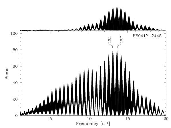
Figure 8: Main panel: the Scargle periodogram of HS 0417 during quiescence computed from all photometric data except February 27, 2003. Top panel: the window function shifted to 13.7 $\mathrm{d^{-1}}$.

Table 4: The fractional superhump excess of HS 0417 computed from $\epsilon=(\mbox{$P_{\rm sh}$}-\mbox{$P_{\rm orb}$})/\mbox{$P_{\rm orb}$}$.

Case	$P_{\rm orb}$ (min)	$P_{\rm sh}$ (min)	$\epsilon$
1	105.1	108.3	0.030
2	105.1	111.2	0.058
3	109.9	108.3	-0.015
4	109.9	111.2	0.012

4 HS 1016+3412

The CAFOS (Fig. 2) and INT average spectra of HS 1016 are similar to that of HS 0417, with strong Balmer emission lines together with weaker He I and Fe II lines and practically absent He II  $\lambda$4686. Our photometric time-series (Table 2) found the system consistently at a magnitude of $\simeq 17.5$. The system was found fainter, $V\simeq 18.6$, in the April 2003 CAFOS acquisition images. The only known outburst of HS 1016 was detected using the Rigel telescope on November 2, 2004, where an unfiltered magnitude of 15.4 was recorded. The next image obtained on November 11 showed the system again at its quiescent magnitude of $\simeq 17.5$.

The single-peaked profile found in the emission lines suggests a relatively low orbital inclination. No spectral contribution from the secondary star is detected in the red part of the spectrum. The equivalent widths (EWs) from the CAFOS and INT average spectra do not show any noticeable variation in each epoch throughout our run. Table 1 lists FWHM and EW parameters of the CAFOS average spectrum measured from Gaussian fits.

In order to determine the orbital period of HS 1016, we measured the radial velocity variation of ${\mathrm{H}\alpha}$, the strongest emission line, from the CAFOS and IDS spectra. We first rebinned the individual spectra to a uniform velocity centred on ${\mathrm{H}\alpha}$, followed by normalising the slope of the continuum. We then measured the ${\mathrm{H}\alpha}$ radial velocity variation using the double Gaussian method of Schneider & Young (1980) with a separation of 1000 $\mathrm{km\,s^{-1}}$ and an FWHM of 200 $\mathrm{km\,s^{-1}}$. A Scargle periodogram calculated from the ${\mathrm{H}\alpha}$ radial velocity variation contains a set of narrow aliases spaced by 1 $\mathrm{d^{-1}}$, with the strongest signal found at $f\simeq 12.6$ $\mathrm{d^{-1}}$ (Fig. 10, top panel). We tested the significance of this signal by creating a faked set of radial velocities computed from a sine function with a frequency of $12.6$ $\mathrm{d^{-1}}$, and randomly offset from the computed sine wave using the observed errors. The periodogram of the faked data set is plotted in a small window of the top panel in Fig. 10 which reproduces well the alias structure of the periodogram calculated from the observation. A sine-fit to the folded radial velocities refined the period to $114.3\pm 2.7$ min, which we interpreted as the orbital period of HS 1016. Figure 10 (top panel) shows a sine-fit to the phase-folded radial velocity curve; the fit parameters are reported in Table 5.

The light curves of HS 1016 display short-time scale flickering with an amplitude of $\sim 0.2-0.3$ mag (Fig. 6). A Scargle periodogram computed from the entire photometry as well as from individual subsets did not reveal any significant signal.

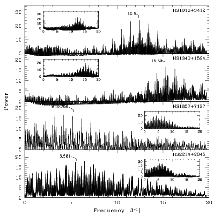
Figure 9: The Scargle periodogram of the radial velocities of HS 1016, HS 1340, HS 1857, and HS 2214. The periodograms constructed from faked sets of data at the corresponding orbital frequency are shown in small windows.

Figure 10: ${\mathrm{H}\alpha}$ radial velocities of HS 1016, HS 1340, and HS 1857 and ${\mathrm{H}\alpha}$ plus ${\mathrm{H}\beta}$ radial velocities of HS 2214. The radial velocities of HS 1016 and HS 1340 are folded on their spectroscopic periods of 114.3 min and 92.66 min, respectively and those of HS 1857 and HS 2214 folded on their photometric periods of 272.317 min and 258.02 min, respectively. The data on HS 1857 were folded using the eclipse ephemeris given in Eq. 1 while the other three systems were folded defining phase zero as the time of red-to-blue crossing of the radial velocities.

Table 5: Sine fits to the ${\mathrm{H}\alpha}$ radial velocities of HS 1016, HS,1340, and HS 1857. For HS 2214 a combination of ${\mathrm{H}\alpha}$ and ${\mathrm{H}\beta}$ radial velocities were fitted, as the September 2000 Calar Alto spectra did not cover ${\mathrm{H}\alpha}$. For HS 1857 and HS 2214, the periods were fixed to their values determined from the photometry.

Object	$T_{\mathrm{0}}$	Period (days)	K ($\mathrm{km\,s^{-1}}$)	$\gamma$ ($\mathrm{km\,s^{-1}}$)
HS 1016+3412	$2452737.4039\pm 0.0012$	$0.0794\pm 0.0019$	$93.0\pm 5.3$	$35.6\pm 3.9$
HS 1340+1524	$2452737.4438\pm 0.0018$	$0.06435\pm 0.00012$	$57.5\pm 6.2$	$-31.1\pm 4.1$
HS 1857+7127	$2452368.53243\pm 0.00098$	$0.189109\pm 0.000001$	$128.0\pm 9.6$	$-17.9\pm 7.4$
HS 2214+2845	$2451812.3309\pm 0.0028$	$0.17918\pm 0.00039$	$73.5\pm 6.5$	$29.8\pm 5.0$

5 HS 1340+1524

The average spectrum of HS 1340 during quiescence (Fig. 2) is similar to that of HS 0417 and HS 1016, showing strong single-peaked line profiles of Balmer emissions along with the weaker lines of He I and Fe II. The line parameters during quiescence are given in Table 1.

5.1 Long and short term variability

Throughout our time series photometry obtained at the AIP, IAC80, FLWO, and Kryoneri, HS 1340 was found at a mean magnitude in the range $\sim 17.7-16.8$ (see Fig. 11, main window). A first outburst of HS 1340 was detected on the evening of April 10, 2003 during observations with the 2.2m telescope at the Calar Alto Observatory (Table 2). The outburst peak magnitude was $V\simeq 14.7$ on the CAFOS acquisition image. The spectra obtained immediately thereafter show weak emission at ${\mathrm{H}\alpha}$, with an equivalent width of $\sim 4.7$ Å, whereas ${\mathrm{H}\beta}$ and ${\mathrm{H}\gamma}$ are in absorption with narrow emission cores, which are typical of an optically thick accretion disc. Similar spectra were observed in the three HQS CVs HS 0139+0559, HS 0229+8016, and HS 0642+5049 (Aungwerojwit et al., 2005). As the conditions during the night deteriorated, we switched to time-series photometry, recording a decline at $\sim 0.05\,\mathrm{mag\,hr^{-1}}$. The CAFOS acquisition images showed that HS 1340 faded to $V\simeq 16.1$ and $V\simeq 17.3$ in the two subsequent nights, April 11 and 12, 2003, respectively. A puzzling fact is that acquisition images taken before the outburst on April 7, 8, and 9, 2003 showed HS 1340 at $V\simeq 18.5$, i.e. nearly one magnitude fainter than the usual quiescent value (see Fig. 11, small window). On April 28, a CAFOS acquisition image showed the system again at a filterless magnitude of 17.6, consistent with the typical quiescent brightness. The duration of the entire outburst was less than two days.

A second outburst reaching an unfiltered magnitude of $\sim 14.2$ was recorded on April 15, 2005 with the Rigel telescope, again, the duration of the outburst was of the order of $2-3$ days.

The light curves of HS 1340 obtained during quiescence are predominantly characterised by variability on time scales of $\sim 15-20$ min with peak-to-peak amplitudes of $\sim 0.4$ mag (Fig.6, bottom panel). On some occasions, the light curves shows hump-like structures which last for one to several hours, superimposed by short-time scale flickering (e.g. Fig.6, top panel). Our period analysis of the photometric data did not reveal any stable signal in the combined data.

In summary, HS 1340 appears to have rather infrequent and short-lived outbursts, and displays a substantial amount of short-term variability as well as variability of its mean magnitude during quiescence.

5.2 The orbital period

The orbital period of HS 1340 was determined using the spectroscopic data taken in quiescence. The ${\mathrm{H}\alpha}$ radial velocity variation was measured in the same manner as in HS 1016 with a separation of 1000 $\mathrm{km\,s^{-1}}$ and an FWHM of 200 $\mathrm{km\,s^{-1}}$. Figure 10 (second panel) shows the Scargle periodogram. The strongest signal is found at $f=15.54\pm 0.03$ $\mathrm{d^{-1}}$ where the error is estimated from the FWHM of the strongest peak in the periodogram, corresponding to an orbital period of $\mbox{$P_{\rm orb}$}=92.66\pm 0.17$ min. The ${\mathrm{H}\alpha}$ radial velocity curve folded over this period is shown in Fig. 10 (second panel) along with a sine-fit; the fit parameters are given in Table  5. The periodogram of a faked data set constructed from this frequency agrees well with the entire observed alias structure (insert in Fig. 10, second panel).

With the spectroscopic period being determined, we re-analysed the time-series photometry of HS 1340, and found no significant signal in the range of the orbital frequency when we combined all quiescent data. However, a weak signal at a frequency of $\sim 15.5$ $\mathrm{d^{-1}}$ and its one-day aliases were detected intermittently on some occasions, e.g. in the 2003 Kryoneri data and the 2004 FLWO observations.

Figure 11: Main window: the mean magnitudes of HS1340 obtained from May 2001 to May 2005 in $R$-band (filled triangles), $V$-band (filled circles), and white light (open circles). The photometric error on the individual points is $<0.05$ mag. An additional systematic uncertainty arises from the combination of different band passes. Considering the apparent magnitudes of HS 1340 listed in the Sloan Digital Sky Survey which are $g=17.3$, $r=17.1$, and $i=17.1$, the errors due to colour terms are likely to be within $\pm 0.1$ mag. Small window: close up of the April 2003 CAFOS run. The first three points show the deep faint state with a mean magnitude of $V\simeq 18.5$ before the outburst on April 10, 2003.

6 HS 1857+7127

The CAFOS average spectrum of HS 1857 (Fig. 2) is similar to the spectra of HS 0417, HS 1016, and HS 1340, presenting a blue slope superimposed by Balmer and He I emission lines. Slight flux depressions are observed near 6200 Å and 7200 Å, which might be associated with the TiO bands of an M-type donor, however, the quality of the data is insufficient to unambiguously establish the detection of the secondary star. The Balmer emission line profiles are double-peaked, with a peak-to-peak separation of $\sim 800$ $\mathrm{km\,s^{-1}}$, suggesting a moderate to high inclination of the system. A high orbital inclination of HS 1857 was confirmed by the detection of eclipses in the light curves of the system (Fig. 7).

6.1 Long term variability

Throughout our photometric observing runs, HS 1857 was found to vary over a relatively large range between $17.2-13.9$ mag in average brightness, suggesting a frequent outburst activity (Fig. 7). Combined with the long orbital period (see below), it appears likely that HS 1857 is a Z Cam-type dwarf nova. The INT spectra obtained in April 2003 showed the system with a broad absorption trough around ${\mathrm{H}\beta}$, with a weak ($\mathrm{EW}\sim 3.5$ Å) single-peaked emission core, typical of dwarf novae during outburst (Hessman et al., 1984). As we did not obtain a spectrophotometric flux standard on that occasion, and have no simultaneous photometric data, the magnitude of that outburst could not be determined. An additional outburst spectrum was obtained in the ultraviolet using HST/STIS on August 17, 2003, showing a range of low and high ionisation lines of C, N, Si, and Al in absorption, as well as a P-Cygni profile in C IV  $\lambda$1550 (Fig. 12). We derived an $R$-band equivalent magnitude of 14.1 from the STIS acquisition image taken before the ultraviolet spectroscopy (see Araujo-Betancor et al. 2005b for details on the processing of STIS acquisition images), and ground-based photometry obtained at Kryoneri a few hours after the STIS observations found HS 1857 at $V=13.9$. The STIS spectrum resembles qualitatively the ultraviolet spectrum of Z Cam obtained during an outburst (Knigge et al., 1997). The P-Cygni profile provides evidence for the presence of a wind outflow during the outburst.

Figure 12: The HST/STIS spectrum of HS 1857 taken on August 17, 2003 during an outburst.

6.2 Eclipse ephemeris

We obtained light curves of HS 1857 throughout the period 2002 and 2004 and covered nine eclipses. We measured the times of the eclipse minima, and determined the cycle count by fitting $(\phi_{0}^{\mathrm{\mathrm{fit}}}-\phi_{0}^{\mathrm{observed}})^{-2}$ , leaving the period as a free parameter (Fig. 13). The following ephemeris was derived as:

$$\phi_{0}=\mathrm{HJD}\,2452368.53243(98)+0.189109(1)\times E$$ (1)

where $\phi_{0}$ is defined as the phase of mid-eclipse. The errors (given in brackets) of the zero phase and period were determined from a least-squares fit to the observed eclipse times versus the cycle count number. We conclude that the orbital period of HS 1857 is $\mbox{$P_{\rm orb}$}=272.317(1)$ min.

Table 6: The times of eclipse minima of HS 1857 obtained during the 2002 to 2004 runs .

Date	Eclipse minima (HJD)
2002 Apr 03	2452368.53446
2002 Apr 22	2452387.44260
2002 Sep 16	2452534.38100
2002 Oct 24	2452572.39500, 2452572.57893
2003 Apr 22	2452752.42275, 2452752.61229
2004 May 03	2453128.56222
2004 May 04	2453129.88816

The overall shape of the light curves and that of the eclipse profiles show a large degree of variability (Fig. 7). On April 22, 2002, the light curve shows an orbital modulation with a bright hump preceding the eclipse, typically observed in quiescent eclipsing dwarf novae (e.g. Zhang & Robinson, 1987), produced by the bright spot. A shallow ($\sim 0.4$ mag) eclipse is recorded, implying a partial eclipse of the accretion disc in the system. On September 16, 2002, the system was apparently caught on the rise to an outburst, with the eclipse depth reduced to $\sim 0.2$ mag. During several intermediate and bright states the signature of the bright spot disappeared, and was replaced by a broad orbital modulation with maximum light near phase 0.5, superimposed by short time scale flickering (Fig. 7, bottom four panels). On May 3, 2004, a narrow dip ($\Delta\phi\simeq 0.05$) centred at $\phi\simeq 0.8$ preceds the eclipse during both observed cycles. A similar feature, though of lower depth, has been observed on April 22, 2003.

6.3 Radial velocities

As for HS 1016 and HS 1340, we measured the ${\mathrm{H}\alpha}$ radial velocities of HS 1857 using the double-Gaussian method with a separation of 1500 $\mathrm{km\,s^{-1}}$ and an FWHM of 400 $\mathrm{km\,s^{-1}}$. The Scargle periodogram computed from these data contains a set of narrow peaks at 3.3 $\mathrm{d^{-1}}$, 4.3 $\mathrm{d^{-1}}$, and 5.3 $\mathrm{d^{-1}}$, consistent with the photometric frequency, $f\simeq 5.29$ $\mathrm{d^{-1}}$, computed from the eclipse ephemeris in the previous section, and its one-day aliases (Fig. 10, third panel). A periodogram calculated from a faked data set assuming the photometric frequency of $5.28796$ $\mathrm{d^{-1}}$, is shown in the insert in Fig. 10 (third panel). We folded the ${\mathrm{H}\alpha}$ radial velocity curve using the eclipse ephemeris given in Eq. 1, resulting in a quasi-sinusoidal modulation with an amplitude of $128.0\pm 9.6$ $\mathrm{km\,s^{-1}}$ and $\gamma=-17.9\pm 7.4$ $\mathrm{km\,s^{-1}}$, as determined from a sine-fit (Table 5). The red-to-blue crossing of the ${\mathrm{H}\alpha}$ radial velocities occurs at the photometric phase $\sim 0.1$ (Fig. 10, third panel). Such a shift is not too much of a surprise, as our radial velocity measurements were extracted from spectra sampling different brightness (outburst) states of HS 1857, covering less than one orbital cycle in all cases, and are not expected to represent a uniform and symmetrical emission from the accretion disc.

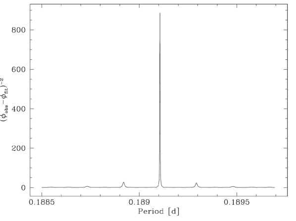
Figure 13: The periodogram of HS 1857 computed from nine eclipses obtained during the 2002 to 2004 runs.

7 HS 2214+2845

The CAFOS average spectrum of HS 2214 (Fig.  2) is characterised by a fairly red continuum superimposed by strong Balmer emission lines and weaker emission lines of He I, He II, and Fe II. The Balmer line profiles are double-peaked with a peak-to-peak separation of $\sim 800-1000$ $\mathrm{km\,s^{-1}}$, suggesting an origin in an accretion disc (Horne & Marsh, 1986). TiO absorption bands are present in the red part of the spectrum, revealing the late-type secondary star.

During our spectroscopic and photometric follow-up studies, HS 2214 was consistently found at $16.5-15.5$ mag, with night-to-night variations of the mean magnitude of $0.2-0.4$ mag. The dwarf nova nature of HS 2214 was confirmed through the visual monitoring by one of us (PS), which led to the detection of outbursts on December 10, 2004, and on May 2, July 14, September 22, 2005, and April 23, 2006. The mean cycle length appears to be $\sim 71$ d, and the maximum brightness recorded during outburst was $V\simeq 12.3$.

7.1 The spectral type of the secondary and distance

Overall, the spectrum of HS 2214 resembles that of the U Gem-type dwarf novae, e.g. CZ Ori (Ringwald et al., 1994), PG 0935+075 (Thorstensen & Taylor, 2001), and U Gem itself (Wade, 1979; Stauffer et al., 1979), which have secondary stars with spectral types in the range M2–M4, and orbital periods in the range 255–315 min.

In order to determine the spectral type of the secondary star in HS 2214, we used a library of spectral templates created from Sloan Digital Sky Survey data, covering spectral types M0–M9. For each spectral type, we varied the flux contribution of the M-dwarf template until the molecular absorption bands cancelled out as much as possible in the difference spectrum of HS 2214 minus template. The best match in the relative strength of the TiO absorption bands is achieved for a spectral type M$2.5\pm 0.5$, contributing 25% of the observed $V$-band flux of HS 2214 (Fig. 14). The extrapolated $JHK_{\mathrm{s}}$ spectrum of the secondary star agrees fairly well with the 2MASS $JHK_{\mathrm{s}}$ magnitudes of HS 2214 (14.5, 13.9, and 13.5, respectively), suggesting that the accretion disc contributes only a small amount to the infrared flux.

Using Beuermann & Weichhold’s (1999) calibration of the surface brightness in the 7165/7500 Å TiO band, and assuming a radius of $R_{2}=(3.0\pm 0.3)\times 10^{10}$ cm, based on the orbital period determined below and various radius-orbital period relations (e.g. Warner, 1995; Beuermann & Weichhold, 1999), we estimate the distance of HS 2214 to be $d=390\pm 40$ pc, where the error is dominated by the uncertainty of the secondary’s radius.

7.2 The orbital period

We first measured the radial velocity variation of ${\mathrm{H}\alpha}$ in the INT spectra and in the CAFOS spectra taken with the R-100 grism, as well as that of ${\mathrm{H}\beta}$ in the B-100 CAFOS spectra by using the double Gaussian method of Schneider & Young (1980). The Scargle periodogram calculated from these measurements contained a peak near $\sim 5.5$ $\mathrm{d^{-1}}$, but was overall of poor quality. In a second attempt, we determined the ${\mathrm{H}\alpha}$ and ${\mathrm{H}\beta}$ radial velocities by means of the $V/R$ ratios, calculated from having equal fluxes in the blue and red line wing, fixing the width of the line to $\sim 2500$ $\mathrm{km\,s^{-1}}$ in order to avoid contamination by the He I  $\lambda$6678 line adjacent to ${\mathrm{H}\alpha}$. The Scargle periodogram calculated from these sets of radial velocities contains the strongest signal at $6.6$ $\mathrm{d^{-1}}$ and an 1 $\mathrm{d^{-1}}$ alias of similar strength at $5.6$ $\mathrm{d^{-1}}$ (see Fig. 10, bottom panel). Based on the spectroscopy alone, an unambiguous period determination is not possible.

A crucial clue in determining the orbital period of HS 2214 came from the analysis of the two longest photometric time series obtained at the Braeside Observatory in September 2000 (Fig. 6). These light curves display a double-humped structure with a period of $\sim 4$ h, superimposed by relatively low-amplitude flickering. The analysis-of-variance periodogram (AOV, Schwarzenberg-Czerny, 1989) calculated from these two light curves contains two clusters of signals in the range of $4-7$ $\mathrm{d^{-1}}$and $10-13$ $\mathrm{d^{-1}}$, respectively (see Fig. 15). The strongest peaks in the first cluster are found at $\simeq 5.58$ $\mathrm{d^{-1}}$and $\simeq 5.92$ $\mathrm{d^{-1}}$  and at $\simeq 11.14$ $\mathrm{d^{-1}}$and $\simeq 11.48$ $\mathrm{d^{-1}}$ in the second cluster. Based on the fact that two of the frequencies are commensurate, we identify $f_{1}=5.58$ $\mathrm{d^{-1}}$ and $f_{2}=11.14$ $\mathrm{d^{-1}}$ as the correct frequencies, with $f_{1}$ being the fundamental and $f_{2}$ its harmonic. The periodogram of a faked data set computed from a sine wave with a frequency of $5.58$ $\mathrm{d^{-1}}$, evaluated at the times of the observations and offset by the randomised observational errors reproduces the alias structure observed in the periodogram of the data over the range $4-7$ $\mathrm{d^{-1}}$ very well (Fig. 15, top panel). A two-frequency sine fit with $f_{2}=2\times f_{1}$ to the data results in $f_{1}=5.581(12)$ $\mathrm{d^{-1}}$. The Braeside photometry folded over that frequency displays a double-hump structure (Fig. 16, two bottom panels). We identify $f_{1}$ as the orbital frequency of the system, hence, $\mbox{$P_{\rm orb}$}=258.02(56)$ min based on the following arguments. (a) The fundamental frequency detected in the photometry coincides with that of the second-strongest peak in the periodogram determined from the ${\mathrm{H}\alpha}$ and ${\mathrm{H}\beta}$ $V/R$-ratio radial velocity measurements (Fig.  10, bottom panel). (b) Double-humped orbital light curves are observed in a large number of short-period dwarf novae, e.g. WX Cet (Rogoziecki & Schwarzenberg-Czerny, 2001), WZ Sge (Patterson, 1998), RZ Leo, BC UMa, MM Hya, AO Oct, HV Vir (Patterson et al., 2003), HS 2331+3905 (Araujo-Betancor et al., 2005a), and HS 2219+1824 (Rodríguez-Gil et al., 2005a); the origin of those double-humps is not really understood, but most likely associated with the accretion disc/bright spot. In long-period dwarf novae, double-humped light curves are observed in the red part of the spectrum caused by ellipsoidal modulation of the secondary star, e.g. U Gem (Berriman et al., 1983) or IP Peg (Szkody & Mateo, 1986; Martin et al., 1987). In both cases, a strong and sometimes dominant, signal at the harmonic of the orbital period is seen in the periodogram calculated from their light curves.

Figure 10 (bottom panel) shows the radial velocity data folded over the photometric orbital period (258.02 min), along with a sine-fit (Table 5). The radial velocities are shown again in Fig. 16 together with the Braeside photometry, all folded using the photometric period but the spectroscopic zeropoint (Table 5). The photometric minima occur near orbital phase zero (inferior conjunction of the secondary) and 0.5, consistent with what is expected for ellipsoidal modulation. Very similar phasing is observed also for the double-humps in short-period systems, e.g. WZ Sge (Patterson, 1980) shows maximum brightness close to phases 0.25 and 0.75. However, given the strong contribution of the secondary star to optical flux of HS 2214 (Fig. 14), and the fact that the filterless Braeside photometry is rather sensitive in the red, we believe that the origin of the double-hump pattern seen in HS 2214 is indeed ellipsoidal modulation.

The binary parameters of HS 2214 could be improved in a future study by a measurement of the radial velocity of the secondary star, e.g. in using the Na doublet the $I$ band, and a determination of the orbital inclination from modelling the ellipsoidal modulation.

Figure 14: The average CAFOS spectrum of HS 2214 (black line) along with the best-matching M-dwarf template of spectral type M2.5, scaled to fit the strength of the molecular bands in HS 2214. The 2MASS $JHK_{\mathrm{s}}$ infrared fluxes of HS 2214 are represented by filled triangles, the $JHK$ spectrum of the M-dwarf template is shown as gray dots.

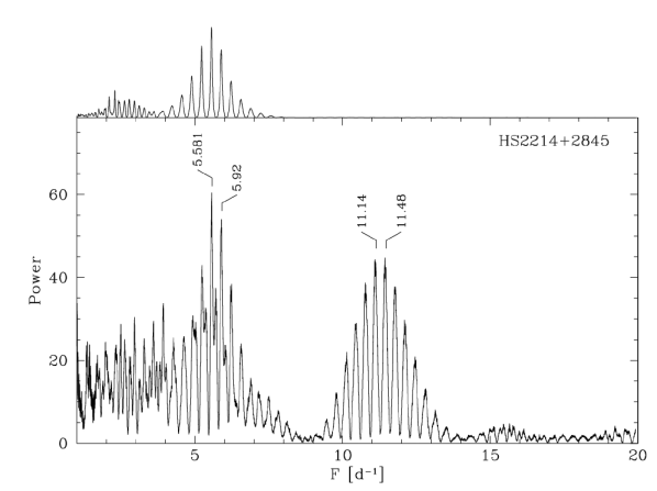
Figure 15: Main panel: the analysis-of-variance (AOV) periodogram of HS 2214+2845 calculated from the two longest light curves obtained at the Braeside Observatory, which show a double-humped pattern. Top panel: the AOV periodogram created from a sine wave with the orbital period of 258.02 min.

Figure 16: The spectroscopic and photometric data of HS 2214 are folded on the photometric period of 258.02 min using the spectroscopic zero-point $T_{0}=\mathrm{HJD}\,2451812.3309$ defined by the red-to-blue crossing of the ${\mathrm{H}\alpha}$ and ${\mathrm{H}\beta}$ radial velocities. In that phase convention, the inferior conjunction of the secondary star is expected at orbital phase zero. Top panel: the radial velocity variation of the ${\mathrm{H}\alpha}$ and ${\mathrm{H}\beta}$ emission lines, as already shown in Fig. 10. A whole cycle has been repeated for clarity. Middle panel: the photometric data obtained from the Braeside Observatory. Bottom panel: the photometric data binned into 25 phase slots, along with a two-frequency sine fit (dashed line).

8 The orbital period distribution of dwarf novae

Because of their outbursts, the vast majority of all currently known dwarf novae have been discovered by variability surveys, either through professional sky patrols, or through the concentrated efforts of a large number of amateur astronomers (Gänsicke, 2005). Considering the irregular temporal sampling of such observations, the population of known dwarf novae is likely to be biased towards systems which have frequent and/or large amplitude outbursts.

Figure 17: Top panel: the orbital period distribution of known CVs and dwarf novae from Ritter & Kolb (2003, 7th Edition, rev. 7.5, July 2005) are shown in gray and shade, respectively. Bottom panel: the period distribution of known dwarf novae according to their subtype, U Gem (UG), Z Cam (ZC), SU UMa (SU), WZ Sge (WZ), ER UMa (ER), and unclassified subtype (XX). The dashed lines are the conventional 2–3 h period gap.

Figure 18: Top panel: the orbital period distribution of 41 new CVs and 14 dwarf novae identified in HQS are shown in gray and shade, respectively. Bottom panel: the period distribution of HQS dwarf novae according to their subtype, U Gem (UG), Z Cam (ZC), SU UMa (SU), WZ Sge (WZ), and unclassified subtype (XX). The dashed lines are the conventional 2–3 h period gap.

Table 7: Dwarf novae discovered in the HQS with their subtype, U Gem (UG), SU UMa (SU), Z Cam (ZC), and unclassified (XX). Uncertain classifications are marked by a colon.

HQS ID	Other name	$P_{\rm orb}$ (min)	Type	References
HS 2331+3905		81.1	WZ:	1
HS 1449+6415	KV Dra	84.9	SU	2,3
HS 2219+1824		86.3	SU	4
HS 1340+1524		92.7	XX	5
HS 1017+5319	KS UMa	97.9	SU	2,6
HS 0417+7445		105.1/109.9	SU	5
HS 1016+3412		114.3	XX	5
HS 0913+0913	GZ Cnc	127.1	XX	2,8,9
HS 0941+0411	RX J0944.5+0357	215.0	XX	2,10
HS 0552+6753	LU Cam	216.6	UG	2,7
HS 0907+1902	GY Cnc	252.6	UG	2,11
HS 2214+2845		258.0	UG	5
HS 1857+7127		272.3	ZC:	5
HS 1804+6753	EX Dra	302.3	UG	12,13,14

References: (1) Araujo-Betancor et al. (2005a); (2) Jiang et al. (2000); (3) Nogami et al. (2000); (4) Rodríguez-Gil et al. (2005a); (5) this work; (6) Patterson et al. (2003); (7) Thorstensen priv. com. & vsnet-campaign-dn 2681; (8) Kato et al. (2002); (9) Tappert & Bianchini (2003); (10) Mennickent et al. (2002); (11) Gänsicke et al. (2000); (12) Fiedler et al. (1997); (13) Billington et al. (1996); (14) Shafter & Holland (2003).

8.1 The orbital period distribution of all known dwarf novae

Inspecting the Ritter & Kolb catalogue (2003, Edition 7.5 of July 1, 2005) within the orbital period range of $\sim 1$ h to $\sim 1$ d and removing AM CVn systems, it is found that nearly half of all known CVs (262 systems out of 572, or 46%) are dwarf novae of which 166 (63%) have $\mbox{$P_{\rm orb}$}<2$ h, 26 (10%) are found in the $2-3$ h orbital period gap, and 70 (27%) have long periods, $\mbox{$P_{\rm orb}$}>3$ h. The conventional definition of the period gap as being the range $2-3$ h is somewhat arbitrary, and these numbers vary slightly if a different definition is used, but without changing the overall picture. Figure 18 (top panel) shows the orbital period distribution of all known CVs and dwarf novae with periods between $\sim 1$ h and $\sim 1$ d. Whereas the total population of all CVs features the well-known period gap, i.e. the relatively small number of CVs with periods $2$ h$\,<\mbox{$P_{\rm orb}$}<3$ h, the number of dwarf nova reaches a minimum in the range $3-4$ h. In fact, the number of dwarf nova with $3$ h$\,<\mbox{$P_{\rm orb}$}<4$ h is a half (15, or 6% of all dwarf novae) of that in the “standard” $2-3$ h period gap (26, or 10%). The dearth of known dwarf novae in the $3-4$ h period range was pointed out by Shafter et al. (1986) and Shafter (1992), who compared the observed dwarf nova period distribution with those constructed from various magnetic braking models, and concluded that none of the standard magnetic braking models can satisfactorily explain the lack of observed dwarf novae in the $3-4$ h period range.

The bottom panel of Fig. 18 displays all known dwarf novae according to their subtypes which are 159 (61%) SU UMa, 37 (14%) U Gem, 18 (7%) Z Cam, and 48 (18%) unclassified subtypes (XX). For completeness, we note that the SU UMa class includes 8 ER UMa stars (which have very short superoutburst cycles) and 19 WZ Sge stars (which have extremely long outburst cycles). All confirmed U Gem and Z Cam stars lie above the period gap, in fact all but one Z Cam star (BX Pup) have $\mbox{$P_{\rm orb}$}>3.5$ h. It is clearly seen that the majority (85%) of SU UMa lie below the period gap and only a small fraction (15%) inhabits the $2-3$ h period range.

The orbital period distribution of short-period dwarf novae in Fig. 18 (the majority of all CVs in this period range) differs markedly from the predictions made by the standard CV evolution theory (e.g. Kolb, 1993; Howell et al., 2001; Kolb & Baraffe, 1999): the minimum period is close to $\sim 77$ min, contrasting with the predicted minimum period of $\sim 65$ min (Paczyński & Sienkiewicz, 1983), and the distribution of systems is nearly flat in $P_{\rm orb}$, whereas the theory predicts a substantial accumulation of systems at the minimum period. Several modifications of the CV evolution theory have been suggested to resolve this discrepancy, however, none with undisputable success (King et al., 2002; Renvoizé et al., 2002; Barker & Kolb, 2003).

8.2 The orbital period distribution of dwarf novae in the HQS

Another possible explanation for the lack of a spike in the orbital period distribution of CVs near the minimum period is that systems close to the minimum period, especially those evolving back to longer periods, have not yet been discovered due to observational selection effects. As most CVs below the period gap are dwarf novae, the most obvious bias suppressing the period spike is to assume that dwarf novae close to the minimum period have very rare outbursts. In fact, a number of dwarf novae near the minimum period have very long outburst intervals, e.g. WZ Sge ($\mbox{$P_{\rm orb}$}=81.6$ min, Patterson et al. 2002) erupts every $20-30$ years; GW Lib ($\mbox{$P_{\rm orb}$}=76.8$ min, Thorstensen et al. 2002) has been seen in outburst only once in 1983. It can not be excluded that these systems represent “the tip of the iceberg” of a dwarf nova population with even longer outburst periods. Assuming that rarely outbursting dwarf novae do exist in a significant number, and that they spectroscopically resemble the known objects, such as WZ Sge or GW Lib, our search for CVs in the HQS should be able to identify them (Gänsicke et al., 2002).

We have so far obtained orbital periods for 41 new CVs found in the HQS, their period distribution is shown in Fig. 18 (top panel). The first thing to notice is that the majority of the new CVs identified in the HQS are found above the period gap, with a large number of systems in the period range $3-4$ h (for a discussion of the properties of CVs in this period range, see Aungwerojwit et al., 2005). As for the overall CV population, a dearth of systems is observed in the $2-3$ h period range (Fig. 18, top panel), with the gap being wider for dwarf novae (Fig. 18, bottom panel).

To date 14 (26%) out of 53 new CVs discovered in the HQS have been classified as dwarf novae, including the five systems, HS 0417, HS 1016, HS 1340, HS 1857, and HS 2214, presented in this paper (Table 7). The fraction of long-period ($\mbox{$P_{\rm orb}$}>3$ h) systems is larger in the HQS sample (43%) than in the total population of known dwarf novae (27%, see Sect. 8.1). The total number of new HQS dwarf novae is relatively small, and subject to corresponding statistical uncertainties. However, the tilt towards long-period dwarf novae among the new HQS CVs is likely to be underestimated, as a significant number of long-period HQS CVs have still uncertain CV subtypes, and several of them could turn out to be additional Z Cam-type dwarf nova (Aungwerojwit et al. 2005 plus additional unpublished data). Optical monitoring of the long-term variability of these systems will be necessary to unambiguously determine their CV type. Overall, the dwarf novae identified within the HQS fulfill the above expectations of being “low-activity” systems, i.e. dwarf novae that have either infrequent outbursts (e.g. KV Dra, HS 0941+0411, HS 2219+1824) or low-amplitude outbursts (e.g. EX Dra). We found only one system that resembles the WZ Sge stars with their very long outburst intervals found near the minimum period that is HS 2331+3905 (Araujo-Betancor et al., 2005a) which has a period of 81.1 min, and no outburst has been detected so far.

Thus, our search for CVs in the HQS has been unsuccessful in identifying the predicted large number of short-period CVs, despite having a very high efficiency in picking up systems that resemble the typical known short-period dwarf novae.

9 Constraints on the space density of CVs

CV population models result in space densities in the range $2\times 10^{-5}\,\mathrm{pc}^{-3}$ to $2\times 10^{-4}\,\mathrm{pc}^{-3}$ (de Kool, 1992; Politano, 1996), whereas the space density determined from observations is $(0.5-1)\times 10^{-5}\,\mathrm{pc}^{-3}$ (Patterson, 1984; Ringwald, 1996; Patterson, 1998). It appears therefore that we currently know about an order of magnitude less CVs than predicted by the models. Also the observed ratio of short to long orbital period systems is in strong disagreement with the predictions of the theory. Patterson (1984, 1998) estimated that the fraction of short-period CVs per volume is $75-80$%, which has to be compared to 99% in the population studies (Kolb, 1993; Howell et al., 1997).

Because of the large differences in mass transfer rates, and, hence, absolute magnitudes, of long ($\mbox{$P_{\rm orb}$}>3$ h) and short ($\mbox{$P_{\rm orb}$}<3$ h) period CVs, magnitude limited samples appear at a first glance utterly inappropriate for the discussion of CV space densities. However, taking the theoretical models at face value, the space density of long period CVs is entirely negligible compared to that of short period CVs (Kolb, 1993; Howell et al., 1997), and hence a discussion of the total CV space density can be carried out on the basis of short-period systems alone. In the following, we assess the expected numbers of systems in the HQS separately for short-period CVs that are still evolving towards the minimum period (pre-bounce), and those that already reached the minimum period, and evolve back to longer periods (post-bounce). For both cases, we assumed (1) a space density of $5\times 10^{-5}\,\mathrm{pc}^{-3}$ as an intermediate value between the predictions of de Kool (1992) and Politano (1996), (2) that 70% of all CVs are post-bounce systems, and 30% are pre-bounce systems (Kolb, 1993; Howell et al., 1997)(ignoring, as stated above, the small number of long-period CVs), (3) a scale height of 150 pc (e.g. Patterson, 1984), and (4) that the luminosity of short-period CVs is dominated by the accretion-heated white dwarf.

9.1 Pre-bounce CVs expected in the HQS

CV evolution models predict a typical accretion rate of $\dot{M}\simeq 5\times 10^{-11}\,\mbox{$\mathrm{\mbox{$M_{\odot}$}\,yr^{-1}}$}$ for pre-bounce systems, with a relatively small spread (Kolb, 1993; Howell et al., 1997). For this accretion rate, Townsley & Bildsten’s (2003) calculation of white dwarf accretion heating predicts an effective temperature of $T_{\mathrm{wd}}\simeq 12\,000$ K. If the luminosity is dominated by a white dwarf of this temperature, the HQS with an average magnitude limit of $B\simeq 18$ would detect pre-bounce CVs out to a distance of 175 pc (using the absolute magnitudes of white dwarfs by Bergeron et al. 1995), i.e. over a bit more than one scale height. Within a sphere of radius 175 pc around the Earth, one would expect $\simeq 144$ CVs (taking into account the exponential drop-off of systems perpendicular to the plane), of which $\simeq 36$ would be within the sky area sampled by the HQS. This is a conservative lower limit, as any additional luminosity from the accretion disc and/or bright spot as well as a hotter white dwarf temperature would increase the volume sampled by the HQS, and therefore increase the number of pre-bounce CVs within the survey.

9.2 Post-bounce CVs expected in the HQS

Once past the minimum period, the accretion rate of CVs substantially drops as a function of time, and we assume here a value of $\dot{M}=10^{-11}\,\mbox{$\mathrm{\mbox{$M_{\odot}$}\,yr^{-1}}$}$, corresponding to an intermediate CV age of $\sim 5$ Gyr (Kolb & Baraffe, 1999), and a white dwarf temperature of $T_{\mathrm{wd}}\simeq 7000$ K (Townsley & Bildsten, 2003). This lower white dwarf temperature reduces the detection limit of the HQS to only $\simeq 65$ pc. The total number of post-bounce CVs within a sphere of radius 65 pc around the Earth is hence expected to be 40, of which 10 within the HQS area.

9.3 Short-period CVs in the HQS: most likely pre-bounce only

The immediate question is what type are the short-period HQS CVs: pre- or post-bounce? As mentioned in Sect. 8.2, only 12 short-period ($\mbox{$P_{\rm orb}$}<3$ h) systems have been found among the 41 new HQS CVs for which we have adequate follow-up data. The new short-period CVs comprise 8 dwarf novae (Table  7), two polars (Reimers et al., 1999; Jiang et al., 2000; Schwarz et al., 2001; Tovmassian et al., 2001; Thorstensen & Fenton, 2002; Gänsicke et al., 2004b), one intermediate polar (Rodríguez-Gil et al., 2004a; Patterson et al., 2004), and one system with uncertain classification (Gänsicke et al., 2004a). The white dwarf has been detected in the spectra of HS 2237+8154 (Gänsicke et al., 2004a), HS 2331+3905 (Araujo-Betancor et al., 2005a), HS 2219+1824 (Rodríguez-Gil et al., 2005a), and HS 1552+2730 (Gänsicke et al., 2004b), with temperatures of $\simeq 10\,500$ K, $\simeq 11\,500$ K, $\simeq 15\,000$ K, and $\simeq 20\,000$ K, respectively. These four systems are very likely to have the lowest mass transfer rates among the 12 new short-period CVs, the optical spectra of the other eight are characterised by strong Balmer and He emission lines and the associated continuum which outshines the white dwarf, typical of higher accretion rates. While there are still about a dozen HQS CVs with no accurate orbital period determination, the data already at hand makes it very unlikely that more than 2 or 3 of those systems will turn out to have periods $<3$ h.

For a complete assessment of the short-period content of the HQS, one has obviously to include in the statistics the short-period CVs that are contained within the HQS data base, but were already known – subject to the same selection criteria that were applied to identify the twelve new systems. Gänsicke et al. (2002) analysed the properties of the previously known CVs within the HQS data base, and came to the following conclusions. 18 previously known short-period ($\mbox{$P_{\rm orb}$}<3$ h) systems with HQS spectra are correctly (re-)identified as CVs, including 12 dwarf novae, five polars, and one intermediate polar. Gänsicke et al. (2002) also found that only two previously known short-period systems with HQS spectra failed to be identified as CVs; this “hit rate” of 90% underlines the extreme efficiency of the HQS of finding short period CVs. Five out of those 18 systems have measured white dwarf temperatures, all of them in the range $\simeq 11\,000-16\,000$ K (MR Ser, ST LMi, AR UMa, SW UMa, T Leo: Gänsicke et al. 2001; Hamilton & Sion 2004; Araujo-Betancor et al. 2005b; Gänsicke et al. 2005). The remaining 13 systems all have spectra dominated by strong Balmer and He emission, suggesting accretion rates too high to detect the white dwarf.

In summary, the HQS contains a total of 30 short-period CVs (12 new identifications plus 18 previously known systems), all of which are consistent with being pre-bounce systems. At face value, this number agrees rather nicely with the 36 expected systems derived above, but one has to bear in mind that that number is an absolute lower limit, as hotter white dwarfs and/or accretion luminosity from the disc and hot spot will increase the volume sampled by the HQS.

While there may still be some shortfall of pre-bounce systems, it is much more worrying that so far no systems with the clear signature of a post-bounce CV that evolved significantly back to longer periods has been found – neither in the HQS, nor elsewhere. The coldest CV white dwarfs have been found, to our knowledge, in the polar EF Eri ($T_{\mathrm{wd}}\simeq 9500$ K, Beuermann et al. 2000), and HS 2331+3905 ($T_{\mathrm{wd}}\simeq 10\,500$ K, Araujo-Betancor et al. 2005a), both systems with orbital periods of $\simeq 81$ min – which may hence be either pre- or post-bounce systems.

A final note concerns the number of WZ Sge stars, i.e. short-period dwarf novae with extremely long outburst intervals. Given the strong Balmer lines in the known WZ Sge stars e.g. WZ Sge itself (Gilliland et al., 1986), BW Scl (Abbott et al., 1997), GD 552 (Hessman & Hopp, 1990), and GW Lib (Szkody et al., 2000; Thorstensen et al., 2002), we believe that any WZ Sge brighter than $B\simeq 18$ would have easily been identified in the HQS – yet, only a single new WZ Sge system has been discovered, HS 2331+3905 (Araujo-Betancor et al., 2005a).

Thus, we conclude that while our systematic effort in identifying new CVs leads to a space density of pre-bounce short period CVs which agrees with the predictions within an order of magnitude, the bulk of all CVs, which are predicted to have made it past the minimum orbital period, remains unidentified so far.

10 Conclusions

We have identified five new dwarf novae as part of our search for new CVs in the HQS, bringing the total number of HQS-discovered dwarf novae to 14. The new systems span orbital periods from $\sim 1.5$ h to nearly 5 h, confirming the trend that dwarf novae spectroscopically selected in the HQS display a larger ratio of long-to-short orbital periods. Overall, dwarf novae represent only about one third of the HQS CVs which are studied sufficiently well, and it is by now clear that the properties of the sample of new HQS CVs do not agree with those of the predicted large population of short-period low-mass-transfer systems. Within the limiting magnitude of $B\simeq 17.5-18.5$, the HQS does however contain a large number of previously known dwarf novae that were identified because of their variability, and almost all of these systems have been recovered as strong CV candidates on the basis of their HQS spectrum (Gänsicke et al., 2002). Based on their spectroscopic and photometric properties it appears that most, if not all short-period CVs in the HQS (newly identified and previously known) are still evolving towards the minimum period. If the large number of post-bounce CVs evolving back to longer periods predicted by population models exists, they must (a) have very long outburst recurrence times, and (b) have H$\beta$ equivalent widths that are far lower than observed in the currently known typical short-period CVs.