Low-mass star formation in R Coronae Australis: Observations of organic molecules with the APEX telescope

This paper presents new APEX submillimetre molecular line observations of three low-mass protostars, IRS7A, IRS7B, and IRAS32, in the R Coronae Australis molecular cloud complex. The molecular excitation analysis is performed using a statistical equilibrium radiative transfer code. The derived beam averaged fractional abundances vary by less than a factor of two among the three sources, except those of H₂CO and CH₃OH, which show differences of about an order of magnitude. The molecular abundances are similar to those typically found in other star-forming regions in the Galaxy, such as the $\rho$ Oph and Perseus molecular clouds. There is a marked difference in the kinetic temperatures derived for the protobinary source IRS7 from H₂CO ($\approx$ 40–60 K) and CH₃OH ($\approx$ 20 K), possibly indicating a difference in origin of the emission from these two molecules.

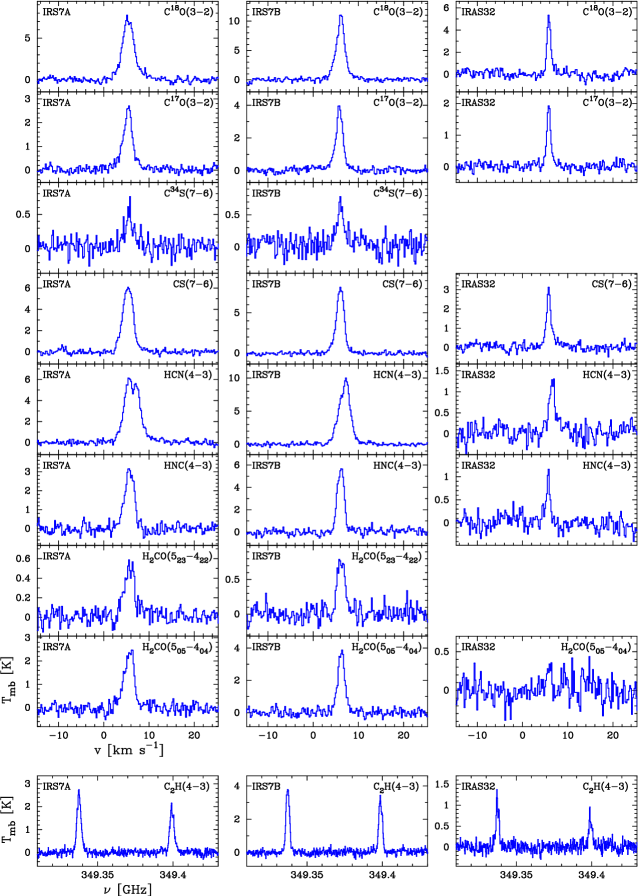
Figure 1: New observations of molecular line emission using the APEX telescope. The velocity resolution is 0.2 km s^-1 in all the spectra.

1 Introduction

In the earliest, deeply-embedded stage, low-mass protostars are surrounded by a collapsing envelope and a circumstellar disk. In this phase, the initial chemical composition of the disk is determined. The chemistry of molecules in the circumstellar envelope is likely to be directly reflected in the molecular composition in the disk, which forms the building blocks from which planets may form. An interesting aspect is the search for low-mass ’hot cores‘, i.e., regions where grain ice mantles are liberated in the envelope close to the central protostar because of its heating (e.g., Ceccarelli et al. 2000; Schöier et al. 2002; Cazaux et al. 2003). The search for hot cores around low-mass stars is not yet conclusive, mainly due to limitations in the available observational data. Also, outflows are likely to play an important role by affecting many of the same species thought to be sign posts of hot cores (e.g., Jørgensen et al. 2005). Moreover, the chemistry of traditional hot-core tracers such as H₂CO may be affected by the freeze-out of CO (e.g., Schöier et al. 2004), which is why combined studies of chemically related molecular species are important.

The R Coronae Australis dark cloud is a nearby (170 pc, Knude & Høg 1998) region of active star formation (e.g., Brown 1987; Chini et al. 2003; Nutter et al. 2005). Molecular line observations of protostellar objects in R Coronae Australis have attained little attention, mainly due to its location on the southern hemisphere. Previous studies using single-dish telescopes with limited spatial resolution, which are mainly sensitive to the chemistry of the outer cold regions of the envelopes, have been biased towards lower excitation lines. A wealth of molecular rotational transitions lying in the 279 $-$ 381 GHz window are accessible with APEX, and can be used to constrain the physics, and in particular, the chemistry in the dense ($>$ 10⁶ cm³) and warm ($>$ 30 K) material in the envelopes. Observations of protostellar objects in Corona Australis are also interesting for testing the importance of the surroundings on the formation of protostars, and will complement previous extensive studies in Perseus and $\rho$ Oph (Jørgensen et al. 2002, 2004, 2005). It is not clear how the properties of the parental cloud affect the properties of the emerging protostar (see Jayawardhana et al. 2001). Likewise, the properties of the parental cloud may reflect the chemical evolution of the protostar, for example, in the degree of freeze-out and the ’initial abundances‘.

The first step in a project aimed at obtaining an extensive data base of molecular line emission towards a large sample of protostars in the southern hemisphere, with a focus on the Corona Australis and Chameleon molecular clouds, is presented in this Letter. It is crucial to utilize APEX to build comparable samples of well-studied low-mass protostars for future ALMA observations

2 Observations

Observations of sub-millimetre molecular line emission towards the R Coronae Australis molecular cloud complex were performed September 4–6, 2005, using the 12 m APEX telescope equipped with an SIS receiver (APEX–2a). Typical system temperatures were in the range 140 $-$ 380 K (DSB). The 1 GHz FFTS with 8192 spectral channels was used as a backend, providing a spectral resolution of 122 kHz (0.1 km s^-1). The observations were carried out using a position-switching mode, with the reference position located at +2$\arcmin$ in azimuth. The data were reduced in a standard way by removing, in most cases, a low order ($\leq$ 3) polynomial baseline and the raw spectra, stored in the $T_{\mathrm{A}}^{\ast}$ scale, converted to main-beam brightness temperature using $T_{\mathrm{mb}}$ = $T_{\mathrm{A}}^{\ast}/\eta_{\mathrm{mb}}$. $T_{\mathrm{A}}^{\ast}$ is the antenna temperature corrected for atmospheric attenuation using the chopper-wheel method, and $\eta_{\mathrm{mb}}$ is the main-beam efficiency. A value of $\eta_{\mathrm{mb}}$ $=$ 0.7 was assumed for all spectral settings. Regular pointing checks were made on strong CO sources and typically found to be consistent within $\approx$ 3$\arcsec$. The FWHM of the main beam is 18″at 345 GHz. The uncertainty (including errors in pointing, calibration, and $\eta_{\mathrm{mb}}$) in the absolute intensity scale (main-beam brightness) is estimated to be about $\pm 15$%.

The observed spectra for the protostellar objects IRS7A ($\alpha_{2000}$ = 19:01:55.3, $\delta_{2000}$ = –36:57:21), IRS7B ($\alpha_{2000}$ = 19:01:56.4, $\delta_{2000}$ = –36:57:27), and IRAS32 ($\alpha_{2000}$ = 19:02:58.7, $\delta_{2000}$ = –37:07:34) are presented in Figs. 1 and 2 (the positions are obtained from IRAC4 8 $\mu$m pipeline data in the Spitzer Space Telescope archive: AOR ID 3650816). IRS7B is identified as a class 0 protostar, whereas IRS7A and IRAS32 are of class I (see Nutter et al. 2005, and references therein).

Results of Gaussian fits to the spectra are reported in Table 1. The systemic (LSR) velocities obtained from the Gaussian fits are 5.3, 5.6, and 5.9 km s^-1 (LSR) for IRS7A, IRS7B, and IRAS32, respectively. The spectra are generally well represented by a single Gaussian, with the major exception being the observed HCN $J$ = 4 $\rightarrow$ 3 line emission towards IRS7A and IRS7B. In these two cases, not only is the HCN line significantly broader, compared to other molecular lines, but also a central absorption dip is present, at least in the IRS7A spectrum. The HCN spectra presented here are very similar to those of HCO⁺ $J$ = 4 $\rightarrow$ 3 obtained by Anderson et al. (1997a). They interpret the emission as arising in a large rotating (circumbinary) disk, and the self-absorption feature is caused by absorption in a dense and quiescent foreground of the cloud. In addition, for the two IRS7 sources, our observed C¹⁷O and, in particular, C¹⁸O, $J$ = 3 $\rightarrow$ 2 spectra have weak wings, possibly related to the known molecular outflow in this region, and are somewhat better reproduced by a sum of two Gaussians.

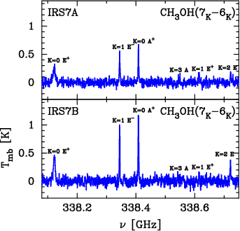
Figure 2: New observations of CH₃OH line emission using the APEX telescope. The velocity resolution is 0.5 km s^-1 in both spectra. Note that the $7_{0}$ $\rightarrow$ $6_{0}$ E⁺ line is blended with the CH₃OH $4_{0}$ $\rightarrow$ $3_{1}$ E^- line from the upper sideband.

Table 1: Observational results^a.

$\begin{array}[]{p{0.2\linewidth}ccccccccccc}\hline\cr\vskip 3.0pt plus 1.0pt minus 1.0pt\cr&\lx@intercol\hfil\mathrm{IRS7A}\hfil\lx@intercol&&\lx@intercol\hfil\mathrm{IRS7B}\hfil\lx@intercol&&\lx@intercol\hfil\mathrm{IRAS\ 32}\hfil\lx@intercol\\ \cline{2-4}\cr\cline{6-8}\cr\cline{10-12}\cr\lx@intercol\hfil\mathrm{Transition}\hfil\lx@intercol&\lx@intercol\hfil I\hfil\lx@intercol&\lx@intercol\hfil T_{\mathrm{mb}}\hfil\lx@intercol&\lx@intercol\hfil\Delta v\hfil\lx@intercol&&\lx@intercol\hfil I\hfil\lx@intercol&\lx@intercol\hfil T_{\mathrm{mb}}\hfil\lx@intercol&\lx@intercol\hfil\Delta v\hfil\lx@intercol&&\lx@intercol\hfil I\hfil\lx@intercol&\lx@intercol\hfil T_{\mathrm{mb}}\hfil\lx@intercol&\lx@intercol\hfil\Delta v\hfil\lx@intercol\\ \vskip 3.0pt plus 1.0pt minus 1.0pt\cr\hline\cr\vskip 3.0pt plus 1.0pt minus 1.0pt\cr C${}^{18}$O 3--2&24.9&7.2$:$&3.1$:$&&26.9&10.2$:$&2.3$:$&&6.5&5.2&1.0\\ C${}^{17}$O 3--2&7.5&2.5$:$&2.5$:$&&8.8&3.7$:$&1.9$:$&&2.6&1.9&1.0\\ C${}^{34}$S 7--6&1.4&0.47&2.5&&2.0&0.61&2.1&&{<}0.2&\cdots&\cdots\\ CS 7--6&17.6&6.2&2.7&&17.6&8.1&2.0&&4.6&2.8$:$&1.3$:$\\ HCN 4--3&26.0&6.1$:$&3.9$:$&&30.4&9.2$:$&3.0$:$&&2.7&1.2$:$&1.8$:$\\ HNC 4--3&8.1&3.1&2.4&&11.3&5.9&1.8&&1.8&1.1$:$&1.0$:$\\ C${}_{2}$H:&\\ \ 4${}_{5}$--3${}_{4}$&7.7&2.6&2.8&&10.0&4.0&2.3&&2.4&1.1$:$&2.1$:$\\ \ 4${}_{4}$--3${}_{3}$&6.4&1.9&2.9&&8.4&2.2&2.4&&2.1&0.7$:$&2.4$:$\\ H${}_{2}$CO:&\\ \ 5${}_{23}$--4${}_{22}$&1.8&0.51&2.8&&1.7&0.81&2.0&&{<}0.2&\cdots&\cdots\\ \ 5${}_{05}$--4${}_{04}$&6.2&2.4&2.5&&7.7&3.8&1.8&&0.3$:$&\cdots&\cdots\\ CH${}_{3}$OH:&\\ \ 7${}_{0}$--6${}_{0}$ E${}^{+}$${}^{\mathrm{b}}$&2.3&\cdots&\cdots&&3.0&\cdots&\cdots&&{<}0.1&\cdots&\cdots\\ \ 7${}_{1}$--6${}_{1}$ E${}^{-}$&1.5&0.50&2.6&&2.2&1.0&2.1&&{<}0.1&\cdots&\cdots\\ \ 7${}_{1}$--6${}_{1}$ E${}^{+}$&0.49&\cdots&\cdots&&0.37&\cdots&\cdots&&{<}0.1&\cdots&\cdots\\ \ 7${}_{2}$--6${}_{2}$ E${}^{\pm}$&0.51&0.18$:$&3.0$:$&&0.90&0.35$:$&2.6$:$&&{<}0.1&\cdots&\cdots\\ \ 7${}_{0}$--6${}_{0}$ A${}^{+}$&1.8&0.64&2.4&&3.3&1.2&2.3&&{<}0.1&\cdots&\cdots\\ \ 7${}_{3}$--6${}_{3}$ A${}^{\pm}$&0.2$:$&\cdots&\cdots&&0.2$:$&\cdots&\cdots&&{<}0.1&\cdots&\cdots\\ \vskip 3.0pt plus 1.0pt minus 1.0pt\cr\hline\cr\end{array}$

^a $I$ $=$ $\int T_{\mathrm{mb}}\,dv$ is the integrated intensity in K km s^-1. $T_{\mathrm{mb}}$ is the peak intensity (in K) and $\Delta v$ the FWHM (in km s^-1) from Gaussian fits. A colon (:) marks an uncertain value due to low a S/N-ratio or a significant departure from a Gaussian line profile.

^b Blended with the CH₃OH 4₀ $\rightarrow$ 3₁ E^- line from the upper sideband. The integrated intensity refers to the sum of both lines.

3 Excitation analysis

Presently, there is a lack of observational data required to carry out a detailed modelling of the dust emission, mainly due to limited spatial resolution (see Nutter et al. 2005). This is usually the preferred method to determine the physical structure, such as density and temperature, of material present around protostars that is required for a detailed analysis of its molecular line emission (e.g., Jørgensen et al. 2002).

A first estimate of the excitation conditions can be obtained assuming the lines to be emanating from the same homogeneous region. We have adopted RADEX, a statistical equilibrium radiative transfer code that uses an escape probability formalism to calculate the excitation and emission from the protostellar cores in our sample. RADEX is comparable to the LVG method and provides a useful tool for rapidly analysing a large set of observational data providing constraints on physical conditions, such as density and kinetic temperature (Jansen et al. 1994; van der Tak et al., in prep.). An online version of RADEX, together with relevant molecular data used in the excitation analysis and summarized in Schöier et al. (2005), is made publicly available through the Leiden Atomic and Molecular Database (LAMDA).

In the excitation analysis, the number density of H₂ molecules was fixed to 3 $\times$ 10⁶ cm^-3, typical of the warmer, more dense regions of the condensed cores. From the two lines of H₂CO, the kinetic temperatures were estimated to be $\approx$ 60 K and $\approx$ 40 K for IRS7A and IRS7B, respectively. The corresponding column densities derived were 2 $\times$ 10¹³ cm^-2 (IRS7A) and 3.5 $\times$ 10¹³ cm^-2 (IRS7B). In the case of CH₃OH, a full analysis using a $\chi^{2}$-statistic was used, and the kinetic temperatures derived were 23$\pm$3 K and 22$\pm$3 K for IRS7A and IRS7B, respectively. The column densities of CH₃OH derived were 1.4$\pm$0.4 $\times$ 10¹⁴ cm^-2 (IRS7A) and 1.8$\pm$0.4 $\times$ 10¹⁴ cm^-2 (IRS7B). The substantial difference in the derived kinetic temperatures from H₂CO and CH₃OH could possibly indicate different origins for these traditional hot-core tracers.

To determine the column densities for the remaining molecular species, we adopted a kinetic temperature of 40 K. The column densities obtained for C³⁴S in the case of IRS7A (1 $\times$ 10¹³ cm^-2) and IRS7B (1.5 $\times$ 10¹³ cm^-2) were used together with a ’standard‘ fractional abundance (5 $\times$ 10^-11) of C³⁴S (Jørgensen et al. 2004, see Table 2) to estimate the total H₂ column densities. In the case of IRS7A, we obtain a H₂ column density of 2 $\times$ 10²³ cm^-2, and for IRS7B, a slightly higher value of 3 $\times$ 10²³ cm^-2. For IRAS32, no C³⁴S $J$ = 7 $\rightarrow$ 6 line emission was detected, and instead the main isotope (with an adopted fractional abundance of 1 $\times$ 10^-9) was used to estimate the H₂ column density to 3 $\times$ 10²² cm^-2. The derived fractional abundances for all molecular species observed are reported in Table 2.

Table 2: Model results.

$\begin{array}[]{p{0.16\linewidth}ccccccc}\hline\cr\vskip 3.0pt plus 1.0pt minus 1.0pt\cr&\lx@intercol\hfil\mathrm{IRS7A}\hfil\lx@intercol&&\lx@intercol\hfil\mathrm{IRS7B}\hfil\lx@intercol&&\lx@intercol\hfil\mathrm{IRAS32}\hfil\lx@intercol&&\lx@intercol\hfil\mathrm{standard}^{a}\hfil\lx@intercol\\ \cline{2-2}\cr\cline{4-4}\cr\cline{6-6}\cr\cline{8-8}\cr\lx@intercol\hfil\mathrm{Molecule}\hfil\lx@intercol&\lx@intercol\hfil f(\mathrm{X})/f(\mathrm{H}_{2})\hfil\lx@intercol&&\lx@intercol\hfil f(\mathrm{X})/f(\mathrm{H}_{2})\hfil\lx@intercol&&\lx@intercol\hfil f(\mathrm{X})/f(\mathrm{H}_{2})\hfil\lx@intercol&&\lx@intercol\hfil f(\mathrm{X})/f(\mathrm{H}_{2})\hfil\lx@intercol\\ \vskip 3.0pt plus 1.0pt minus 1.0pt\cr\hline\cr\vskip 3.0pt plus 1.0pt minus 1.0pt\cr C${}^{18}$O&6.0\times 10^{-8}\phantom{:^{1}}&&5.0\times 10^{-8}\phantom{:^{1}}&&\phantom{<}1.0\times 10^{-7}\phantom{:^{1}}&&4.1\times 10^{-8}\phantom{{}^{1}}\\ C${}^{17}$O&2.0\times 10^{-8}\phantom{:^{1}}&&1.5\times 10^{-8}\phantom{:^{1}}&&\phantom{<}2.5\times 10^{-8}\phantom{:^{1}}&&1.4\times 10^{-8}\phantom{{}^{1}}\\ C${}^{34}$S&5.0\times 10^{-11}$:$&&5.0\times 10^{-11}$:$&&\phantom{<}\cdots\phantom{:^{1}}&&5.1\times 10^{-11}\\ CS&8.0\times 10^{-10}\phantom{:}&&6.0\times 10^{-10}\phantom{:}&&\phantom{<}1.0\times 10^{-9}$:$\phantom{{}^{1}}&&2.5\times 10^{-9}\phantom{{}^{1}}\\ C${}_{2}$H&5.0\times 10^{-10}\phantom{:}&&4.0\times 10^{-10}\phantom{:}&&\phantom{<}9.0\times 10^{-10}\phantom{:}&&\cdots\phantom{:^{1}}\\ HCN&\cdots\phantom{:^{1}}&&\cdots\phantom{:^{1}}&&\phantom{<}\cdots\phantom{:^{1}}&&2.2\times 10^{-9}\phantom{{}^{1}}\\ HNC&1.0\times 10^{-10}\phantom{:}&&1.0\times 10^{-10}\phantom{:}&&\phantom{<}1.2\times 10^{-10}\phantom{:}&&2.5\times 10^{-10}\\ p-H${}_{2}$CO&2.0\times 10^{-10}\phantom{:}&&1.0\times 10^{-10}\phantom{:}&&\phantom{<}4.0\times 10^{-11}\phantom{:}&&6.9\times 10^{-10}\\ A-CH${}_{3}$OH&6.0\times 10^{-10}\phantom{:}&&7.0\times 10^{-10}\phantom{:}&&{<}7.0\times 10^{-11}\phantom{:}&&1.8\times 10^{-9}\phantom{{}^{1}}\\ E-CH${}_{3}$OH&7.0\times 10^{-10}\phantom{:}&&6.0\times 10^{-10}\phantom{:}&&{<}1.3\times 10^{-10}\phantom{:}&&1.3\times 10^{-9}\phantom{{}^{1}}\\ \vskip 3.0pt plus 1.0pt minus 1.0pt\cr\hline\cr\end{array}$

^a Median values from Jørgensen et al. (2002), Jørgensen et al. (2004), and Jørgensen et al. (2005). Note that CH₃OH was only detected in known outflow sources.
A colon (:) marks an adopted value used to set the density scale.

4 Results and discussion

The excitation analysis gives results (see Table 2) for the abundances of common molecules such as CO, CS, and HNC, and for more complex species, such as H₂CO and CH₃OH, that are consistent with results from other star-forming regions, such as $\rho$ Oph and Perseus (Jørgensen et al. 2002, 2004, 2005). The derived fractional abundances vary by less than a factor of two among the three sources for the majority of molecular species. In the present analysis, it is not possible to correlate the abundances with the identified protostellar class. It is interesting to note that the abundances of both H₂CO and CH₃OH vary by about an order of magnitude among the three sample sources, possibly indicating a difference in central heating source or impact of outflows. We find the abundances of these molecules to be particularly low in IRAS32.

IRS7A and IRS7B form a protobinary system with a separation of about 18$\arcsec$ (3000 AU). As such, RCrA–IRS7 is also a cousin of the well-studied IRAS 16293–2422 and NGC–IRAS4 binaries in terms of the total luminosity. The fact that Jørgensen et al. (2005) only detected CH₃OH emission from known outflow sources in their large survey of protostellar cores, together with the low kinetic temperature ($\approx$ 20 K) we derive from our observed CH₃OH emission in contrast to what we get for H₂CO ($\approx$ 40–60 K), suggests the impact of outflows in regulating the chemistry around IRS7. These temperatures are similar to those obtained for NGC–IRAS4 (Maret et al. 2004, 2005), but lower than those for IRAS 16293–2422 (van Dishoeck et al. 1995). However, in contrast to the NGC–IRAS4A binary in particular, IRS7 does not show CH₃OH lines that are broader than other observed molecular lines. Nonetheless, a large scale outflow thought to be associated with IRS7 has been observed in several other molecular species (Levreault 1988; Anderson et al. 1997b).

To make further progress, in particular to solidify the claims regarding the chemistry in the direct neighbourhood of the observed protostars, more detailed knowledge of the underlying physical structure is required. Such work is in progress and involves mid-IR observations from large ground-based telescopes and the Spitzer space telescope, and interferometric mm/sub-mm observations from ATCA and the SMA.