Multi-Frequency VLBI Observations of
NRAO 530

We report on VLBA observations of a $\gamma$-ray bright blazar NRAO 530 at multiple frequencies (5, 8, 15, 22, 39, 43, and 45 GHz) in 1997 and 1999. These multi-epoch multi-frequency high-resolution VLBI images exhibit a consistent core-dominated morphology with a bending jet to the north of the core. The quasi-simultaneous data observed at five frequencies (5, 8, 15, 22 and 43 GHz) in February 1997 enable us to estimate the spectra of compact VLBI components in this highly variable source. Flat spectra are seen in central two components (A and B), and the most compact component A with the flattest spectral index at the south end is identified as the core. Based on the synchrotron cooling timescale argument, it is suggested that the observed inverted spectrum of component C is caused by the free-free absorption (FFA), though the synchrotron self-absorption (SSA) model cannot not be definitely ruled out. While the SSA probably exists in component B, it is likely that the same FFA would produce the spectral turnover toward component B since the fitted FFA coefficients in both B and C components are almost the same. If so, the projected size of such an absorbing medium is at least about 25 pc.

By adding our new measurements to previous data, we obtain apparent velocities of two components (B and E) of 10.2 c and 14.5 c, respectively. These are consistent with that the emergence of VLBI component is associated with the flux density outburst, i.e. components B and E are related to strong $\gamma$-ray flares in 1994.2-1994.6 and 1995.4-1995.5, respectively. We further investigate the spectral variability by making use of the single-dish measurements covering a complete outburst profile from mid-1994 to mid-1998. It shows a continuous increasing in the turnover frequency during the rising phase, and a gradual decreasing after passing the peak of the flare. Finally, we discuss the equipartition Doppler-factor ($\delta_{eq}$) based on analysis of magnetic field and obtain $\delta_{eq}$s of 3.7, 7.2 and 0.8 for components A, B and C, respectively, which are consistent with bf a larger flux density in component B, the non-detection of proper motion in component C and a bent jet.

1 Introduction

NRAO 530 (PKS 1730-130) is an 18.5 mag QSO (Welch and Spinrad welch73 (1973)) with a redshift z=0.902 (Junkkarinen Junkkarinen84 (1984)). It is variable at radio wavelengths (Medd et al. Medd72 (1972); Marscher and Marshall Marscher79 (1979)) and is an emitter of X-ray (Marscher and Broderick Marscher81 (1981)). On the basis of its optical variability (Pollock et al. Pollock79 (1979)) NRAO 530 is also classified as one of optically violent variables (OVVs).

Figure 1 (Top) shows the flux density history at 4.8, 8.0 and 14.5 GHz monitored by the University of Michigan Radio Astronomy Observatory (cf. Aller et al. aller85 (1985)). It can be seen that flux density changed greatly from 1994.5 to 1998.5. NRAO 530 underwent a dramatic millimeter flare beginning in 1994 with two distinct flares nearly tripled the 90 GHz flux (Bower et al. Bower97 (1997)). EGRET reported increasing $\gamma$-ray flux from the direction of NRAO 530 between 1991 and 1995 (Hartman et al. hartman99 (1999)). To investigate the relationship between these flares (at radio and $\gamma$-ray) and the possible emergence of new component, we present in this paper multi-epoch and multi-frequency VLBI study of NRAO 530. We will discuss the kinematics of the jet components, the possible absorption mechanism, and the spectral variability.

Throughout this paper we adopt cosmological parameters $H_{0}$=71 km s^-1 Mpc^-1, $\Omega_{M}$=0.27 and $\Omega_{\Lambda}$=0.73. This results in a luminosity distance to NRAO 530 of $D_{L}$=5.8 Gpc, and an angular-to-linear size conversion factor of 7.8 pc mas^-1. The spectral index $\alpha$ is defined by S${}_{\nu}\propto\nu^{-\alpha}$.

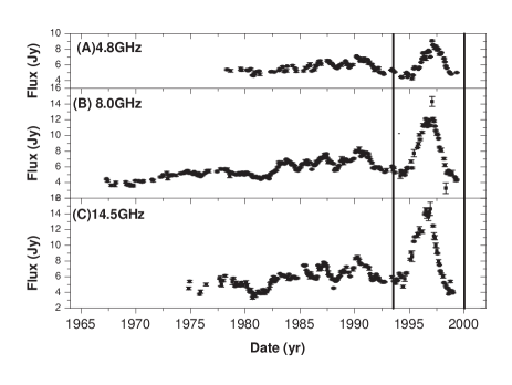
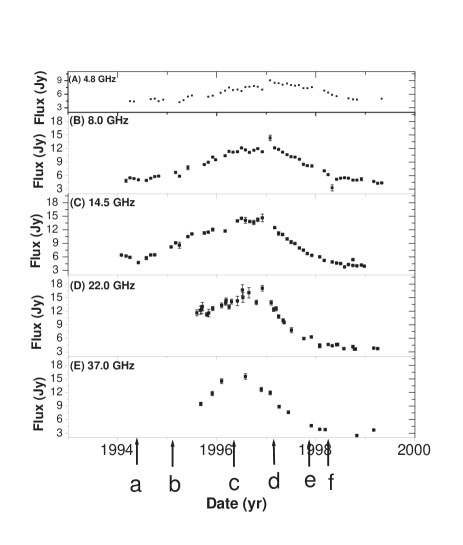
Figure 1: Top: light curves of NRAO 530 at (A)4.8 GHz, (B)8.0 GHz, (C)14.5 GHz from UMRAO (University of Michigan Radio Astronomy Observatory). Bottom: light curves of NRAO 530 observed during the period from 1994 to 1999 at (A)4.8 GHz, (B)8.0 GHz, (C)15.4 GHz from UMRAO and (D)22 GHz, (E)37 GHz from 13.7-meter antenna at Metsahovi Radio Observatory (Teräsranta et al.  Terasranta04 (2004)), arrows with letters a, b, c, d, e and f indicate different epochs plotted in Fig. 6.

2 VLBI Observations and Data Reduction

NRAO 530 was observed at 5, 8, 15, 22 and 43 GHz in February 1997 with the VLBA plus a VLA antenna. It was also observed 3 times in 1999 at 39, 43 and 45 GHz with the VLBA. Detailed parameters of observations can be found in Table 1. The data were recorded in VLBA format with a total bandwidth of 32 MHz (4 IFs) for left circular polarization (LCP) (and also right circular polarization (RCP) in 1997). The observed data were cross-correlated with the VLBA correlator at Socorro, New Mexico of the USA.

Table 1: VLBI Observations of NRAO 530

$\nu$	epoch	integration time	bandwidth	bit rate	polarization(s)	antennas
(GHz)	(year)	(min)	(MHz)	(bit)
(1)	(2)	(3)	(4)	(5)	(6)	(7)
5.0	1997.10	20	32$\times$2	1	RCP, LCP	VLBA+VLA1
8.4	1997.10	20	32$\times$2	1	RCP, LCP	VLBA+VLA1
15.4	1997.12	20	32$\times$2	1	RCP, LCP	VLBA+VLA1
22.2	1997.12	20	32$\times$2	1	RCP, LCP	VLBA+VLA1
43.2	1997.12	20	32$\times$2	2	RCP, LCP	VLBA+VLA1
43.1	1999.32	17	32	2	LCP	VLBA
43.1	1999.40	17	32	2	LCP	VLBA
39.1	1999.42	19	32	2	LCP	VLBA
45.1	1999.42	18	32	2	LCP	VLBA

Notes: (1) Observing frequency in GHz; (2) Observing epoch in yr; (3) Total on-source time in minutes; (4) Recording bandwidth in MHz; (5) sampling rate in bit; (6) Polarization mode, and (7) Observing antennas.

The post-correlation data reduction was carried out using the NRAO AIPS and Caltech DIFMAP packages. We first applied amplitude calibration (at frequencies $\geq$22 GHz atmospheric opacity corrections were made) using the gain curves and system temperatures measured at each station. Then fringe fitting was performed to determine the instrumental delays first, and further to solve for the residual delays, rates and phases. The data were then exported into DIFMAP for self-calibration imaging. These visibilities were time-averaged into 30-second bin with uncertainties estimated from the scatter of data points within the 30 s interval. The data were inspected for obviously bad points, most of which were near the beginning of scan when telescopes were still slewing to the sources. Images were made using the self-calibration and clean procedure for several iterations. A 1-Jy point-source model was employed at the start of each mapping process and the natural weighting of the data was used for all nine images shown in Fig. 2. The detailed paraments of images are summarized in Table 2. For a quantitative analysis of the structure in these images, we did model fits to the calibrated visibility data with elliptical Gaussian components. The results are listed in Table 3. A maximum uncertainty of 15% in the flux density was estimated from the uncertainties of the amplitude calibration and the formal errors of the model fits. The typical uncertainties of the component positions and their sizes were examined to be about 10% of the fitted values. The brightness temperature (column 11 in Table 3) of each component was calculated using the following equation (i.e. Shen et al. Shen97 (1997)),

$$T_{b}=1.22\times 10^{12}S\nu^{-2}(\theta_{maj}\theta_{min})^{-1}(1+z)\leavevmode\nobreak\ K,$$ (1)

where $S$ is the flux density in Jy, $\nu$ the frequency in GHz, z the redshift, $\theta_{maj}$ and $\theta_{min}$ sizes (FWHM) of the major and minor axes in mas, respectively.

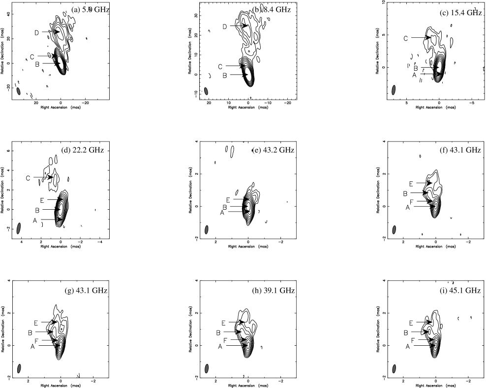
Figure 2: The clean images of NRAO 530 (detailed parameters are listed in Table 2).

Table 2: Descriptions of VLBI images of NRAO 530

	$\nu$	Epoch	Speak	Maj	Min	P.A.	Contours
	(GHz)	(year)	(Jy/beam)	(mas)	(mas)	(deg)	(mJy/beam)
(1)	(2)	(3)	(4)	(5)	(6)	(7)	(8)
(a)	5.0	1997.10	5.7	6.11	2.21	16.1	2.9$\times$(-1,1,2,4,8,16,32,64,128,256)
(b)	8.4	1997.10	7.7	3.80	1.39	15.5	2.8$\times$(-1,1,2,4,8,16,32,64,128,256)
(c)	15.4	1997.12	8.0	1.49	0.49	-8.0	8.4$\times$(-1,1,2,4,8,16,32,64,128,256)
(d)	22.2	1997.12	6.8	1.16	0.32	-9.9	12.7$\times$(-1,1,2,4,8,16,32,64,128,256)
(e)	43.2	1997.12	4.5	0.53	0.19	-7.3	10.0$\times$(-1,1,2,4,8,16,32,64,128,256)
(f)	43.1	1999.32	1.7	0.52	0.19	-8.2	9.7$\times$(-1,1,2,4,8,16,32,64,128)
(g)	43.1	1999.40	1.8	0.55	0.19	-9.0	9.0$\times$(-1,1,2,4,8,16,32,64,128)
(h)	39.1	1999.42	2.0	0.55	0.20	-7.0	10.8$\times$(-1,1,2,4,8,16,32,64,128)
(i)	45.1	1999.42	1.7	0.53	0.19	-8.3	10.2$\times$(-1,1,2,4,8,16,32,64,128)

Notes: (1) Image index (see Fig. 2); (2) Observing frequency; (3) Observing epoch; (4) Peak flux density; (5), (6), (7) Parameters of the restoring Gaussian beam: the full width at half maximum (FWHM) of the major and minor axes and the position angle (P.A.) of the major axis. (8) Contour levels of the image.

Table 3: NRAO 530 model parameters

	$\nu$	Epoch	Component	S	r	$\phi$	$\theta_{maj}$	$\theta_{min}$	P.A.	Tb
	(GHz)	(year)		(Jy)	(mas)	(deg)	(mas)	(mas)	(deg)	(1012K)
(1)	(2)	(3)	(4)	(5)	(6)	(7)	(8)	(9)	(10)	(11)
(a)	5.0	1997.10	B	5.60	0	0	0.78	0.23	24.3	2.9
			C	0.60	4.02	14.7	3.13	1.70	7.8	1.0E-2
			D	0.53	21.92	0.4	16.30	6.12	13.2	4.9E-4
(b)	8.4	1997.10	B	7.73	0	0	0.35	0.21	9.0	3.5
			C	0.64	3.22	12.3	4.07	1.65	20.4	3.1E-3
			D	0.33	22.89	1.1	13.60	5.42	13.9	1.5E-4
(c)	15.4	1997.12	A	0.91	0	0	0.21	0.21	….	2.0E-1
			B	8.01	0.38	16.5	0.22	0.10	48.6	3.66
			C	0.46	3.42	10.2	4.43	1.70	22.4	5.9E-4
(d)	22.2	1997.12	A	1.87	0	0	0.26	0.10	12.0	3.4E-1
			B	6.73	0.29	24.5	0.21	0.16	12.3	9.4E-1
			E	0.12	0.73	8.7	0.14	0.14	…	2.9E-2
			C	0.37	3.24	14.5	4.89	1.68	13.1	2.1E-4
(e)	43.2	1997.12	A	1.62	0	0	0.13	0.04	4.7	3.9E-1
			B	5.76	0.35	21.3	0.17	0.16	-42.3	2.6E-1
			E	0.58	0.53	2.4	0.66	0.28	4.3	3.9E-3
(f)	43.1	1999.32	A	1.63	0	0	0.08	0.05	-0.3	5.1E-1
			F	0.34	0.18	13.4	0.19	0.19	…	1.2E-2
			B	0.28	0.84	27.5	0.59	0.13	27.3	4.6E-3
			E	0.18	1.42	2.8	1.11	0.47	17.7	4.3E-4
(g)	43.1	1999.40	A	1.86	0	0	0.19	0.04	-12.4	3.1E-1
			F	0.22	0.22	20.8	0.13	0.13	…	1.6E-2
			B	0.26	0.85	27.9	0.65	0.18	18.3	2.8E-3
			E	0.22	1.33	2.6	1.22	0.68	19.5	3.3E-4
(h)	39.1	1999.42	A	1.78	0	0	0.07	0.04	10.4	9.6E-1
			F	0.56	0.17	12.2	0.34	0.09	45.5	2.8E-2
			B	0.31	0.92	26.0	0.63	0.20	32.8	3.7E-3
			E	0.21	1.48	2.8	1.24	0.54	23.6	4.8E-4
(i)	45.1	1999.42	A	1.65	0	0	0.12	0.02	-11.2	7.8E-1
			F	0.16	0.19	18.5	0.04	0.04	…	1.1E-1
			B	0.34	0.71	27.4	1.21	0.12	18.3	2.7E-3
			E	0.16	1.29	-1.6	1.33	0.21	11.0	6.5E-4

Note: (1) Index of image (as shown in Fig. 2); (2) Observing frequency; (3) Observing epoch; (4) Component in each image; (5), (6), (7), (8), (9), (10) Model parameters of Gaussian component: S=flux density, r=angular separation and $\phi$=position angle of component with respect to the origin (0,0), full widths at half maximum (FWHM) of the major ($\theta_{maj}$) and minor ($\theta_{min}$) axes and the position angle (P.A.) of the major axis; (11) Brightness temperature.

3 Results

3.1 Components and Their Proper Motions

The source shows different morphologies at different frequencies with more details in the core region revealed at higher frequencies (see Fig. 2). The overall structure is dominated by a compact core plus a jet like feature extending approximately 5 mas from the core along a position angle (P.A.) of 15^∘ which further bends toward the north. Fig. 3 is the projected trajectory based on the locations of the VLBI components in NRAO 530 observed in February 1997, inferring a continuously bending path of the jet emission. Here, we assume the brightest and most compact component A (see Table 3) as the core because it is located at the south end of emission and has the flattest spectral index (see Sect. 3.2). The same core identification is also adopted by Jorstad et al. (Jorstad01 (2001)).

Component D at about 22-23 mas north of the core region was detected at 5 and 8 GHz (Fig. 2 (a) and (b)). This is probably associated with the knot emission, at about 25 mas north of the core, seen from the 1.7 GHz VLBI observations (Bondi et al. Bondi96 (1996)). At about 3-4 mas from the core with a P.A. of 10-15^∘, component C was consistently detected at frequencies of 5, 8, 15 and 22 GHz (Fig. 2 (a), (b), (c) and (d)). This component was also seen by Tingay et al. (Tingay98 (1998)), Shen et al. (Shen97 (1997)) and Jorstad et al. (Jorstad01 (2001)).

The 1997 simultaneous observations at 43, 22 and 15 GHz showed a consistent central core region (Fig. 2 (c), (d) and (e)) which can be fitted with 3 components, A, B and E (Table 3). The fitted relative separations from A component of 0.35 and 0.53 mas for components B and E, respectively at 43 GHz, are in a reasonable agreement with the results from 22 and 15 GHz considering their $>$1 mas angular resolutions (See Table 2). And it is also possible that the $\sim$0.05$-$0.2 mas difference in the measured core separation for components B and E is due to the opacity shift, since the relative separation of VLBI component from the self-absorbed core is frequency dependent. At 15 GHz, component E seemed too weak to be detected (also refer to Fig. 5 for its spectrum). These are comparable to the results obtained from four 43 GHz images at epochs 1995.79 to 1996.90 (Jorstad et al. Jorstad01 (2001)) and 86 GHz image at epoch 1995.38 (Bower et al. Bower97 (1997)). Another four $\sim$43 GHz images (Fig. 2 (f), (g), (h) and (i)) made in April-May 1999 can be well fitted with 4 components: components A, B, E and a new component F at 0.18 mas with P.A. of 25^∘.

By combining our new measurements of angular separations with those published data in 1995 and 1996 (Jorstad et al. Jorstad01 (2001)) of components B and E, we obtain proper motions of 0.21$\pm$0.02 and 0.30$\pm$0.02 mas yr^-1 (Fig. 4), corresponding to superluminal velocities of 10.2$\pm$0.8 c and 14.5$\pm$1.1 c for components B and E, respectively. This infers the ejecting times for components B and E to be around 1995.46 and 1994.76, respectively. These two epochs just fall in the outburst phase shown in Fig. 1 (also see discussion in Sect. 3.3). EGRET reported the increasing $\gamma$-ray flux densities from the direction of NRAO 530 during two periods (1994.2-1994.6 and 1995.4-1995.5) with the average fluxes of 64$\pm$26 pJy and 127$\pm$48 pJy (Hartman et al. hartman99 (1999)). As EGRET could not observe NRAO 530 with dense time sampling and long integrations, the $\gamma$-ray measurements have large uncertainties and can not rule out that $\gamma$-ray flares were missed or that maximum of an ongoing flare was really seen. According to the existing data (VLBA and EGRET) of NRAO 530 we think that the emergence of components B and E are closely following the $\gamma$-ray flares in NRAO 530. Activity of $\gamma$-ray has been found to be correlated with infrared to X-ray activity in 3C 279 (Maraschi et al. Maraschi94 (1994)) and, to occur before or during a radio and millimeter outburst in many sources (Reich et al. Reich93 (1993)).

For component C, we also plot its separation from the core (Fig. 4) as a function of time measured in 1992, 1995, 1996 and 1997 by Shen et al. (Shen97 (1997)), Jorstad et al. (Jorstad01 (2001)), Bower and Backer (Bower98 (1998)) and us (this work), respectively. The best fitted proper motion is about $-0.01\pm$0.13 mas yr^-1, corresponding to an apparent velocity of $-0.35\pm$6.04 c. This is quite different from the apparent velocity of 29$\pm$9$h^{-1}$c (Hubble constant H₀=100 h km s^-1 Mpc^-1, deceleration parameter q₀=0.1, and cosmological constant $\Lambda=0$) reported by Jorstad et al. (Jorstad01 (2001)) (component D in their paper). Our new estimate with more time coverage in data indicates that there is no appreciable motion for component C. The previously reported large apparent velocity of 29$\pm$9$h^{-1}$c may be due to their limited epochs of data and thus the large uncertainty. This discrepancy may be related to the complex structure in component C (Fig. 2(c) and (d)), which results in a large error in the determination of its position. Such kind of diffused morphology could be due to internal jet structure, blending effects of shocks or some sort of interaction. For the reason to be discussed in Sect. 4, we think it is mainly caused by the interaction of jet emission with the surrounding medium.

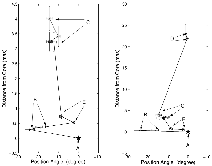
Figure 3: The projected trajectory of jet components observed in 1997: (Left) within central 4 mas, (Right) within 20 mas, showing a continuously bending jet moving away from the central core. A, B, E, C and D represent different VLBI components and the solid lines are connections of individual jet components.

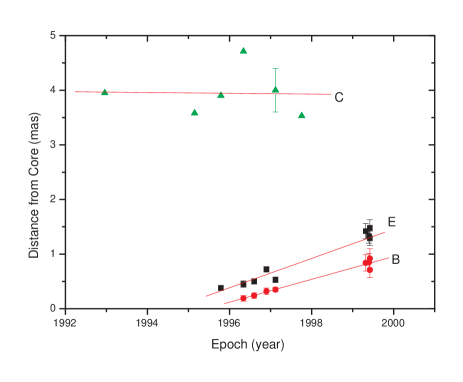
Figure 4: Separation of components B, E and C from the assumed core component A as the function of the observing epoch.

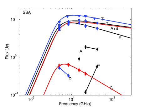
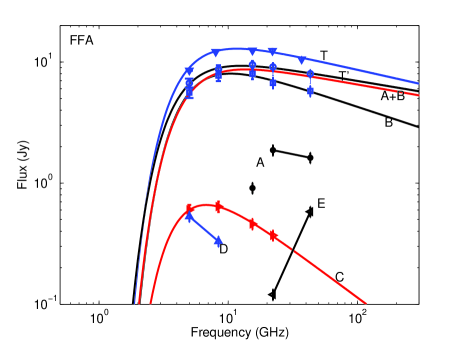
Figure 5: Components spectral fit of NRAO 530 in February 1997 (top: spectra are fit with the SSA, bottom: spectra are fit with the FFA

Table 4: Spectral fitting results with the SSA and FFA

Parameters	SSA			FFA
	B	C	A+B		B	C	A+B
$\alpha$	0.31	0.64	0.14		0.35	0.79	0.19
$S_{0}$(Jy)	0.12	0.02	0.13		21.77	4.38	15.59
$\tau$	148.31	159.90	101.40		23.33	20.88	21.89

3.2 Components’ Spectra

For the quasi-simultaneous observations in February 1997, the spectra of VLBI components (A, B, C and D) can be fit with $S_{\nu}\propto\nu^{-\alpha}$ and the resultant optically thin spectral indexes are $\alpha_{A}$=0.21, $\alpha_{B}$=0.31$\pm$0.07, $\alpha_{C}$=0.58$\pm$0.01 and $\alpha_{D}$=0.91. Component A is regarded as the core of NRAO 530 since it has the flattest spectral index and it is at the south end of the overall emission. Component E seems to show an inverted spectrum with a high turnover frequency (greater than 43 GHz) in 1997. This is likely to be due to the strong variability at 43 GHz as 1999 data had a three times lower flux density. The fitted two-point spectral index is $\alpha_{E}$=$-$1.5 between 22 and 43 GHz.

In order to discuss the possibly dominant mechanism for the observed low frequency absorption in components B and C, both the synchrotron self-absorption (SSA) and the free-free absorption (FFA) are tried to fit the convex spectra with the following formulae,

$$S_{\nu}=S_{0}\nu^{2.5}[1-{\rm exp}(-\tau_{s}\nu^{-\alpha-2.5})]$$ (2)

for the SSA and,

$$S_{\nu}=S_{0}\nu^{-\alpha}{\rm exp}(-\tau_{f}\nu^{-2.1})$$ (3)

for the FFA, where $\nu$ is the observing frequency in GHz, $S_{0}$ is the intrinsic flux density at 1 GHz in Jy, $\tau_{f}$ and $\tau_{s}$ are the SSA and FFA coefficients at 1 GHz, respectively. We also performed the fits to the combined component (A+B) emission, which is believed to be represented by component B at low frequencies (5 and 8 GHz) due to the limited resolutions (see Table 3) and is resolved out at frequencies $\geq$15 GHz. All the fitting results are listed in Table 4 with the fitting curves shown in Fig. 5.

Both the SSA and FFA fit the spectra of components B and C equally well. Thus, the spectral fit itself is not adequate to tell which mechanism is mainly responsible for the absorption towards components B and C. However, a short synchrotron cooling timescale seems to suggest that FFA plays an important role in component C (see Sect. 4). If so, that the FFA coefficients for components B and C are almost the same (see Table 4) infers the presence of the FFA by the same surrounding medium in component B. Then, one could estimate that the absorbing material should cover at least about 25 pc in size to produce the same FFA towards components B and C which were separated by about 3 mas in the sky in 1997. The interaction of the surrounding interstellar medium causing FFA with the jet emission in NRAO 530 can be used to explain the poorly determined proper motion in component C (see Sect. 3.1).

For comparison, we also plotted the spectrum of the sum of all the VLBI components (labelled by T^′ in Fig. 5) as well as the spectrum from single dish data (labelled by T in Fig. 5). The missing of flux density is persistently seen in all five VLBI frequencies. This is likely due to the effect of the resolution of the extended components. Therefore our amplitude calibrations, including the atmospheric opacity corrections, should be reasonable.

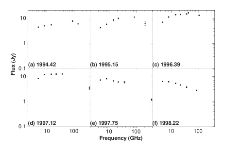
Figure 6: Spectral variability seen in a flare from 1994.5 to 1998.5. Flux densities at 43, 86, 88, 95, 107, 142, 150, 215 and 375 GHz are listed in (Table 5). Letters a, b, c, d, e, f represent different epochs indicated in Fig. 1.

3.3 Spectral Variability

A complete outburst profile can be traced from mid-1994 to mid-1998 (between two vertical lines in Fig. 1 (Top)). To analyze spectral variability during this radio outburst we select six epochs: 1994.42 (a), 1995.18 (b), 1996.39 (c), 1997.12 (d), 1997.75 (e) and 1998.22 (f). Fig. 6 shows the spectral distribution at these six epochs based on the data points in Fig. 1 (at frequencies $\leq$ 37.0 GHz) and in Table 5 (at frequencies $\geq$ 43 GHz). It is quite clear in Fig. 6 that the turnover frequency is increasing during the rising phase (represented by epochs (a), (b) and (c)) when the flux density is increasing (see Fig. 1).

From 1997.12 (d) the turnover frequency starts to decrease when the total flux density decreases. This is because that high frequency photons lose energy quickly with jet expanding and thus the flux density at high frequency decrease too. In 1998.22 (f) the spectrum returns to the level of quiescent phase.

Table 5: Total Flux density data of NRAO 530 at $\nu\geq 43$ GHz

$\nu$	epoch	flux	error	references
(GHz)	(Year)	(Jy)	(Jy)
43	1996.39	16.6	0.5	Falcke et al. Falcke98 (1998)
86	1995.18	11.2	0.3	Krichbaum et al. Krichbaum97 (1997)
88	1994.42	7.8	0.5	Reuter et al. Reuter97 (1997)
95	1996.82	12.6	0.7	Falcke et al. Falcke98 (1998)
107	1996.39	13.2	0.4	Falcke et al. Falcke98 (1998)
142	1994.42	6.0	0.5	Reuter et al. Reuter97 (1997)
150	1996.82	12.0	1.2	Falcke et al. Falcke98 (1998)
215	1995.18	6.2	1.1	Krichbaum et al. Krichbaum97 (1997)
375	1997.12	3.5	0.5	Robson et al. Robson01 (2001)
375	1997.26	2.7	0.3	Robson et al. Robson01 (2001)
375	1997.75	1.2	0.1	Robson et al. Robson01 (2001)

4 Discussion

It is well known that the observed transverse velocity ($\beta_{app}=v_{app}/c$, $v_{app}$ the apparent velocity) is related to the true velocity ($\beta$) and the angle to the line of sight ($\theta$) by $\beta_{app}=\beta\sin\theta/(1-\beta\cos\theta)$. Therefore, the maximum angle ($\theta$) of 11.2^∘ and 7.9^∘ for components B and E can be estimated from their corresponding apparent velocities of 10.2 c and 14.5 c.

Doppler factor ($\delta$) is defined as $\delta=\Gamma^{-1}(1-\beta\cos\theta)^{-1}$, where $\Gamma=(1-\beta^{2})^{-1/2}$ is the Lorentz factor. By means of the above expression of $\beta_{app}$, we can derive $\delta=\Gamma\pm(\Gamma^{2}-\beta_{app}^{2}-1)^{1/2}$. Then the Doppler factor of component B is $\delta=\Gamma_{min}=10.2$ when the Lorentz factor is $\Gamma_{min}=(1+\beta_{app}^{2})^{1/2}$. In the same way we compute the Doppler factor of another superluminal jet component E, $\delta=14.5$.

For another scenario in which no intrinsic acceleration or deceleration happened in the jet motion, i.e., jets are ejected with a same velocity $\beta$ (or a constant Lorentz factor $\Gamma$), the changes of apparent velocities would be mainly due to different viewing angles (variable $\theta$). The observed fastest apparent speed of 14.5c (for component E) in NRAO 530 will limit the constant Lorentz factor to be at least of 14.5, and thus we use $\Gamma_{\rm min}=15$. Combining with the apparent velocity measurements, we can obtain the viewing angles of $9.7^{\circ}$ and 1.6^∘ for component B with $\beta_{app}=10.2\rm c$, and $4.9^{\circ}$ and 3.0^∘ for component E with $\beta_{app}=14.5\rm c$. The corresponding Doppler factors are 4.0 and 26.0 for component B, and 11.3 and 18.7 for component E.

Estimates of the magnetic field in a radio source can be obtained in two distinct ways. Firstly, by assuming the equipartition of energy between the particles and the magnetic field, one can have (e.g., Pacholczyk pacholczyk70 (1970))

$$B^{\rm eq}=[4.5(1+k)f(\alpha,\nu_{1},\nu_{2})LR^{-3}]^{2/7}\leavevmode\nobreak\ ,$$ (4)

where B^eq in G is the magnetic field when the total energy of magnetic field and particles has a minimum value (equipartition between the energy of the particles and the energy of the magnetic field), k is the energy ratio between the heavy particles and the electrons (we used k=100), $f(\alpha,\nu_{1},\nu_{2}$) is tabulated in Appendix 2 of Pacholczyk (pacholczyk70 (1970)), $\alpha$ is the optically thin spectral index, $\nu_{1}$ and $\nu_{2}$ are the lower and upper cutoff frequencies of the synchrotron spectrum with typical values of 10⁷ and 10¹¹ Hz, $R=\frac{d_{L}\Theta}{2(1+z)}$ is the radius of component in cm (here, $\Theta$ is the angular diameter and d_L is luminosity distance), L is the synchrotron luminosity in erg s^-1 and can be expressed as L$=4\pi$$d_{L}^{2}\int_{\nu_{1}}^{\nu_{2}}S_{\nu}d\nu$ (here, S_ν is flux density at a frequency $\nu$). It should be mentioned that B^eq is insensitive to the values of $k$ and the fraction of the source’s volume occupied by the magnetic field and the particles which is auusmed to be 1. By assuming $\int_{\nu_{1}}^{\nu_{2}}S_{\nu}d\nu\simeq S_{m}\nu_{m}$, we can re-write

$$B^{eq}\simeq 4.0\times 10^{-4}[f(\alpha,10^{7},10^{11})(1+z)^{3}d_{L}^{-1}\Theta^{-3}S_{m}\nu_{m}]^{2/7}\leavevmode\nobreak\ ,$$ (5)

where $\nu_{m}$ is the turnover frequency in GHz, $S_{m}$ is the extrapolated optically thin flux density at the turnover frequency in Jy, and luminosity distance $d_{L}$ and angular diameter $\Theta$ are in Gpc and mas, respectively.

Secondly, assuming that the inverted spectrum is due to SSA, one can estimate the magnetic field (i.e., Marscher Marscher83 (1983)),

$$B^{syn}=10^{-5}b(\alpha)\Theta^{4}\nu^{5}_{m}S^{-2}_{m}\delta/(1+z)$$ (6)

where $B^{syn}$ is the magnetic field in G, and b($\alpha$) is a tabulated parameter dependent on the spectral index $\alpha$ (Table 1 in Marscher (Marscher83 (1983))). For component B, $\alpha$=0.31 gives b(0.31)$\approx$3.0.

From the SSA spectral fitting results for component B ($\Theta$=$\sqrt{\theta_{maj}\times\theta_{min}}$=0.2 mas, S_m=8 Jy, $\nu_{m}$=10 GHz) and $\delta=$1 (without consideration of relativistically beaming effect), we obtained B${}_{B}^{eq}\simeq 580$ mG and $B_{B}^{syn}\simeq 4\times 10^{-2}$ mG. The time scale for an electron to lose its energy through synchrotron radiation is $t_{1/2}\simeq 2.76\times 10^{4}\leavevmode\nobreak\ ({\rm yr})\leavevmode\nobreak\ (\frac{B^{syn}}{\rm 1\leavevmode\nobreak\ mG})^{-1.5}(\frac{\nu_{m}}{\rm 1\leavevmode\nobreak\ GHz})^{-0.5}$. This gives a cooling time scale of $1.1\times 10^{6}$ yr for component B, while the intrinsic cooling time scale in the source rest frame should be greater when Doppler factor is larger than (1+z). In the same way, we computed the magnetic field for component A, $B_{A}^{eq}\simeq$560 mG and B${}_{A}^{syn}\simeq 8$ mG with S_m=1.87 Jy, $\nu_{m}$=22.2 GHz, $\Theta$=0.16 mas, $\alpha$=0.21 and $\delta$=1 since it seems to have a (presumably synchrotron self-absorbed) inverted spectrum at frequencies between 15 and 22 GHz (see Fig. 5).

The ratio of the particle energy density ($u_{p}$) to the energy density of the magnetic field ($u_{m}$) can be expressed as (i.e., Readhead readhead94 (1994)) $\frac{u_{p}}{u_{m}}=(\frac{B^{eq}}{B^{syn}})^{17/4}$. We get $\frac{u_{p}}{u_{m}}\simeq 6.9\times 10^{7}$ and $\frac{u_{p}}{u_{m}}\simeq 5.5\times 10^{17}$ for component A and B, implying that both components A and B are particle dominated or that their emissions are relativistically beamed. In the former case, for component B this high ratio may account for the observed fast decrease in the radio flux density (from 5.76 Jy to $\sim$0.3 Jy) in two years even though its synchrotron cooling time could be much longer ($\simeq 1.1\times 10^{6}$ yr). This is because that the high ratio of particle to magnetic field energies may cause the inverse Compton catastrophe (Readhead readhead94 (1994)) and, inverse Compton scattering of X-ray photons may further result in the $\gamma$-ray emission (e.g., Hartman et al. hartman92 (1992)).

In the latter case, as the equations for the magnetic field (equations (5) and (6)) have different dependencies on the Doppler boosting factor, thus we can obtain

$$\frac{B^{eq}}{B^{syn}}\simeq(\frac{B_{int}^{eq}}{B_{int}^{syn}})(\frac{\delta}{1+z})^{6+\frac{16\alpha}{7}}\leavevmode\nobreak\ \leavevmode\nobreak\ \leavevmode\nobreak\ ,$$ (7)

where $B^{eq}$ and $B^{syn}$ are the measured magnetic field, $B_{int}^{eq}$ and $B_{int}^{syn}$ are the magnetic field estimated in the source rest frame. When $B_{int}^{eq}\simeq B_{int}^{syn}$, the Doppler factor in equation (7) is defined as the equipartition Doppler-factor, $\delta^{eq}$. To derive equation (7), we have used the following relations, $\nu^{ob}_{m}=(\frac{\delta^{eq}}{1+z})\nu^{\prime}_{m}$, $S^{ob}_{m}=(\frac{\delta^{eq}}{1+z})^{3+\alpha}S^{\prime}_{m}$ and $\Theta^{ob}=(\frac{1+z}{\delta^{eq}})\Theta^{\prime}$ (Singal and Gopal-Krishna singal85), here $\Theta^{ob}$, $\nu^{ob}_{m}$ and $S^{ob}_{m}$ are angular diameter, inverted frequency and corresponding flux density in the observer’s frame, respectively, and $\Theta^{\prime}$, $\nu^{\prime}_{m}$ and $S^{\prime}_{m}$ in the source rest frame. Then we got the equipartition Doppler-factors for components A and B of $\delta^{eq}_{A}\simeq 3.7$ and $\delta^{eq}_{B}\simeq 7.2$, respectively. These are comparable to the equipartition Doppler factors of 7.0 at 10 GHz (Marscher et al. marscher77 (1977)) and 5.2 at 15 GHz (Güijosa and Daly guijosa96 (1996)).

Similarly, for component C we estimate $B_{C}^{eq}\simeq 36$ mG, $B_{C}^{syn}\simeq 29\times 10^{3}$ mG, $u_{p}/u_{m}\simeq 7.4\times 10^{-13}$, $\delta^{eq}_{C}\simeq 0.8$ and the synchrotron cooling time of $\sim$0.8 day, with the following parameters: S_m=0.65 Jy, $\nu_{m}$=7 GHz, $\Theta$=2.5 mas, $\alpha$=0.53 and $\delta$=1.0. As the magnetic field is strongly dependent on measured component parameters, the high magnetic field of component C may be due to its large size ($\sim 2.5$ mas). Assuming that the equipartition is maintained in component C, we can estimate a size scale of 0.64 mas for component C so that both the calculated $B_{C}^{eq}$ and $B^{syn}_{C}$ are equal to 120 mG. The resultant synchrotron cooling time would be 7.6 yr, still too short for the SSA model. So, it is very likely that the FFA of the surrounding medium dominates the observed absorption in component though we cannot completely rule out the SSA effect.

As the Doppler-factors of jets are expected to increase with decreasing viewing angle for the assumed constant Lorentz factor, the equipartition Doppler-factors also should decrease systematically along a bent jet given that the viewing angle is increasing monotonically along the bending trajectory. This is probably the reason that the $\delta_{eq}$ of component C is smaller than the values of components A and B. However, the fact of $\delta^{eq}_{B}>\delta^{eq}_{A}$ is consistent with that component B is brighter than component A in 1997. For component B, the Doppler-factor estimated from $\beta_{app}$ of $\delta=\Gamma_{min}=10.2$ is comparable to the equipartition Doppler-factor $\delta^{eq}_{B}\simeq 7.2$, suggesting that most likely jets have the minimum Lorentz factors in an equivalent state. For component C, there is no appreciable proper motion (Section 3.1), which suggests a Doppler-factor of $\sim$1.0 ($\delta=\Gamma_{min}=\sqrt{1+\beta_{app}^{2}}$). This is consistent with the estimated equipartition Doppler-factor of 0.8, inferring that it approaches energy equivalent state between particle and magnetic field in the source rest frame. The fact that $\delta^{eq}_{C}\simeq 0.8$ is smaller than 1+z=1.902 for component C in NRAO 530 implies that it is Hobble flow that results in the observed departure from the energy equipartition in component C.

5 Summary

We presented the high-resolution VLBI images of NRAO 530 made at 5, 8, 15, 22, 39, 43, 45 GHz in 1997 and 1999. Combining our new measurements with the past data we estimated superluminal motions of components B and E at apparent velocities of 10.2 c and 14.5 c, respectively. These are consistent with that components B and E were ejected in 1995.46 and 1994.76 following the $\gamma$-ray flares of 127 and 64 pJy, respectively. Flat spectra are seen in central two components (A and B), and the most compact component A with the flattest spectral index at the south end is identified as the core. We derive the equipartition Doppler-factor based on the equations of (5) and (6), and obtain $\delta^{eq}$s of 3.7, 7.2 and 0.8 for components A, B and C, respectively. These are consistent with a larger flux density in component B, the non-detection of proper motion in component C and a bent jet. The synchrotron cooling timescale argues that the FFA is responsible for the inverted spectrum of component C though the SSA effect can not be completely ruled out yet. While for component B both the SSA and FFA could play a role, we propose that the FFA may be at work given that almost the same FFA coefficients were fitted for both components B and C. If so, the absorbing material would have a projected size of at least 25 pc.

- (1) Aller, H. D., Aller, M. F., Latimer, G. E., and Hodge, P. E. 1985, ApJS, 59, 513
- (2) Bondi, M., et al. 1996, A&A, 308, 415
- (3) Bower, G. C., Backer, D. C., Wright, M., and Forster, J. R. 1997, ApJ, 484, 118
- (4) Bower, G. C., and Backer, D. C. 1998, ApJ, 507, 117
- (5) Falcke, H., Goss, W. M., Matsuo, H., Teuben, P., and Zhao, J- H. 1998, ApJ, 499, 731
- (6) Güijosa, A., and Daly, R. A. 1996, ApJ, 461, 600
- (7) Hartman, R. C., et al. 1992, ApJ, 385, 1
- (8) Hartman, R. C., et al. 1999, ApJS, 123, 79
- (9) Jorstad, S. G., Marscher, A. P., Mattox, J. R., Wehrle, E., Bloom, S. D., and Yurchenko, A. V. 2001, ApJS, 134, 181
- (10) Junkkarinen, V. 1984, PASP, 96, 539
- (11) Krichbaum, T. P., et al. 1997, A&A, 323, 17
- (12) Maraschi, L., et al. 1994, ApJ, 435, 91
- (13) Marscher, A. P., et al. 1977, ApJ,233, 498
- (14) Marscher, A. P., and Marshall, F. E. 1979, ApJ, 233, 498
- (15) Marscher, A. P., and Broderick, J. J. 1981, ApJ, 249, 406
- (16) Marscher, A. P. 1983, ApJ, 264, 296
- (17) Medd, W. J., Andrew, B. H., Harvey, G. A., and Locke, J. L. 1972, MNRAS, 77, 109
- (18) Pacholczyk, A. G. 1970, Radio astrophysics (San Francisco:Freeman), 97
- (19) Pollock, J. T., Pica, A. J., Smith, A. G., Leacock, R. J., Edwards, P. L., and Scott, R. L. 1979, AJ, 84, 1658
- (20) Readhead, A. C. 1994, ApJ, 624, 51
- (21) Reich, W., et al. 1993, A&A, 273, 65
- (22) Reuter, H. P., et al. 1997, A&AS, 122, 271
- (23) Robson, E. I., Stevens, J. A., and Jenness, T. 2001, MNRAS, 327, 751
- (24) Shen, Z. -Q., et al. 1997, AJ, 114, 1196
- (25) Teräsranta, H., et al. 2004, A&A, 427, 769
- (26) Tingay, S. J., Murphy, D. W., and Edwards, P. G. 1998 ApJ, 500, 673
- (27) Welch, W. J., and Spinrad, H. 1973, PASP, 85, 456