The Theory of Bodily Tides.
The Models and the Physics

Abstract

Description of tides is based on the form of dependence of the geometric lag $\delta_{1}$ on the tidal-flexure frequency $\chi$. Some authors put $\delta_{1}\sim\chi^{0}$, others set $\delta_{1}\sim\chi^{1}$. The actual dependence of the lag on the frequency is complicated and determined by the planet’s rheology. A particular form of this dependence will fix the form of the frequency dependence of the tidal quality factor $\,Q\,$. Since at present we know the shape of the function $Q(\chi)$, we can reverse our line of reasoning and obtain the appropriate frequency-dependence of the lag. Employment of a realistic dependency $Q(\chi)$ renders considerable changes in the timescales defined by tidal dynamics.

1 The Singer-Mignard theory of bodily tides

The earliest efforts aimed at modeling bodily tides were undertaken in the end of the XIX^th century by Darwin (1879, 1880). A much simplified theory was later offered by MacDonald (1964) who assumed the geometric lag angle to be a fixed constant. With the latter assumption regarded as a critical deficiency, his theory soon fell into disuse in favour of the approach by Singer and Mignard. Singer (1968) suggested that the subtended angle should be proportional to the principal frequency $\chi$ of the tide. This was equivalent to setting $\Delta t$ constant in (2 - 3). Singer applied this new theory to the Moon and to Phobos and Deimos. A detailed mathematical development of Singer’s idea can be found in Mignard (1979, 1980) who completely avoided using the lag angle and operated only with the position and time lags. Later, Singer’s assumption of a constant $\,\Delta t\,$ was employed also by Touma & Wisdom (1994) and Peale & Lee (2000).

A far more comprehensive theory was developed by Kaula (1964). While Kaula assumed the lag angle and the quality factor to be frequency-independent constants, his approach was general enough to embrace an arbitrary frequency-dependence of these parameters. This way, it enables one to employ an arbitrary rheology, i.e., to assume that different tidal modes fall behind the appropriate modes of the perturbing potential with different phases and, accordingly, with difference geometric lag angles.

In the special case of all tidal modes lagging by the same time delay $\,\Delta t\,$, one can model a dynamical tide with a static tide where all the time-dependent variables are shifted back by $\,\Delta t\,$. This gives birth to the concept of a fictitious satellite.

If the actual satellite is located at a planetocentric position $\vec{r}$, it generates a tidal bulge that either advances or retards the satellite motion, depending on the interrelation between the planetary spin rate $\omega_{p}$ and the tangential part of satellite’s velocity $\vec{v}$ divided by $r\equiv|\mbox{{\boldmath$\vec{r}$}}|$. It is convenient to imagine that the bulge emerges beneath a fictitious satellite located at

$$\mbox{{\boldmath$\vec{r}$}}_{f}\,=\,\mbox{{\boldmath$\vec{r}$}}\,+\,\mbox{\boldmath$\vec{\boldmath{\,f}}$}\;\;\;,$$ (1)

where the position lag  $\vec{\boldmath{\,f}}$  is given by

$${\vec{\mbox{\it{f}}}}\;=\;\Delta t\;\left(\;\mbox{{\boldmath$\vec{\omega}$}}_{p}\times\mbox{{\boldmath$\vec{r}$}}\;-\;\mbox{{\boldmath$\vec{v}$}}\;\right)\;\;\;,$$ (2)

$\Delta t\,$ being the time lag between the real and fictitious tide-generating satellites. For vanishing eccentricity and inclination, the quantity

$$\delta\;\equiv\;\frac{|\mbox{\boldmath$\vec{\boldmath{\,f}}$}|}{r}\;=\;\frac{\Delta t}{r}\;|\mbox{{\boldmath$\vec{\omega}$}}_{p}\times\mbox{{\boldmath$\vec{r}$}}\;-\;\mbox{{\boldmath$\vec{v}$}}|\;\;\;.$$ (3)

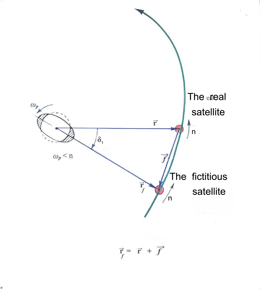
Figure 1: The position lag  $\vec{f}$  and the angular lag $\,\delta_{1}\,$ of a satellite located below the synchronous orbit. (For a moon located above the synchronous orbit both lags will be pointing in an opposite direction.) Be mindful that $\,\delta\,$ defined through (3) does not coincide with the subtended angle $\,\delta_{1}\,$, except for circular orbits.

coincides with the absolute value of the angle $\,\delta_{1}\,$ subtended at the planet’s centre between the satellite and the tidal bulge, as on Fig. 1. For non-circular orbits, they differ.

The imaginary satellite is merely a way of illustrating the time lag between the tide-raising potential and the distortion of the body. This concept implies no new physics, and is but a convenient figure of speech employed to express the fact that at each instance of time the dynamical tide is modeled with a static tide where all the time-dependent variables are shifted back by $\,\Delta t\,$, i.e., (a) the moon is rotated back by $\,\mbox{{\boldmath$\vec{v}$}}\,\Delta t\,$, and (b) the attitude of the planet is rotated back by $\,\mbox{{\boldmath$\vec{\omega}$}}_{p}\,\Delta t\,$. From the viewpoint of a planet-based observer, this means that a dynamical response to a satellite located at  $\vec{r}$  is modelled with a static response to a satellite located at $\,\mbox{{\boldmath$\vec{r}$}}_{f}\,\equiv\,\mbox{{\boldmath$\vec{r}$}}\,-\,\Delta t\,(\mbox{{\boldmath$\vec{v}$}}\,-\,\mbox{{\boldmath$\vec{\omega}$}}_{p}\times\mbox{{\boldmath$\vec{r}$}})\,$.

It should be reiterated that the simplistic concept of a fictitious satellite can be used only for an equatorial circular orbit, within the Singer-Mignard model (the latter implying that all tidal modes get delayed by the same time lag $\,\Delta t\,$).

Delayed response means lagging both in the location of the bulge and in its height (compared to the height of a static bulge). The well-known relation $\;1/Q\,=\,\tan 2\delta_{1}\;$ interconnects the quality factor with the “tangential lag” $\,\delta_{1}\,$ (see the Appendix), while the magnitude lagging is taken care of by the frequency-dependence of the Love number.

2 The tidal frequency $\chi$ and the quality factor $Q$

2.1 The principal tidal frequency

The principal frequency of tidal flexure is $\,2\,|n-\omega_{p}|\,$, where $\,n\,$ and $\omega_{p}\equiv|\,\mbox{{\boldmath$\vec{\omega}$}}_{p}|$ stand for the satellite’s mean motion and the planet’s spin rate.

For an equatorial circular orbit, the satellite velocity relative to the surface is

$$|\,\mbox{{\boldmath$\vec{\omega}$}}_{p}\times\mbox{{\boldmath$\vec{r}$}}~{}-~{}\mbox{{\boldmath$\vec{v}$}}\,|~{}=\;r\;|\,\omega_{p}\,-\,n\,|\;\;\;,$$ (4)

the tidal frequency being

$$\chi\;=\;2\;|\,\omega_{p}\,-\,n\,|\;\;\;\;,$$ (5)

and the angular lag being

$$\delta\;\equiv\;\frac{\Delta t}{r}\;|\,\mbox{{\boldmath$\vec{\omega}$}}_{p}\times\mbox{{\boldmath$\vec{r}$}}\;-\;\mbox{{\boldmath$\vec{v}$}}\,|\;=\;\frac{\Delta t}{2}\;\chi\;\;\;.$$ (6)

While in this particular case we have only the principal tidal mode, in the generic case (when $\,{\it{i}}\,$ or $\,e\,$ is not small, or when $\,\Delta t\,$ is frequency-dependent) an infinite spectrum of tidal modes will emerge.

2.2 Goldreich’s admonition:
a general difficulty stemming from nonlinearity

Darwin (1908), Jeffreys (1961), Kaula (1964) and other authors always started with the fact that each elementary volume of the planet is subject to a tide-raising potential, which in general is not periodic but can be expanded into a sum of periodic terms. They then employed the linear approximation introduced by Love, according to which the tidal perturbations of the potential yield linear response of the shape and linear variations of the stress. Within the linear approximation, the overall dissipation inside the planet may be represented as a sum of attenuation rates corresponding to each periodic disturbance:

$$\langle\,\dot{E}\;\rangle\;=\;\sum_{i}\;\langle\,\dot{E}(\chi_{\textstyle{{}_{i}}})\;\rangle$$ (7)

where, at each frequency $\,\chi_{i}\,$,

$$\langle\,\dot{E}(\chi_{\textstyle{{}_{i}}})~{}\rangle~{}=~{}-~{}2~{}\chi_{\textstyle{{}_{i}}}~{}\frac{\,\langle\,E(\chi_{\textstyle{{}_{i}}})~{}\rangle\,}{Q(\chi_{\textstyle{{}_{i}}})}~{}=\,\;-\;\chi_{\textstyle{{}_{i}}}\;\frac{\,E_{{}_{peak}}(\chi_{\textstyle{{}_{i}}})\,}{Q(\chi_{\textstyle{{}_{i}}})}\;\;\;,$$ (8)

$\langle\,.\,.\,.\,\rangle~{}$ standing for averaging over flexure cycle, $\,E(\chi_{\textstyle{{}_{i}}})\,$ denoting the energy of deformation at the frequency $\,\chi_{\textstyle{{}_{i}}}\,$, and $Q(\chi_{\textstyle{{}_{i}}})\,$ being the quality factor of the material at this frequency. Introduced empirically as a means to figleaf our lack of knowledge of the attenuation process in its full complexity, the notion of $\,Q\,$ has proven to be practical due to its smooth and universal dependence upon the frequency and temperature. At the same time, this empirical treatment has its predicaments and limitations. Its major inborn defect was brought to light by Peter Goldreich who pointed out that the attenuation rate at a particular frequency depends not only upon the appropriate Fourier component of the stress, but also upon the overall stress. This happens because for real minerals each quality factor $\,Q(\chi_{\textstyle{{}_{i}}})\,$ bears dependence not only on the frequency $\,\chi_{\textstyle{{}_{i}}}\,$, but also on the $\,\chi_{\textstyle{{}_{i}}}\,$ component of the stress and, most importantly, also on the overall stress. This, often-neglected, manifestation of nonlinearity may be tolerated only when the amplitudes of different harmonics of stress are comparable. However, when the amplitude of the principal mode is orders of magnitude higher than that of the harmonics (tides being the case), then the principal mode will, through this nonlinearity, make questionable our entire ability to decompose the overall attenuation into a sum over frequencies. Stated differently, the quality factors corresponding to the weak harmonics will no longer be well defined physical parameters.

Here follows a quotation from Goldreich (1963):
“… Darwin and Jeffreys both wrote the tide-raising potential as the sum of periodic potentials. They then proceeded to consider the response of the planet to each of the potentials separately. At first glance this might seem proper since the tidal strains are very small and should add linearly. The stumbling block in this procedure, however, is the amplitude dependence of the specific dissipation function. In the case of the Earth, it has been shown by direct measurement that $\,Q\,$ varies by an order of magnitude if we compare the tide of frequency $\,2\omega-2n\,$ with the tides of frequencies $\,2\omega-n\,$, $\,2\omega-3n\,$, and $\,\frac{\textstyle 3}{\textstyle 2}n\,$. This is because these latter tides have amplitudes which are smaller than the principle tide (of frequency $\,2\omega-2n\,$ ) by a factor of eccentricity or about 0.05. It may still appear that we can allow for this amplitude dependence of Q merely by adopting an amplitude dependence for the phase lags of the different tides. Unfortunately, this is really not sufficient since a tide of small amplitude will have a phase lag which increases when its peak is reinforcing the peak of the tide of the major amplitude. This non-linear behaviour cannot be treated in detail since very little is known about the response of the planets to tidal forces, except for the Earth.”

On these grounds, Goldreich concluded the paragraph with an important warning that we “use the language of linear tidal theory, but we must keep in mind that our numbers are really only parametric fits to a non-linear problem.”

In order to mark the line beyond which this caveat cannot be ignored, let us first of all recall that the linear approximation remains applicable insofar as the strains do not approach the nonlinearity threshold, which for most minerals is of order $\,10^{-6}\,$. On approach to that threshold, the quality factors may become dependent upon the strain magnitude. In other words, in an attempt to extend the expansion (7 - 8) to the nonlinear case, we shall have to introduce, instead of $\,Q(\chi_{\textstyle{{}_{i}}})\,$, some new functions $\,Q(\,\chi_{\textstyle{{}_{i}}}\,,\;E_{{}_{peak}}(\chi_{\textstyle{{}_{i}}})\,,\;E_{{}_{overall}}\,)\;$. (Another complication is that in the nonlinear regime new frequencies will be generated, but we shall not go there.) Now consider a superposition of two forcing stresses – one at the frequency $\,\chi_{\textstyle{{}_{1}}}\,$ and another at $\,\chi_{\textstyle{{}_{2}}}\,$. Let the amplitude $\;E_{{}_{peak}}(\chi_{\textstyle{{}_{1}}})\;$ be close or above the nonlinearity threshold, and $\;E_{{}_{peak}}(\chi_{\textstyle{{}_{2}}})\;$ be by an order or two of magnitude smaller than $\;E_{{}_{peak}}(\chi_{\textstyle{{}_{1}}})\;$. To adapt the linear machinery (7 - 8) to the nonlinear situation, we have to write it as

$$\langle\,\dot{E}~{}\rangle~{}=~{}\langle\,\dot{E}_{1}~{}\rangle~{}+~{}\langle\,\dot{E}_{2}~{}\rangle~{}=~{}-~{}\chi_{\textstyle{{}_{1}}}~{}\frac{~{}E_{{}_{peak}}(\chi_{\textstyle{{}_{1}}})~{}}{Q(\,\chi_{\textstyle{{}_{1}}}\,,~{}E_{{}_{peak}}(\chi_{\textstyle{{}_{1}}})\,)}~{}-~{}\chi_{\textstyle{{}_{2}}}~{}\frac{\,E_{{}_{peak}}(\chi_{\textstyle{{}_{2}}})\,}{Q(\chi_{\textstyle{{}_{2}}}\,,\;E_{{}_{peak}}(\chi_{\textstyle{{}_{1}}})\,,\;E_{{}_{peak}}(\chi_{\textstyle{{}_{2}}})\,)}\;\;\;,\;\;\;\;\;$$ (9)

the second quality factor bearing a dependence not only upon the frequency $\,\chi{\textstyle{{}_{2}}}\,$ and the appropriate magnitude $\;E_{{}_{peak}}(\chi_{\textstyle{{}_{2}}})\;$, but also upon the magnitude of the first mode, $\;E_{{}_{peak}}(\chi_{\textstyle{{}_{1}}})\;$, – this happens because it is the first mode which makes a leading contribution into the overall stress. Even if (9) can be validated as an extension of (7 - 8) to nonlinear regimes, we should remember that the second term in (9) is much smaller than the first one (because we agreed that $\;E_{{}_{peak}}(\chi_{\textstyle{{}_{2}}})\,\ll\,E_{{}_{peak}}(\chi_{\textstyle{{}_{1}}})\;$). This results in two quandaries. The first one (not mentioned by Goldreich) is that a nonlinearity-caused non-smooth behaviour of $\;Q(\,\chi_{\textstyle{{}_{1}}}\,,\;E_{{}_{peak}}(\chi_{\textstyle{{}_{1}}})\,)\;$ will cause variations of the first term in (9), which may exceed or be comparable to the entire second term. The second one (mentioned in the afore quoted passage from Goldreich) is the phenomenon of nonlinear superposition, i.e., the fact that the smaller-amplitude tidal harmonic has a higher dissipation rate (and, therefore, a larger phase lag) whenever the peak of this harmonic is reinforcing the peak of the principal mode. Under all these circumstances, fitting experimental data to (9) will become a risky business. Specifically, it will become impossible to reliably measure the frequency dependence of the second quality factor; therefore the entire notion of the quality factor will, in regard to the second frequency, become badly defined. This difficulty limits our ability to extend (7 - 8) to nonlinear regimes.

The admonition by Goldreich had been ignored until an alarm sounded. This happened when the JPL Lunar-ranging team applied the linear approach to determining the frequency-dependence of the Lunar quality factor, $\,Q(\chi)\,$. They obtained (or, as Peter Goldreich rightly said, fitted their data to) the dependency $\,Q(\chi)\,\sim\,\chi^{\alpha}\,$ (Williams et al. 2001). The value of the exponential for the Moon turned out to be negative: $\,\alpha\,=\,-\,0.07\;$, a result firmly tabooed by the condensed-matter physics for this range of frequencies (Karato 2008).

One possible approach to explaining this result may be the following. Let us begin with a very crude estimate for the tidal strains. For the Moon, the tidal displacements are of order $\,0.1m\,$ (zero to peak). The most rough estimate for the strain can be obtained through dividing the displacement by the radius of the body. While this ratio is almost twenty times less than the $\,10^{-6}\,$ nonlinearity threshold, we should keep in mind that in reality the distribution of the tidal strain is a steep function of the radius, with the strain getting its maximum near the centre of the body, as can be seen from equations (48.17) in Sokolnikoff (1956). The values of strain can vary in magnitude, over the radius, by about a factor of five. Another order of magnitude, at least, will come from the fact that the Moon is inhomogeneous and that its warmer layers are far more elastic than its rigid surface. As a result, deep in the Lunar interior the tidal strain will exceed the afore mentioned nonlinearity threshold. Hence the uncertainties in determination of $\,Q(\chi)\,$ by the Lunar-ranging team.

An alternative approach to explanation of the unusual frequency-dependence of the lunar quality factor would come from the observation that the tidal $\,Q\,$ is not the same as the seismic $\,Q\,$. While the latter should scale, at all quantities, as a positive power of the forcing frequency, the former must change its behaviour at the lowest frequencies and must diverge in the zero-frequency limit. The latter is obvious physically, because the tidal torque should not diverge on crossing of the synchronous orbit.

In what follows, we shall adhere to the linear approximation. It will also be implied that the frequencies are not too small, so we do not have to care about the difference between the seismic and tidal quality factors. This difference is to be addressed elsewhere.

3 Dissipation in the mantle.

3.1 Generalities

Back in the 60s and 70s of the past century, when the science of low-frequency seismological measurements was yet under development, it was widely thought that at long time scales the quality factor of the mantle is proportional to the inverse frequency. This fallacy proliferated into planetary astronomy where it was received most warmly, because the law $\,Q\,\sim\,1/\chi\,$ turned out to be the only model for which the linear decomposition of tides gives a set of bulges displaced from the direction to the satellite by the same angle. Any other frequency dependence $\,Q(\chi)\,$ entails superposition of bulges corresponding to the separate frequencies, each bulge being displaced by its own angle. This is the reason why the scaling law $\,Q\,\sim\,1/\chi\,$, long disproved and abandoned in geophysics (at least, for the frequency band of our concern), still remains a pet model in celestial mechanics of the Solar system.

Over the past twenty years, a considerable progress has been achieved in the low-frequency seismological measurements, both in the lab and in the field. Due to an impressive collective effort undertaken by several teams, it is now a firmly established fact that for frequencies down to a certain threshold (about $\sim 1$ yr^-1, for the Earth’s mantle) the quality factor of the mantle is proportional to the frequency to the power of a positive fraction $\,\alpha\,$. This dependence holds for all rocks within a remarkably broad band of frequencies: from several MHz down to about $\;1\;$yr${}^{-1}\,$.

At timescales longer than $\,1$ yr, all the way to the Maxwell time (about $\,100$ yr), attenuation in the mantle is defined by viscosity, so that the quality factor is, for all minerals, well approximated with $\,{\eta}\chi/M\,$, where $\eta$ and $M$ are the sheer viscosity and the sheer elastic modulus of the mineral. Although the values of both the viscosity coefficients and elastic moduli greatly vary for different minerals and are sensitive to the temperature, the overall quality factor of the mantle still scales linear in frequency.

The linear law $\,Q\,\sim\,\chi\,$ extends all the way down to the zero-frequency limit, insofar as the Maxwell or near-Maxwell behaviour extends thereto. We should keep in mind, though, that in the said limit the tidal quality factor will differ from its seismic counterpart, due to self-gravitation of the body.
 
All in all, we have:

$$\mbox{For}\;\;\;\;\;\;10^{7}\;\;\mbox{Hz}\;\;>\,\;\chi\;\;>\;\;1\;yr^{-1}\;:\;\;\;Q\,\sim\,\chi^{\alpha}\;,\,\;\mbox{with}\;\,\alpha\,=\,0.2\,-\,0.4\;\;\;(\,0.2\;\mbox{for partial melts})\;.\;\;\;\,$$ (10)

$$\mbox{For}\;\;\;\;\;~{}~{}\,1\,\;yr^{-1}\,>\,\chi\,>\,10^{-2}\;yr^{-1}\;:\;\;\;\;\;Q\,\sim\,\chi\;\;\;.\;\;\;\;~{}~{}~{}~{}~{}~{}~{}~{}~{}~{}~{}~{}~{}~{}~{}~{}~{}~{}~{}~{}~{}~{}~{}~{}~{}~{}~{}~{}~{}~{}~{}~{}~{}~{}~{}~{}\,~{}~{}~{}~{}~{}~{}~{}~{}~{}~{}~{}~{}~{}~{}~{}~{}~{}~{}~{}~{}~{}~{}$$ (11)

$$\mbox{For}\;\;\;\;\;10^{-2}\;yr^{-1}\,>\,\chi\;:\;\;\;\mbox{the~{}$\,${\it{seismic}}$\,$~{}(not~{}{\it{tidal}}!)~{}quality~{}factor~{}still~{}scales~{}as~{}~{}}Q\,\sim\,\chi\;.\;\;\;\;\;~{}~{}~{}~{}~{}~{}~{}~{}$$ (12)

It is important to emphasise that the positive-power scaling law (10) is well proven not only for samples in the lab but also for vast seismological basins and, therefore, is universal. Hence, this law may be extended to the tidal friction, up to the caveat mentioned in (12).

Generally, in the study of tidal dynamics, the complex case of low frequencies is encountered only in the problems related to entrapment into or crossing of spin-orbit resonances. It the current paper, we shall not approach this topic, and thus shall be interested solely in the frequency range described in (10)

Below we provide an extremely squeezed review of the published data whence the scaling law (10) was derived by the geophysicists. The list of sources will be incomplete, but a full picture can be restored through the further references contained in the works to be quoted below. For a detailed review on the topic, see Chapter 11 of the book by Karato (2008) that contains a systematic introduction into the theory of and experiments on attenuation in the mantle.

3.2 Circumstantial evidence: attenuation in minerals.
Laboratory measurements and some theory

Even before the subtleties of solid-state mechanics with or without melt are brought up, the positive sign of the power $\,\alpha\,$ in the dependence $\,Q\,\sim\,\chi^{\alpha}\,$ may be anticipated on qualitative physical grounds. For a damped oscillator obeying $\;\ddot{z}\,+\,2\,\beta\,\dot{z}\,+\,\chi^{2}\,z\,=\,0\;\,$, the quality factor is equal to $\,\chi/(2\beta)\,$, i.e., $\,Q\,\sim\,\chi\,$.

Solid-state phenomena causing attenuation in the mantle may be divided into three groups: the point-defect mechanisms, the dislocation mechanisms, and the grain-boundary ones.

Among the point-defect mechanisms, most important is the transient diffusional creep, i.e., plastic flow of vacancies, and therefore of atoms, from one grain boundary to another. The flow is called into being by the fact that vacancies (as well as the other point defects) have different energies at grain boundaries of different orientation relative to the applied sheer stress. This anelasticity mechanism is wont to obey the power law $\,Q\,\sim\,\chi^{\alpha}\,$ with $\,\alpha\,\approx\,0.5\,$.

Anelasticity caused by dislocation mechanisms is governed by the viscosity law $\,Q\,\sim\,\chi\,$ valid for sufficiently low frequencies (or sufficiently high temperatures), i.e., when the viscous motion of dislocations is not restrained by the elastic restoring stress.

The grain-boundary mechanisms, too, are governed by the law $\,Q\sim\chi^{\alpha}$, though with a lower exponent: $\,\alpha\approx 0.2-0.3$. This behaviour gradually changes to the viscous mode ($\alpha=1$) at higher temperatures and/or at lower frequencies, i.e., when the elastic restoring stress reduces.

We see that in all cases the quality factor of minerals should grow with frequency. Accordingly, laboratory measurements confirm that, within the geophysically interesting band of $\,\chi\,$, the quality factor behaves as $\,Q\,\sim\,\chi^{\alpha}\,$ with $\,\alpha\,=\,0.2\,-\,0.4\;$. Such measurements have been described in Karato & Spetzler (1990) and Karato (1998). Similar results were reported in the works by the team of I. Jackson – see, for example, the paper (Tan et al 1997) where numerous earlier publications by that group are also mentioned.

To this we would add that in aggregates with partial melt the frequency dependence of $\,Q\,$ keeps the same form, with $\,\alpha\,$ leaning to $\,0.2\,$ – see, for example, Fontaine et al (2005) and references therein.

3.3 Direct evidence: attenuation in the mantle.
Measurements on seismological basins

Low-frequency measurements, performed by different teams over various basins of the Earth’s upper mantle, agree on the pivotal fact: the seismological quality factor scales as the frequency to the power of a positive fraction $\,\alpha\;$ – see, for example, Mitchell (1995), Stachnik et al (2004), Shito et al (2004), and further references given in these sources.

3.4 Tidal dissipation versus seismic dissipation

One of the basic premises of our model will be an assumption that, for terrestrial planets, the frequency-dependence of the $\,Q\,$ factor of bodily tides is similar to the frequency-dependence (10 - 11) of the seismological $\,Q\,$ factor. This premise is based on the fact that the tidal attenuation in the mantle is taking place, much like the seismic attenuation, mainly due to the mantle’s rigidity. This is a nontrivial statement because, in distinction from earthquakes, the damping of tides is taking place both due to rigidity and self-gravity of the planet. Modelling the planet with a homogeneous sphere of density $\,\rho\,$, rigidity $\,\mu\,$, surface gravity  g , and radius $\,R\,$, Goldreich (1963) managed to separate the rigidity-caused and self-gravity-caused inputs into the overall tidal attenuation. His expression for the tidal quality factor has the form

$$Q\;=\;Q_{o}\left(\;1\;+\;\frac{2}{19}\;\frac{\mbox{g}\;\rho\;R}{\mu}\;\right)\;\;\;,$$ (13)

$Q_{o}\,$ being the value that the quality factor would assume were self-gravity absent (i.e., were damping due to rigidity only). To get an idea of how significant the self-gravity-produced input could be, let us plug there the mass and radius of Mars and the rigidity of the Martian mantle. For the Earth mantle, $\,\mu\,=\,65\,\div\,80\,$GPa. Judging by the absence of volcanic activity over the past hundred(s) of millions of years of Mars’ history, the temperature of the Martian upper mantle is (to say the least) not higher than that of the terrestrial one. Therefore we may safely approximate the Martian $\,\mu\,$ with the upper limit for the rigidity of the terrestrial mantle: $\,\mu\,=\,8\,\times\,10^{10}\,$Pa. All in all, the relative contribution from self-gravity will look as

$$\frac{2}{19}\;\frac{\mbox{g}\;\rho\;R}{\mu}\;=\;\frac{6}{76\,\pi}\;\frac{\gamma\;M^{2}}{\mu\;R^{4}}\;\approx\;\frac{1}{40}\;\frac{(\;6.7\,\times\,10^{\textstyle{{}^{-11}}}\,\mbox{m}^{\textstyle{{}^{3}}}\,\mbox{kg}^{\textstyle{{}^{-1}}}\,\mbox{s}^{\textstyle{{}^{-2}}}\;)\;\;(\;6.4\,\times\,10^{\textstyle{{}^{23}}}\,\mbox{kg}\;)^{\textstyle{{}^{2}}}}{(\;11^{\textstyle{{}^{10}}}\;\mbox{Pa}\;)\;\;(3.4\,\times\,10^{\textstyle{{}^{6}}}\,m)^{\textstyle{{}^{4}}}}\;\approx\;5.2\,\times\,10^{\textstyle{{}^{-2}}}\;\;,\;\;\;\;$$ (14)

where $\gamma\,$ stands for the gravity constant. This rough estimate shows that self-gravitation contributes, at most, several percent into the overall count of energy losses due to tides. This is the reason why we extend to the tidal $\,Q\,$ the frequency-dependence law measured for the seismic quality factor.

The above estimate is conservative, because we approximated the Martian $\,\mu\,$ with the terrestrial value of $\,\mu\,$. If the interior of Mars is cooler than that of the Earth, then its rigidity should be higher, and therefore the ratio (14) may reduce to less than one percent.

3.5 The frequency and the temperature

In the beginning of the preceding subsection we already mentioned that though the tidal $Q$ differs from the seismic one, both depend upon the frequency in the same way, because this dependence is determined by the same physical mechanisms. This pertains also to the temperature dependence, which for some fundamental reason combines into one function with the frequency dependence.

As explained, from the basic physical principles, by Karato (2008, 1998), the frequency and temperature dependencies of $\,Q\,$ are inseparably connected. Since the quality factor is dimensionless, it must retain this property despite the exponential frequency dependence. This may be achieved only if $\,Q\,$ is a function not of the frequency per se but of a dimensionless product of the frequency by the typical time of defect displacement. This time exponentially depends upon the activation energy $\,A^{*}\,$, whence the resulting function reads as

$$Q\;\sim\;\left[\,\chi\;\exp(A^{*}/RT)\,\right]^{\alpha}\;\;\;.$$ (15)

For most minerals of the upper mantle, $A^{*}$ lies within the limits of $360-540$ kJ mol^-1. For example, for dry olivine it is about $520$ kJ mol^-1.

Thus through formula (15) the cooling rate of the planet plays a role in the orbital evolution of satellites: the lower the temperature, the higher the quality factor and, thereby, the smaller the lag $\,\delta\,$. For the sake of a crude estimate, assume that most of the tidal attenuation is taking place in some layer, for which an average temperature $T$ and an average activation energy $A^{*}$ may be introduced. Then from (15) we have: $\,\Delta Q/{Q}\,\approx\,\alpha\,A^{*}/RT\,$. For a reasonable choice of values $\,\alpha=0.3\,$ and $\,A^{*}=\,5.4\,\times\,10^{5}\,J/mol\,$, a drop of the temperature from $\,T_{o}=2000\,K\,$ down by $\,\Delta T=200\,K\,$ will result in $\,\Delta Q/Q\,\approx\,1\,$. So a $\,10\,\%\,$ decrease of the temperature can result in an about $\,100\,\%\,$ growth of the quality factor.

4 Conclusions

While in the MacDonald theory the geometric lag is postulated to be constant, in the Singer-Mignard theory of tides it is the time lag that is assumed constant. However, neither of these two choices conform to the geophysical data within the frequency band of our interest. As the angular lag $\,\delta_{1}\,$ is inversely proportional to the tidal $\,Q\,$ factor, the frequency-dependence of both $\,\delta_{1}\,$ and $\,\Delta t\,$ is unambiguously defined by the frequency-dependence of $\,Q\,$.

According to numerous studies, the quality factor obeys the law $\,Q\,\sim\,\chi^{\alpha}\,$, where $\,\alpha\,$ lies within $\,0.2\,-\,0.4\,$. For this reason, the time lag $\,\Delta t\,$, employed in the Singer-Mignard theory as a fixed parameter, in reality is a function of the frequency. Through that, $\,\Delta t\,$ becomes a function of the current values of the orbital elements of the satellite, and so becomes $\delta_{1}$. This clause alters the integration of the planetary equations.

A numerical simulation of the Mars-Phobos dynamics, in neglect of the primary’s cooling and in neglect of the tides on the satellite, will be presented in Efroimsky & Lainey (2007). Those computations show that Phobos will fall on Mars in 45 Myr from now. This estimate is 50 percent longer than the one following from the tidal models used in the past. The difference originates from our using the realistic frequency dependence of attenuation. This demonstrates that the currently accepted time scales of dynamical evolution should be reexamined using the actual frequency dependence of the lags.

Acknowledgments
 
I wish to deeply thank Valery Lainey, George Kaplan, Victor Slabinski, and S. Fred Singer for our fruitful discussions on the theory of tides. My very special gratitude goes to Shun-ichiro Karato who so kindly consulted me on the theory and phenomenology of the quality factor.

Appendix.   The quality factor and the angular lag
 
 
In this Appendix, we shall recall why the quality factor $\,Q\,$ is inversely proportional to the phase lag, and why the phase lag is twice the geometric lag angle.
 
 
A.1  The case of a circular equatorial orbit.
 
We shall begin with the simple case of an equatorial moon on a circular orbit. At each point of the planet, the tidal potential produced by this moon will read

$$W\;=\;W_{o}\;\cos\chi t\;\;\;,$$ (16)

the instantaneous frequency being given by

$$\chi\,=\,2~{}|n\;-\;\omega_{p}|~{}~{}~{}.~{}~{}~{}$$ (17)

Let  g  denote the free-fall acceleration. An element of the planet’s volume lying beneath the satellite’s trajectory will then experience a vertical elevation of

$$\zeta\;=\;\frac{W_{o}}{\mbox{g}}\;\cos(\chi t\;-\;2\delta_{{}_{1}})\;\;\;.$$ (18)

Accordingly, the vertical velocity of this element of the planet’s volume will amount to

$$u\;=\;\dot{\zeta}\;=\;-\;\chi\;\frac{W_{o}}{\mbox{g}}\;\sin(\chi t\;-\;2\;\delta_{{}_{1}})\;=\;-\;\chi\;\frac{W_{o}}{\mbox{g}}\;\left(\sin\chi t\;\cos 2\delta_{{}_{1}}\;-\;\cos\chi t\;\sin 2\delta_{{}_{1}}\right)\;\;.\;\;$$ (19)

The satellite generates two bulges – on the facing and opposite sides of the planet – so each point of the surface is uplifted twice through a cycle. This entails the factor of two in the expressions (17) for the frequency. The phase in (18), too, is doubled, though the necessity of this is less evident.

The energy dissipated over a time cycle $\,T\,=\,2\pi/(\chi)\,$, per unit mass, will, in neglect of horizontal displacements, be

$$\Delta E_{{}_{cycle}} = \int^{T}_{0}u\left(-\,\frac{\partial W}{\partial r}\right)dt=\,-\left(-\,\chi\frac{W_{o}}{\mbox{g}}\right)\,\frac{\partial W_{o}}{\partial r}\int^{t=T}_{t=0}\cos\chi t\,\left(\sin\chi t\,\cos 2\delta_{{}_{1}}\,-\,\cos\chi t\,\sin 2\delta_{{}_{1}}\right)dt$$ (20)

$$= \,-\;\chi\;\frac{W_{o}}{\mbox{g}}\;\frac{\partial W_{o}}{\partial r}\;\sin 2\delta_{{}_{1}}\;\frac{1}{\chi}\;\int^{\chi t\,=\,2\pi}_{\chi t\,=\,0}\;\cos^{2}\chi t\;\;d(\chi t)\;=\;-\;\frac{W_{o}}{\mbox{g}}\;\frac{\partial W_{o}}{\partial r}\;\pi\;\sin 2\delta_{{}_{1}}\;\;,\;\;\;~{}~{}~{}~{}~{}~{}~{}~{}~{}~{}~{}~{}~{}~{}~{}~{}~{}~{}~{}~{}$$

while the peak energy stored in the system during the cycle will read:

$$E_{{}_{peak}} = \int^{T/4}_{0}u\left(-\,\frac{\partial W}{\partial r}\right)dt=\,-\left(-\,\chi\,\frac{W_{o}}{\mbox{g}}\right)\frac{\partial W_{o}}{\partial r}\int^{t=T/4}_{t=0}\cos\chi t\,\left(\sin\chi t\,\cos 2\delta_{{}_{1}}\,-\,\cos\chi t\,\sin 2\delta_{{}_{1}}\right)dt$$ (21)

$$= \;2\;\sigma\;\frac{W_{o}}{\mbox{g}}\;\frac{\partial W_{o}}{\partial r}\;\left[\;\frac{\cos 2\delta_{{}_{1}}}{\chi}\;\int^{\chi t\,=\,\pi/2}_{\chi t\,=\,0}\;\cos\chi t\;\sin\chi t\;\;d(\chi t)\;-\;\frac{\sin 2\delta_{{}_{1}}}{\chi}\;\int^{\chi t\,=\,\pi/2}_{\chi t\,=\,0}\;\cos^{2}\chi t\;\;d(\chi t)\;\right]$$

$$= \;\frac{W_{o}}{\mbox{g}}\;\frac{\partial W_{o}}{\partial r}\;\left[\;\frac{1}{2}\;\cos 2\delta_{{}_{1}}\;-\;\frac{\pi}{4}\;\sin 2\delta_{{}_{1}}\;\right]~{}~{}~{}~{}~{}~{}~{}~{}~{}~{}~{}~{}~{}~{}~{}~{}~{}~{}~{}~{}~{}~{}~{}~{}~{}~{}~{}~{}~{}~{}~{}~{}~{}~{}~{}~{}~{}~{}~{}~{}~{}~{}~{}~{}~{}~{}~{}~{}~{}~{}~{}~{}~{}~{}~{}~{}~{}~{}~{}~{}~{}~{}~{}~{}~{}~{}~{}~{}~{}~{}~{}~{}~{}~{}$$

whence

$$Q^{-1}\;=\;\frac{-\;\Delta E_{{}_{cycle}}}{2\,\pi\,E_{{}_{peak}}}\;=\;\frac{1}{2\,\pi}\;\,\frac{\pi\;\sin 2\delta_{{}_{1}}}{~{}\frac{\textstyle 1}{\textstyle 2}\;\cos 2\delta_{{}_{1}}\;-\;\frac{\textstyle\pi}{\textstyle 4}\;\sin 2\delta_{{}_{1}}}\;\approx\;\tan 2\delta_{{}_{1}}\;\;\;.$$ (22)

A.2  Final touch

In our derivation of the interrelation between $\,Q\,$ and $\,\delta_{1}\,$, we greatly simplified the situation, taking into account only the vertical displacement of the planetary surface, in response to the moon’s pull. Here we shall demonstrate that this approximation is legitimate, at least in the case when the planet is modeled with an incompressible homogeneous medium.

As a starting point, recall that the tidal attenuation rate within the planet is well approximated with the work performed on it by the satellite:

The power $\,P\,$ exerted by a tide-raising secondary on its primary can be written as

$$P\;=\;-\;\int\,\rho\;\mbox{{\boldmath$\vec{V}$}}\;\cdot\;\nabla W\;d^{3}x$$ (23)

$\rho\,,\;\mbox{{\boldmath$\vec{V}$}}\,$, and $\,W\,$ signifying the density, velocity, and tidal potential in the small volume $~{}d^{3}x~{}$ of the primary. The mass-conservation law $~{}\nabla\cdot(\rho\mbox{{\boldmath$\vec{V}$}})\,+\frac{\textstyle\partial\rho}{\textstyle\partial t}\,=\,0\,~{}$ enables one to shape the dot-product into the form of

$$\rho\,\mbox{{\boldmath$\vec{V}$}}\cdot\nabla W\,=\,\nabla\cdot(\rho\,\mbox{{\boldmath$\vec{V}$}}\,W)\,-\,\rho\,W\,\nabla\cdot\mbox{{\boldmath$\vec{V}$}}\,-\,\mbox{{\boldmath$\vec{V}$}}\,W\,\nabla\rho\;\;~{}.\;\;\;\;$$ (24)

Under the realistic assumption of the primary’s incompressibility, the term with $\,\nabla\cdot\mbox{{\boldmath$\vec{V}$}}\,$ may be omitted. To get rid of the term with $\,\nabla\rho\,$, one has to accept a much stronger approximation of the primary being homogeneous. Then the power will be rendered by

$$P\;=\;-\;\int\,\nabla\,\cdot\,(\rho\;\mbox{{\boldmath$\vec{V}$}}\;W)\,d^{3}x\;=\;-\;\int\,\rho\;W\;\mbox{{\boldmath$\vec{V}$}}\,\cdot\,{\vec{\bf{n}}}\;\,dS\;\;\;,$$ (25)

${\vec{\bf{n}}}\,$ being the outward normal and $\,dS\,$ being an element of the surface area of the primary. This expression for the power (pioneered, probably, by Goldreich 1963) enables one to calculate the work through radial displacements only, in neglect of horizontal motion.

References

- [1] Bills, B. G., Neumann, G. A., Smith, D.E., & Zuber, M.T. 2005. “Improved estimate of tidal dissipation within Mars from MOLA observations of the shadow of Phobos.” Journal of Geophysical Research, Vol. 110, pp. 2376 - 2406. doi:10.1029/2004JE002376, 2005
- [2] Correia, A. C. M., & Laskar, J. 2003. “Different tidal torques on a planet with a dense atmosphere and consequences to the spin dynamics.” Journal of Geophysical Research – Planets, Vol. 108, pp. 5123 - 5132. doi:10.1029/2003JE002059, 2003
- [3] Darwin, G. H. 1879. “On the precession of a viscous spheroid and on the remote history of the Earth.” Philosophical Transactions of the Royal Society of London, Vol. 170, pp. 447 - 530
- [4] Darwin, G. H. 1880. “On the secular change in the elements of the orbit of a satellite revolving about a tidally distorted planet.” Philosophical Transactions of the Royal Society of London, Vol. 171, pp. 713 - 891
-
[5]
Darwin, G. H. 1908. “Tidal friction and cosmogony.” In:
Darwin, G. H., Scientific Papers, Vol.2.
Cambridge University Press, NY 1908.
For a later edition see:
Darwin, G. H., The Tides. W. H. Friedman press, San Francisco 1962. - [6] Efroimsky, M. & Lainey, V. 2007. “The physics of bodily tides in terrestrial planets, and the appropriate scales of dynamical evolution.” Submitted to the Journal of Geophysical research - Planets.
- [7] Flanagan, M. P., & Wiens, D. A. 1998. “Attenuation of broadband P and S waves in Tonga: Observations of frequency-dependent Q.” Pure and Applied Geophysics. Vol. 153, pp. 345 - 375. doi: 10.1007/s000240050199
- [8] Fontaine, F. R., Ildefonse, B., & Bagdassarov, N. 2005. “Temperature dependence of shear wave attenuation in partially molten gabbronorite at seismic frequencies.” Geophysical Journal International, Vol. 163, pp. 1025 - 1038
- [9] Goldreich, P. 1966. “History of the Lunar orbit.” Reviews of Geophysics, Vol. 4, pp. 411 - 439.
- [10] Goldreich, P. 1963. “On the eccentricity of satellite orbits in the Solar system.” The Monthly Notes of the Royal Astronomical Society of London, Vol. 126, pp. 259 - 268.
- [11] Jeffreys, H. 1961. “The effect of tidal friction on eccentricity and inclination.” Monthly Notices of the Royal Astronomical Society of London Vol. 122, pp. 339 - 343
- [12] Karato, S.-i. 2008. Deformation of Earth Materials. An Introduction to the Rheology of Solid Earth. Cambridge University Press, UK. Chapter 11.
- [13] Karato, S.-i. 1998. “A Dislocation Model of Seismic Wave Attenuation and Micro-creep in the Earth: Harold Jeffreys and the Rheology of the Solid Earth.” Pure and Applied Geophysics. Vol. 153, No 2, pp. 239 - 256.
- [14] Karato, S.-i., and Spetzler, H. A. 1990. “Defect Microdynamics in Minerals and Solid-State Mechanisms of Seismic Wave Attenuation and Velocity Dispersion in the Mantle.” Reviews of Geophysics, Vol. 28, pp. 399 - 423
- [15] Kaula, W. M. 1964. “Tidal Dissipation by Solid Friction and the Resulting Orbital Evolution.” Reviews of Geophysics, Vol. 2, pp. 661 - 684
- [16] Kaula, W. M. 1966. Theory of Satellite Geodesy: Applications of Satellites to Geodesy. Blaisdell Publishing Co, Waltham MA. (Re-published in 2006 by Dover. ISBN: 0486414655.)
- [17] Kaula, W. M. 1968. An Introduction to Planetary Physics. John Wiley & Sons, NY.
- [18] Lambeck, K. 1980. The Earth’s Variable Rotation: Geophysical Causes and Consequences. Cambridge University Press, Cambridge UK. Chapter VI.
- [19] Lainey, V., Dehant, V., & Pätzold, M. 2006. “First numerical ephemerides of the Martian moons.” Astronomy & Astrophysics, Vol. , pp.
- [20] MacDonald, G. J. F. 1964. “Tidal Friction.” Reviews of Geophysics. Vol. 2, pp. 467 - 541
- [21] Mignard, F. 1979. “The Evolution of the Lunar Orbit Revisited. I.” The Moon and the Planets. Vol. 20, pp. 301 - 315.
- [22] Mignard, F. 1980. “The Evolution of the Lunar Orbit Revisited. II.” The Moon and the Planets. Vol. 23, pp. 185 - 201.
- [23] Mitchell, B. J. 1995. “Anelastic structure and evolution of the continental crust and upper mantle from seismic surface wave attenuation.” Reviews of Geophysics, Vol. 33, No 4, pp. 441 - 462.
- [24] Murray, C. D., & Dermott, S. F. 1999. Solar System Dynamics. Cambridge University Press, UK, pp. 170 - 171.
- [25] Peale, S. J., and Cassen, P. 1978. “Contribution of Tidal Dissipation to Lunar Thermal History.” Icarus, Vol. 36, pp. 245 - 269
- [26] Peale, S. J., & Lee, M. H. 2000. “The Puzzle of the Titan-Hyperion 4:3 Orbital Resonance.” Talk at the DDA Meeting of the American Astronomical Society. Bulletin of the American Astronomical Society, Vol. 32, p. 860
-
[27]
Rainey, E. S. G., & Aharonson, O. 2006.
“Estimate of tidal Q of Mars using MOC observations of
the shadow of Phobos.” The 37th Annual Lunar and
Planetary Science Conference, 13 - 17 March 2006,
League City TX. Abstract No 2138.
http://www.lpi.usra.edu/meetings/lpsc2006/pdf/2138.pdf - [28] Shito, A., Karato, S.-i., & Park, J. 2004. “Frequency dependence of in Earth’s upper mantle, inferred from continuous spectra of body wave.” Geophysical Research Letters, Vol. 31, No 12, p. L12603, doi:10.1029/2004GL019582
- [29] Singer, S. F. 1968. “The Origin of the Moon and Geophysical Consequences.” The Geophysical Journal of the Royal Astronomical Society, Vol. 15, pp. 205 - 226.
- [30] Sokolnikoff, I. S. 1956. Mathematical Theory of Elasticity. 2nd Ed., McGraw-Hill NY 1956.
- [31] Stachnik, J. C., Abers, G. A., & Christensen, D. H. 2004. “Seismic attenuation and mantle wedge temperatures in the Alaska subduction zone.” Journal of Geophysical Research – Solid Earth, Vol. 109, No B10, p. B10304, doi:10.1029/2004JB003018
- [32] Tan, B. H., Jackson, I., & Fitz Gerald J. D. 1997. “Shear wave dispersion and attenuation in fine-grained synthetic olivine aggregates: preliminary results.” Geophysical Research Letters, Vol. 24, No 9, pp. 1055 - 1058, doi:10.1029/97GL00860
- [33] Touma, J., & Wisdom, J. 1994. “Evolution of the Earth-Moon System.” The Astronomical Journal, Vol. 108, pp. 1943 - 1961.
- [34] Williams, J. G., Boggs, D. H., Yoder, C. F., Ratcliff, J. T., and Dickey, J. O. 2001. “Lunar rotational dissipation in solid-body and molten core.” The Journal of Geophysical Research – Planets, Vol. 106, No E11, pp. 27933 - 27968. doi:10.1029/2000JE001396
- [35] Zschau, J. 1978. “Tidal Friction in the Solid Earth: Loading Tides Versus Body Tides.” In: Tidal Friction and the Earth Rotation. Proceedings of a workshop held at the Centre for Interdisciplinary Research (ZiF) of the University of Bielefeld on 26 - 30 September 1977. Ed. by P. Brosche and J. Sndermann. Springer-Verlag, Heidelberg 1978.