Dynamical Expansion of H ii Regions from Ultracompact to Compact Sizes in Turbulent, Self-Gravitating Molecular Clouds

Abstract

The nature of ultracompact H ii regions (UCHRs) remains poorly determined. In particular, they are about an order of magnitude more common than would be expected if they formed around young massive stars and lasted for one dynamical time, around $10^{4}$ yr. We here perform three-dimensional numerical simulations of the expansion of an H ii region into self-gravitating, radiatively cooled gas, both with and without supersonic turbulent flows. In the non-turbulent case, we find that H ii region expansion in a collapsing core produces nearly spherical shells, even if the ionizing source is off-center in the core. This agrees with analytic models of blast waves in power-law media. In the turbulent case, we find that the H ii region does not disrupt the central collapsing region, but rather sweeps up a shell of gas in which further collapse occurs. Although this does not constitute triggering, as the swept-up gas would eventually have collapsed anyway, it does expose the collapsing regions to ionizing radiation. These objects can have radio flux densities consistent with unresolved UCHRs. We suggest that these objects, which will not all themselves form massive stars, may form the bulk of observed UCHRs. As the larger shell will take over $10^{5}$ years to complete its evolution, this could solve the timescale problem. Our suggestion is supported by the ubiquitous observation of more diffuse emission from compact H ii regions surrounding UCHRs.

1 Introduction

When a massive star begins to emit ionizing radiation it quickly ionizes out to its initial Strömgren radius in the ambient gas. In typical molecular clouds, this gas is clumpy at all scales and appears to be supersonically turbulent (e.g. Falgarone, Puget, & Perault, 1992). In earlier work (Li, Mac Low, & Abel, 2004), we computed the initial ionization of turbulent gas prior to its dynamical expansion, demonstrating that the amount of mass initially ionized depends on the strength of the density fluctuations caused by the turbulent flow. We here extend that work by computing the subsequent dynamical expansion of the H ii region into turbulent, self-gravitating gas, driven by the overpressure of the ionized gas.

The case of expansion into a uniform gas was first described by Kahn (1954), and simple one- and two-dimensional configurations have been considered in some detail (Tenorio-Tagle, 1979; Bodenheimer et al., 1979; Sandford et al., 1982; Tenorio-Tagle, 1982; Yorke et al., 1982; Sandford et al., 1984; Franco et al., 1990; García-Segura & Franco, 1996; Franco et al., 2007; Arthur & Hoare, 2006). Expansion into a uniform, magnetized medium has been simulated by Krumholz, Stone, & Gardiner (2006). Only recently did Mellema et al. (2006) compute dynamical expansion into a turbulent medium, though still not including self-gravity. Dale et al. (2005) in pioneering work published the first model of dynamical expansion into a self-gravitating, turbulent flow, though with a model aimed more at understanding the global evolution of molecular clouds, as opposed to the smaller scales that we model. The major astronomical issue that we address here is the nature and lifetime of ultracompact H ii regions (UCHRs).

1.1 Ultracompact H ii Regions

Ultracompact H ii regions (UCHR) have radii $R<0.1$ pc, and emission measures at centimeter wavelengths of $EM>10^{7}$ cm^-6 pc. Their properties have recently been reviewed by Churchwell (1999, 2002). Their observed emission measures and sizes require that they be ionized by stars of type earlier than B3. If they expand at the sound speed of ionized gas, $c_{i}\sim 10$ km s^-1, they should have lifetimes of roughly $10^{4}$ yr. Less than 1% of an OB star’s lifetime of a few megayears should therefore be spent within an UCHR, so the same fraction of OB stars should now lie within UCHRs.

However, Wood & Churchwell (1989) surveyed UCHRs and found numbers in our Galaxy consistent with over 10% of OB stars being surrounded by them, or equivalently, lifetimes $>10^{5}$ yr. Comerón & Torra (1996) argued that neglecting the higher densities of massive stars in the molecular ring gave artificially high UCHR lifetimes. Nevertheless, they also derive a lifetime of $5.4\times 10^{4}$ yr, and note that even this low lifetime depends on the use of a high local density of massive stars derived from the initial mass function (IMF) of Humphreys & McElroy (1984). The Scalo (1986) IMF predicts lower densities and longer lifetimes, more consistent with Wood & Churchwell (1989).

A number of explanations have been proposed for this lifetime problem, including thermal pressure confinement in cloud cores, ram pressure confinement by infall or bow shocks, champagne flows, disk evaporation, and mass-loaded stellar winds (see Churchwell 1999). Several of these explanations have basic problems that suggest they likely cannot explain the lifetime problem.

Confinement by thermal pressure of the surrounding molecular gas requires pressures of $P/k\sim 10^{8}$–$10^{9}$ cm^-3 K (De Pree et al., 1995; García-Segura & Franco, 1996). At typical molecular cloud temperatures of 10–100 K, this implies densities $n>10^{6}$ cm^-3. However, the Jeans (1902) mass

$$M_{J}=\left(\frac{4\pi\rho}{3}\right)^{-1/2}\left(\frac{5kT}{2G\mu}\right)^{3/2}=6.1\mbox{ M}_{\odot}\left(\frac{n}{10^{6}\mbox{ cm}^{-3}}\right)^{-1/2}\left(\frac{T}{100\mbox{ K}}\right)^{3/2},$$ (1)

where we have assumed a mean mass per particle $\mu=3.87\times 10^{-24}$ cm^-3 appropriate for fully molecular gas with one helium atom for every ten hydrogen nuclei. Therefore cores massive enough to form OB stars contain multiple Jeans masses and are thus very likely to be freely collapsing (e.g. Mac Low & Klessen 2004). The free-fall time

$$t_{\rm ff}=\left(\frac{3\pi}{32G\rho}\right)^{1/2}=(3.4\times 10^{4}\mbox{ yr})\left(\frac{n}{10^{6}\mbox{ cm}^{-3}}\right)^{-1/2}.$$ (2)

Typical lifetimes of $>10^{5}$ yr would thus require massive cores to last $>3t_{\rm ff}$ at the hypothesized densities, rather than dynamically collapsing. Although these high pressures are indeed observed, they are unlikely to occur in objects with lifetimes long enough to solve the problem.

A further objection was raised by Xie et al. (1996), who argued that such high thermal pressures would lead to emission measures higher than those observed. (De Pree, Goss, & Gaume 1998 argue that most observed regions actually do agree with the predicted emission measures, however.) Xie et al. (1996) instead proposed a variation on this theme: confinement by turbulent rather than thermal pressure. However, turbulent motions decay quickly, with a characteristic timescale of less than a free-fall time under molecular cloud conditions (Stone, Ostriker, & Gammie, 1998; Mac Low, 1999). Turbulent pressure would thus have to be continuously replenished to maintain confinement for multiple free-fall times, which would be difficult at such high densities and small scales.

Another option is ram pressure confinement of UCHRs by infall of surrounding gas. However, this is unstable for two different physical reasons. First, the density and photon flux will follow different power laws in a gravitationally infalling region ionized from within, so they can never balance each other in stable equilibrium (Yorke, 1986; Hollenbach et al., 1994). Either the ionized region will expand, or the infall will smother the ionizing source. Second, the situation is Rayleigh-Taylor unstable, as this option requires the rarefied, ionized gas of the UCHR to support the infalling, dense gas.

Bow shock models (Van Buren et al., 1990; Mac Low et al., 1991; Arthur & Hoare, 2006) require high values of ram pressure $P_{ram}\propto nv_{*}^{2}$. At $n=10^{5}$ cm^-3, a velocity of $\sim 10$ km s^-1 is required (Van Buren et al., 1990). A star moving at such a high velocity in a straight line would travel a parsec over the supposed UCHR lifetime of $10^{5}$ yr, requiring a uniform-density region of mass $>5\times 10^{3}$ M_⊙ for confinement. As collapse would occur on the same timescale, more mass would actually be required to solve the lifetime problem. Competitive accretion models in which massive stars orbit in the centers of newly formed groups of stars accreting the densest gas (Zinnecker, 1982; Larson, 1982; Bonnell et al., 1997, 2004) may address this criticism by reducing the size of the high-density region required.

Expansion of an H ii region in a density gradient can drive supersonic champagne flows down steep enough gradients (Tenorio-Tagle, 1979). Two-dimensional models first studied expansion across sharp density discontinuities (Bodenheimer et al., 1979), but then examined other configurations such as freely-collapsing cloud cores (Yorke et al., 1982), clouds with power-law density gradients in spherical (Franco et al., 1990), and cylindrical (García-Segura & Franco, 1996) configurations, and exponential density gradients (Arthur & Hoare, 2006). Stellar wind combined with a champagne flow down a continuous gradient was also modeled by Arthur & Hoare (2006). This model does fit well the observed velocity structure in some cometary UCHRs such as G29.96$-0.02$. However, these models face the same timescale problem as thermal pressure confinement models: regions dense enough to explain the observations are gravitationally unstable, and collapse on short timescales.

A final class of models relies on mass-loaded stellar winds to reproduce the observed properties of UCHRs (Dyson, Williams, & Redman, 1995; Redman, Williams, & Dyson, 1996; Williams, Dyson, & Redman, 1996; Lizano et al., 1996). In these models, an expanding stellar wind entrains a distribution of small, self-gravitating, pressure-confined clumps that take substantial time to evaporate. These models can reproduce many of the basic features of the observations including some line profiles (Dyson et al., 1995), core-halo, shell (Redman et al., 1996), and cometary and bipolar shapes (Redman, Williams, & Dyson, 1998), but at the cost of requiring an arbitrary distribution of pre-existing clumps that cannot be self-consistently predicted.

In this paper we examine the expansion of H ii regions into smoothly collapsing cores and into turbulent, self-gravitating gas typical of a massive star-forming region. Off-center ionizing sources in non-turbulent cores form surprisingly round H ii regions. At densities high enough for massive stars to form, the expanding shell driven by newly ionized gas quickly becomes gravitationally unstable (Voit, 1988; Mac Low & Norman, 1993), collapsing even more promptly than the surrounding gas. We demonstrate with numerical simulations that these regions of secondary collapse in the shell may be externally ionized to form objects with the properties of UCHRs. As the shell expands to larger sizes, new regions can form, extending the lifetime during which UCHRs remain visible well beyond the expansion time of the original H ii region.

1.2 Summary

In § 2 we describe our numerical methods and problem setup. In § 3 we present numerical results. In § 4 we present analytic discussions of gravitational instability of the swept-up shell and the predicted radio flux from collapsing regions of the shell. We compare our results to observations in § 5, and we summarize caveats and conclusions in § 6.

2 Numerical Methods

2.1 Gas Dynamics

We compute fully three-dimensional models of the expansion of ionization fronts in turbulent, gravitationally collapsing gas using a modified version of the code Zeus-MP v1 (Stone & Norman, 1992; Norman, 2000). This code uses second-order montonic advection (Van Leer, 1977), with shocks resolved using a von Neumann artificial viscosity. These algorithms are implemented in a domain-decomposed, parallel, code using the Message Passing Interface. The Poisson equation for self-gravity is computed using a Fourier transform method (Burkert & Bodenheimer, 1993) parallelized with the FFTW library (Frigo & Johnson, 2005). In the models of massive star-forming regions shown here, magnetic fields are neglected, as the collapsing regions are typically highly supercritical.

2.2 Ionization

The ionization algorithm is a parallelized version of that found in Abel, Norman, & Madau (1999), in which the static radiative transfer equation,

$$\hat{n}\cdot\nabla I_{\nu}=\eta_{\nu}-\chi_{\nu}I_{\nu}$$ (3)

is solved for a monochromatic specific intensity $I_{\nu}$ assumed to be from a point source ($I_{\nu}^{pts}$),

$$\hat{n}\cdot\nabla I_{\nu}^{pts}=-\chi_{\nu}I_{\nu}^{pts},$$ (4)

where $\hat{n}$ is a unit vector along the ray, $\eta_{\nu}$ is the emission coefficient, and $\chi_{\nu}$ is the absorption coefficient. This equation can be solved by casting rays of photons outward from the point source and integrating along them. We thus implement the rays in spherical coordinates superimposed on our existing uniform, Cartesian grid such that each ray is given two angles $(\theta,\phi)$. We choose the number of rays such that every zone on the outermost edge of the computational domain receives at least one ray. We do not rotate our spherical coordinate system during the runs. This results in small density artifacts appearing directly along grid lines, as also seen by Krumholz et al. (2006).

Our parallelization design is rather primitive. Zeus-MP is fully domain-decomposed in each of the $(x,y,z)$ directions. We refer to the subdomain parceled to each processor as a tile, and each grid point as a zone. We require that the point source be on the grid, so it will lie on one tile. The processor computing this source tile then sets up the spherical coordinate system necessary to cast rays. Each ray is then followed zone-by-zone, with each ionization event removing a photon from the ray, until either a tile boundary is reached or the ray is completely extincted. All rays that survive to tile boundaries are passed to the appropriate neighboring tile, where the ray walking continues. The rays at each boundary are passed as a batch to avoid overwhelming communications costs.

However, this design effectively has a large serial component, because all rays must be propagated across the source tile before they can be computed on other processors. As a result, parallelization is limited to roughly 32 processors. More efficient parallelization methods, such as adaptive ray tracing (Abel & Wandelt, 2002), are clearly necessary for larger scale calculations.

Ionization is followed with a passive tracer field ${\cal I}$ that is advected as an intensive quantity such as temperature, rather than an extensive quantity such as density. In practice, this is implemented by advecting the quantity $\rho{\cal I}$ and then dividing by the updated density $\rho$ after the advection step to recover the tracer field. The ionization is initialized to ${\cal I}=0$; when zones are computed to be ionized during the ray tracing, they are set to ${\cal I}=1$. Intermediate ionization values occur due to numerical diffusion during advection. However, this procedure assumes that recombination happens on timescales shorter than the dynamical timescale, so no partially recombined regions will be traced.

2.3 Heating and Cooling

We explicitly incorporate a very simple heating and cooling model, allowing ionization ${\cal I}$ to control the heating rate. We solve an implicit equation for the internal energy at timestep $m+1$

$$\frac{e^{m+1}-e^{m}}{\Delta t}=(\gamma-1)e^{m+1}\nabla\cdot{\mathbf{v}}-\zeta[n^{2}\Lambda(e^{m+1})+n\Gamma({\cal I})],$$ (5)

where $\Delta t$ is the timestep, $\gamma$ the adiabatic index, ${\mathbf{v}}$ the velocity, $n$ the number density, $\Lambda$ the temperature dependent cooling rate, $\Gamma$ the ionization dependent heating rate, and $\zeta$ a constant that we include for numerical convenience as we discuss below. To solve the implicit equation, we use a Newton-Raphson method with a binary search when that fails to converge (Press et al., 1992).

Our models cannot resolve the cooling lengthscales of $10^{13}-10^{14}$ cm typical of dense gas, nor will it be computationally feasible to do so in the near future for models encompassing an entire compact H ii region. Therefore we only implement a simple approximation to the cooling function $\Lambda(T)$, based on a modified version of the radiative losses table from Flash v2.3 (Fryxell et al., 2000). The values of that table at $T<10^{4}$ K are taken from Dalgarno & McCray (1972), assuming an ionization fraction of $10^{-1}$, and at $T>10^{4}$ K from Raymond, Cox, & Smith (1976) and Sarazin (1986). This captures the basic behavior that neutral gas quickly cools to a uniform temperature, although the ionization fraction assumed is more appropriate for diffuse gas than molecular cloud gas, the radiative cooling rate for ionized gas depends on the ion and electron densities $n_{e}$ and $n_{i}$ rather than $n$, and we are using a temperature-dependent equilibrium cooling curve rather than following the non-equilibrium behavior of the ionized (Benjamin, Benson, & Cox, 2001) and neutral (Glover & Mac Low, 2007) gas. Our main purpose here is to capture the qualitative dynamical behavior of the expanding ionized region, however, and for that this approximation is sufficient.

Following a similar philosophy, our heating function is empirically chosen to fix the equilibrium temperature in the neutral and ionized gas at the initial density $n_{0}$ by setting it to

$$\Gamma=\Lambda(T_{i}){\cal I}+\Lambda(T_{n})(1-{\cal I}),$$ (6)

where $T_{i}=10^{4}$ K is chosen to approximate the ionized gas temperature, and $T_{n}=100$ K is chosen for the neutral gas temperature in the photodissociation region surrounding the ionized region. (Note that we are taking the magnitude of $\Lambda$, but not its dimensionality, as we are still assuming that the heating term is $n\Gamma$ as appropriate for photoionization heating.) The moderately high neutral temperature also serves to keep the Jeans mass higher, making it easier to resolve gravitational collapse (Truelove et al., 1997). To resolve the heating and cooling, we must add a condition to our timestep requiring

$$\Delta t<C_{c}e(t)/(de/dt)_{rad},$$ (7)

where we set $C_{c}=0.3$, and $(de/dt)_{rad}=\zeta(n^{2}\Lambda-n\Gamma)$.

However, for molecular cloud densities and the temperatures we have chosen, this timestep can be as much as six orders of magnitude shorter than the dynamical Courant timestep $\Delta t<C\Delta x/\max(v,c_{s})$, where $C\simeq 0.5$ is the Courant number. As our primary purpose, again, is to qualitatively capture the behavior of the expanding high-pressure H ii region, we choose to set $\zeta=10^{-3}$ in equation (5). This has the effect of slowing the approach to the equilibrium temperature, and also of increasing the thickness of the cooling region behind strong shocks. Arthur & Hoare (2006) used a similar approximation in their two-dimensional models.

We have run tests of the expansion of spherical H ii regions (model A) to examine this approximation. The radius of the H ii region is shown in Figure 1, which shows that, for the densities chosen in model A, small values of $\zeta$ begin to significantly impact the behavior of the H ii region. (We terminated the $\zeta=0.1$ run early because of the long computation time—several weeks—required even for this modest resolution.) The chosen value or larger results in less than 10% errors in the radius over time, which we took to be sufficiently accurate for our purposes. This is shown in Figure 1, which compares the numerical solution to the usual analytic solution (e.g. Spitzer 1978) for values of $\zeta=10^{-3}$, 0.01, and 0.1. (The actual radius measured in the numerical solution is one zone less than the first zone with color greater than 0.5 along the $x$-axis.)

Most of the error is at early times when the lower temperatures due to the slowed heating rate at low values of $\zeta$ slows the expansion of the H ii region. Figure 2 shows the central temperature as a function of time for these three models, showing the slow approach to equilibrium of the low $\zeta$ model. This appears to contradict the speculation of Krumholz et al. (2006) that the error is primarily due to enhanced cooling at the ionization front. We note that model A uses lower density and ionizing luminosity than our production models. As the heating and cooling timescales depend on the density, this means longer thermal timescales in model A than in the other models. The actual values we chose for our production models yield a far faster approach to equilibrium temperature, though, as shown by the dotted curve in Figure 2, which follows a model using the same density and ionizing luminosity as models E–J. This model is also shown in Figure 1. Thus, our choice of $\zeta=10^{-3}$ appears appropriate for our production models, though marginal for our test case model A.

2.4 Problem Setup

Our goal is to simulate the evolution of H ii regions produced by single stars in realistic density distributions produced by gravitational collapse, taking into account off-center stellar positions. We describe two different types of models, with parameters given in Table 1. Both are computed in cubes with periodic boundary conditions on all sides.

We first examine off-center stars in otherwise smoothly collapsing cores, with no further structure. We choose to study off-center stars in the smooth case because the centered case has been previously treated (Yorke et al., 1982; García-Segura & Franco, 1996), with the natural result that centered stars yield spherical H ii regions unlike most observed UCHRs. A similar argument leads us to allow the stars to begin ionization off-center from the density peak in the turbulent case. We begin with gas uniformly distributed on the grid, with a 1% density perturbation in a central sphere to ensure the core collapses in the center. The dynamically collapsing cores in these models develop $r^{-2}$ density profiles with flattened centers, as shown in Figure 3, and the stars are placed at varying distances from their centers. The peak density is centered in the box. Note that the inner flattening occurs at radii of only a few zones, and is therefore likely numerical rather than physical.

We then examine turbulent models. They are set up by first uniformly driving turbulence using the algorithm described by Mac Low (1999), with driving parameters given in the caption to Table 1. This gives an rms velocity of $v_{rms}=1.5$ km s^-1, and an rms Mach number of ${\cal M}_{rms}=2.4$.

We drive for 0.7 Myr, several times the crossing time of the largest eddies with size $L/2$, sufficient to establish a steady-state flow, before turning on self-gravity and allowing collapse to begin. The Jeans number $N_{J}=M/M_{J}$ of our models is given in Table 1, where $M$ is the mass contained in the computational domain, and the Jeans mass is given by equation (1), so that

$$N_{J}=267M_{\odot}\left(\frac{c_{n}}{0.2\mbox{ km s}^{-1}}\right)^{-3}\left(\frac{\rho}{\rho_{0}}\right)^{3/2}\left(\frac{L}{2\mbox{ pc}}\right)^{3}.$$ (8)

The density scaling $\rho_{0}=1.928\times 10^{-21}$ g cm^-3. We choose large values of $N_{J}$ appropriate for regions undergoing massive star formation. Our computational domain contains sufficient mass that it also exceeds the turbulent Jeans mass $M_{J,t}=(v_{rms}/c_{s})^{3}M_{J}$ by at least an order of magnitude, so collapse occurs quickly when gravity is turned on.

We turn on ionizing radiation once collapse has proceeded to the limit of our resolution following the Truelove et al. (1997) criterion that the local Jeans length be resolved by at least four zones. For typical models, the actual collapsing core at that point only contains several Jeans masses, so our models are of relatively small stars of 3–4 $M_{\odot}$. We intend them primarily as experiments to reveal the basic behavior of an ionization front under these circumstances, rather than as models of specific objects.

The largest of these runs, model H, ran for 54 days on 32 processors. Because of the limitations of our parallelization algorithm, we cannot gain substantial additional performance by going to higher processor number.

3 Results

3.1 Smooth Collapse

We first consider a model of an ionizing region off-center in a collapse in a uniform flow. Here we can clearly follow the morphology of the champagne flow formed in a gravitationally collapsing region. Unlike previous work (e.g. Franco et al., 1990, 2007), we follow dynamically both the gravitational collapse and the expansion of the ionized gas in three dimensions. We turn on the ionizing source at various positions off the center of the collapsing core after collapse has proceeded to form a spherical core surrounded by an envelope with radial density dependence $\rho\propto r^{-2}$ (Fig. 3a).

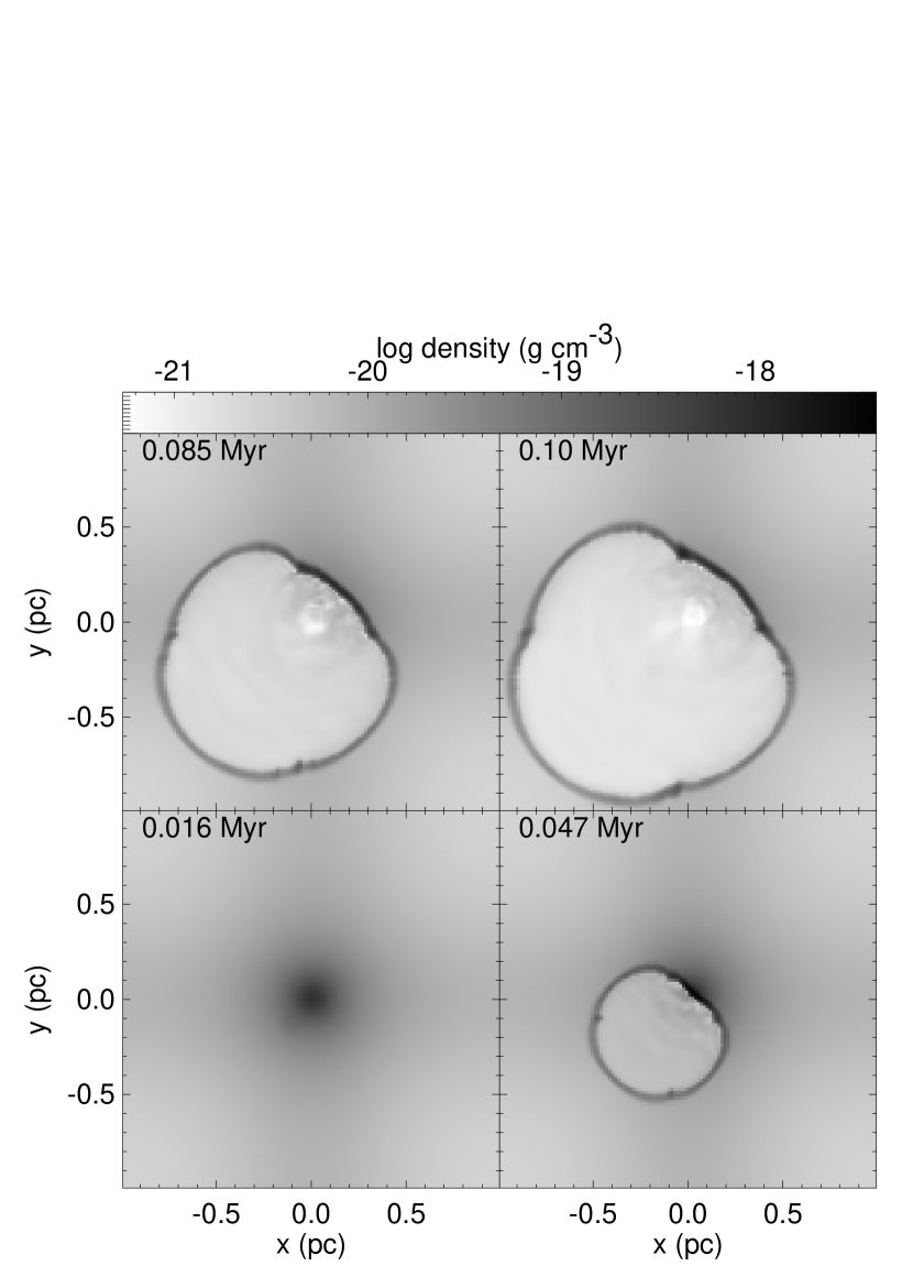
Figure 4: Evolution of H ii region with ionizing source off-center from peak density of a collapsing region formed from initially uniform gas (model D). Times are given in megayears after ionization begins at $t_{ion}$. Shown are two-dimensional cuts through the density field in the $xy$-plane containing the peak density. The source is located behind the cut plane. Greyscale shows log of density, with values given by the colorbar. Artifacts appear directly along grid-lines from the source produced by a slight error in propagating rays in those directions. Note the lack of confinement or cometary morphology in the densest regions.

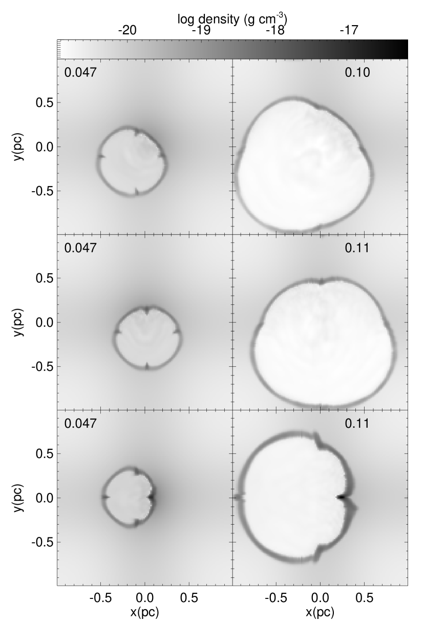
Figure 5: Time evolution of regions with sources at different positions relative to peak density of collapsing region formed from initially uniform gas. Sources are shifted 8 zones (0.125 pc) along the (bottom) $x$-axis, (middle) $y$ and $z$-axes, and (top) $x$, $y$, and $z$-axes, (models B, C, and D, respectively). Cuts along the $xy$ plane in the plane of the source are shown. (The top two panels can be compared to the cuts through the same model in the plane of peak density shown in Figure 4). Times are given in megayears, and the greyscale shows log of density. Artifacts appear directly along grid-lines from the source produced by a slight error in propagating rays in those directions. Morphologies do not depend strongly on position of source.

In Figure 4 we show the time development of the H ii region resulting from turning on an ionizing source 0.22 pc diagonally from the center of the core (model D). As can be seen from Figure 3a, this lies within the power-law envelope. Varying the position of the ionizing source from the inner edge of the envelope at 0.125 pc to the middle of the envelope at 0.22 pc (models B, C, and D) makes little difference to the conclusions drawn here, as shown in Figure 5.

The expansion of the H ii region drives a strong shock into the surrounding gas, sweeping up a thin, dense shell of neutral gas that traps the H ii region for the $10^{5}$ yr duration of these runs. In the smooth core model shown here, the neutral sound speed is 0.2 km s^-1, corresponding to gas with a temperature of order 10 K. Recent work by Franco et al. (2007) uses an effective sound speed more than an order of magnitude higher as an approximation to turbulent motions in order to maintain hydrostatic equilibrium in their cores, rather than following the collapse as we do. As a result they do not see dense shell formation.

Contrary to much early speculation (e.g., Fey et al. 1992; Gaume et al. 1995), the stratification of the spherical envelope produces a nearly spherical H ii region shape during the period that we simulate, rather than a cometary shape. That this might occur was actually first shown in a different context by the analytic work of Korycansky (1992), who used the Kompaneets (1960) approximation to compute the shape of off-center blast waves in spherical, power-law stratified, density distributions. Confinement in conical regions only happens for density power laws steeper than -4. Blast waves expanding into distributions with power laws in the range -4/3 to -8/3 ultimately open out and wrap completely around the central core. Arthur & Hoare (2006) find a similar spherical shape to our own result in their model F, which also includes a stellar wind. This result has been more comprehensively investigated by Arthur (2007) who shows that nearly spherical H ii regions are expected in a wide variety of power-law density distributions, so long as the H ii region does not become unbounded. Franco et al. (2007) found cometary shapes, but it was most likely because they computed two-dimensional models assuming slab symmetry: effectively a line ionizing source near a cylinder. The lack of the possibility of expanding in the third dimension tends to give narrower blowouts (this was also seen by Mac Low, McCray, & Norman 1989 in a different situation).

In the models presented here, the innermost region of the collapsing core is too dense to be ionized. It continues to collapse despite the ionization of its envelope, as shown in Figure 6. Indeed, the impact of the photoionization-driven shell appears if anything to accelerate collapse, as our model B, with the ionizing source closest to the center of the cloud, has a higher peak density over time. However, note that model D, with source somewhat farther from the peak than model C, still ends up with slightly higher density. This may just be the effect of the ray-tracing artifacts which impact the core in model C, and not in model D. A nearby ionizing source will in general have great difficulty preventing collapse in a region that has already reached moderately high density because the recombination rate $\propto n^{2}$ while the ionization rate is only $\propto n$, so as collapse proceeds, more and more photons are required to maintain the ionization of the same region. We discuss this quantitatively below, in § 4.2.

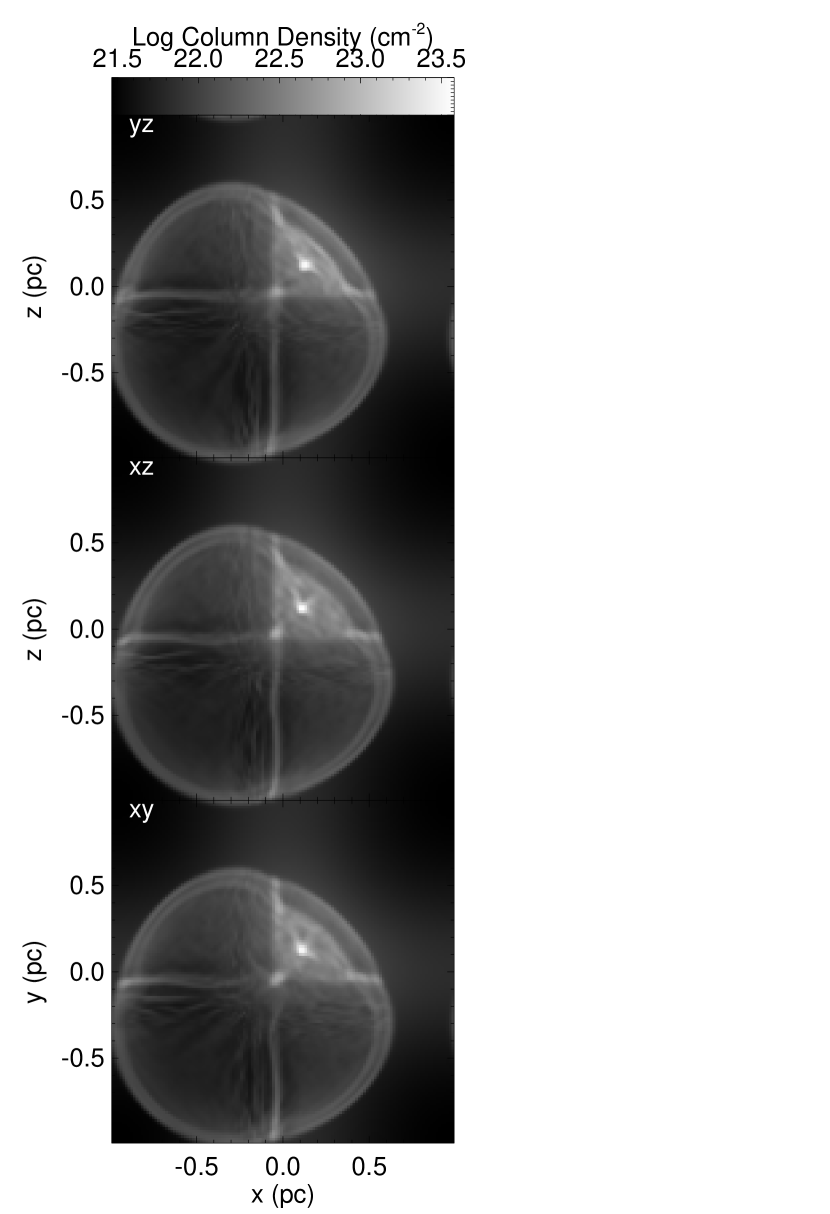
Figure 7: Column density for the sum of neutral and ionized gas (dominated by the neutral gas) in a model of the expansion of an H ii region collapsing from initially uniform gas (model D). Projections are shown along the $x$, $y$, and $z$-axes as indicated, at the same time as the final panel of Figure 4. The bright spot is the center of the dense collapsing core, while the cross-shaped artifact comes from a slight error in propagating rays directly along grid-lines from the source.

Although the shape of the shock front is close to spherical, the intensity of emission from the neutral shell and the ionized interior varies around the shell, as the shell is higher density where it lies nearest to the center of the core (Fig. 4). We do not explicitly show simulated observations of the ionized gas, as artifacts in the boundary layer ionized density, caused by recent ionization of high-density neutral zones, dominate the emission. Instead, we show in Figure 7 the column density $\int nd\ell$, which is dominated by the neutral density.

The highest column density point is at the dense center of the gravitationally collapsing core. Even before this forms a star, as it reaches higher densities and pressures, the gas ionized on its surface also reaches higher densities. This ionized gas may have sufficiently high emission measure to appear as a UCHR, surrounded by a more diffuse compact H ii region, the usual configuration observed (Kim & Koo, 2001). However, it will have a brief lifetime, of order the free-fall time of $10^{4}$ yr or less (see eq. [2]). In the next subsection we consider the development of a more complex flow.

3.2 Turbulent Flow

To understand the development of H ii regions in a more realistic environment, we examine their formation in cores that are self-consistently collapsing from the supersonic turbulent flow characteristic of a molecular cloud. We turn on ionization near the highest density point in the simulation, at the time that the density reaches the Jeans resolution limit. Figure 8 shows that only our highest resolution model remains formally well resolved after collapse begins, but that the behavior of the peak density is reasonably well resolved. To follow the expansion of the H ii region for the longest time possible, we take advantage of the periodic boundary conditions to shift the highest density point to the center of the cube before beginning ionization. Once again, the density structure of the cores takes on a radial density dependence $\rho\propto r^{-2}$ (Fig. 3b).

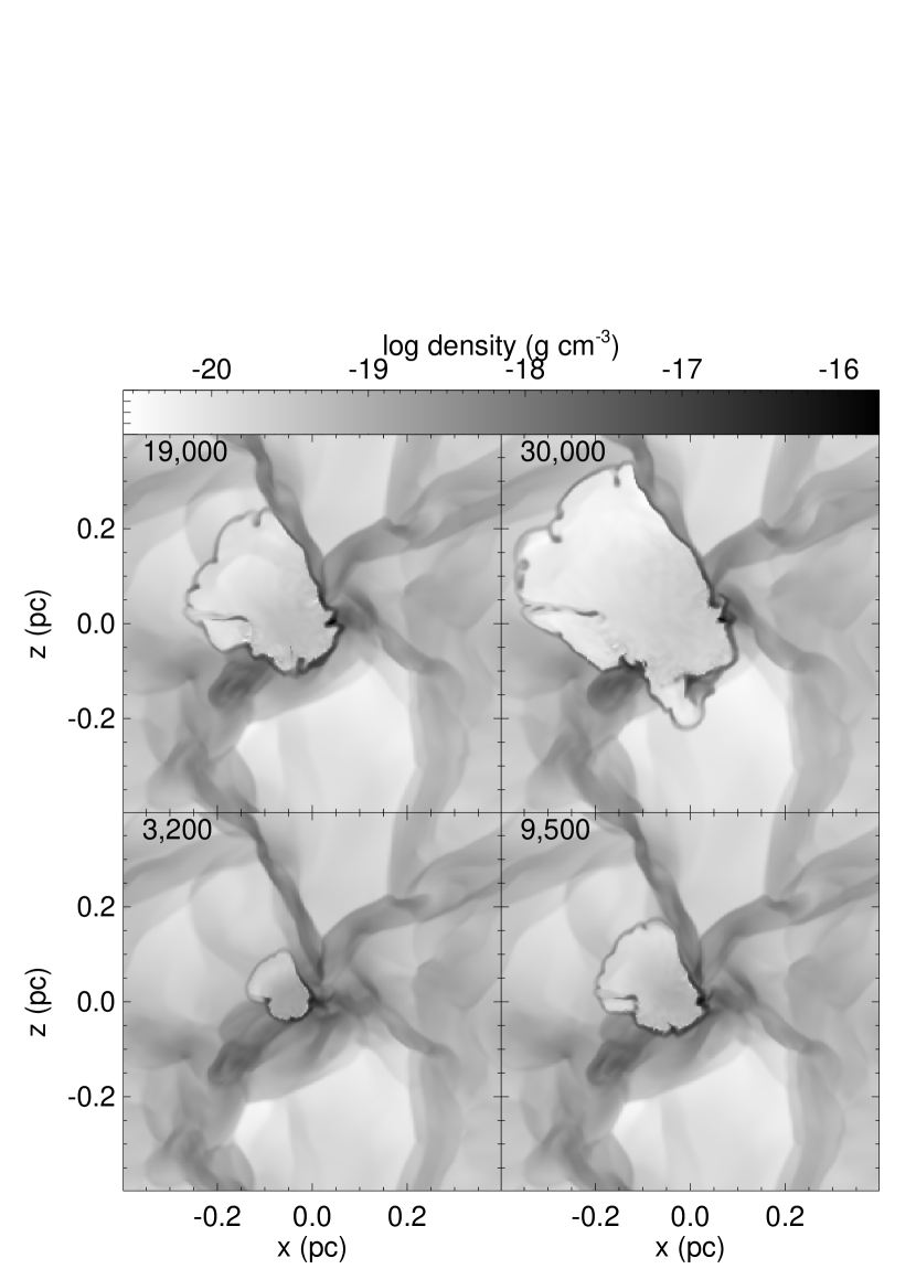
Figure 9: Evolution of H ii region with ionizing source off-center from peak density of a collapsing region formed from initially turbulent gas (model H). Times are given in years after ionization begins at $t_{ion}$. Note change of time units and cube size from Figure 4. Two-dimensional cuts in the $xz$ plane (for comparison with the $xy$ cuts shown in Figure 10) centered on the source, with greyscale showing log of density, are shown.

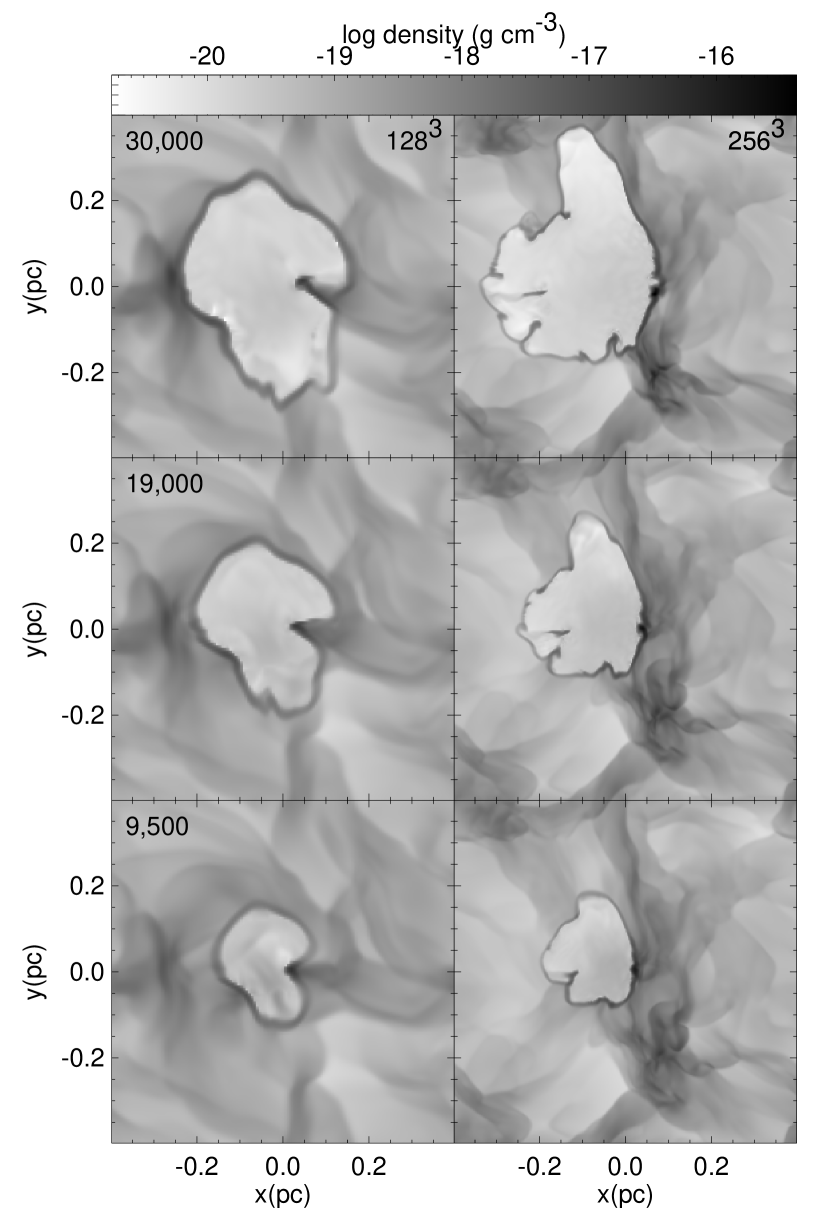
Figure 10: Resolution study of time evolution of region shown in Figure 9, with models E and H shown using $128^{3}$ and $256^{3}$ zones, respectively. Cuts through the $xy$ plane in the plane of the source are shown, for comparison in the $256^{3}$ case to the $xz$ cut shown in Figure 9. The different resolution models use statistically identical turbulence but not the same actual driving pattern, so the shapes should not be compared point by point. Times are again given in years, and the greyscale shows log of density.

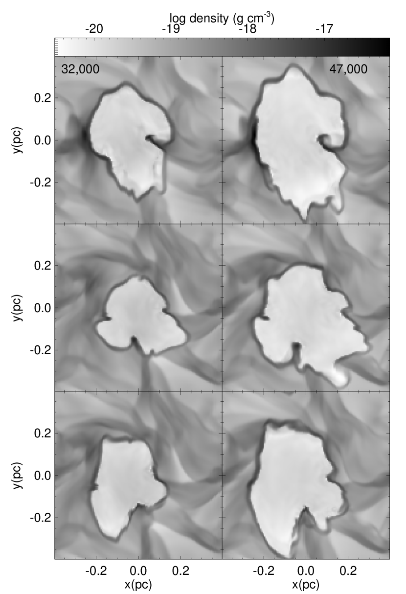
Figure 11: Time evolution of regions with sources at different positions relative to peak density of collapsing region formed from initially turbulent gas. Sources are shifted 8 zones ($0.05$ pc) along the (bottom) $x$-axis, (middle) $y$ and $z$-axes, and (top) $x$, $y$, and $z$-axes (models E, F, and G, respectively). All models use the same turbulent driving pattern, differing only in source position. Cuts through the $xy$ plane in the plane of the source are shown (Note that because of the $z$ shift, this is a different plane in the top panels). Times are given in years, and the greyscale shows log of density.

In Figures 9 and 10 we show the expansion of the resulting H ii region in our highest resolution model H, with the ionizing source only 0.05 pc from the center of the collapsing core, in the inner portion of the power-law envelope. In Figure 10 we compare the morphology of models E ($128^{3}$ zones) and H ($256^{3}$ zones). The primary differences are in the thickness of the shell, which is not fully resolved even at the higher resolution, and in the wavelengths of instability resolved in the shell, again probably not fully resolved. However, the qualitative results that we discuss are ones that the two models agree on. At the lower resolution we varied the position of the ionizing source in models E, F, and G, but, as shown in Figure 11, this again made little qualitative difference. These different models run with the same background density field do give some idea of how sensitive our results are to small perturbations.

The expanding blast wave driven by the ionized gas encounters strong ambient density fluctuations produced by the background supersonic turbulent flow. These fluctuations both directly shape the shell and seed instabilities in the expanding shell. Four instabilities are evident. In regions where the shell is expanding into a sufficiently low density region to begin accelerating, Rayleigh-Taylor instabilities occur. (Strictly speaking, as these are driven by acceleration rather than gravity, they should be denoted Richtmeyer-Meshkov instabilities, as is commonly done in the fluid dynamics community.) Second, a thin, decelerating, pressure-driven, shock-bounded shell is subject to the Vishniac (1983) instability. Our resolution is probably insufficient to capture its saturated state (Mac Low & Norman, 1993), but some clumping seen in the shell will be caused by even an underresolved manifestation of the instability (cf.  Mac Low et al., 1989). Third, the introduction of ionizing radiation impinging on a decelerating shell drives Giuliani (1979) instabilities, as numerically modeled by García-Segura & Franco (1996). Finally, and perhaps most interestingly, the shell itself quickly accumulates enough mass at high enough densities to become gravitationally unstable, something predicted for many years by analytic models (Elmegreen & Lada, 1977; Vishniac, 1983; Voit, 1988).

Although the ionized gas readily expands into low density regions, it does not appear to disrupt the collapsing core. Figure 8 shows no perturbation to the increasing density caused by collapse when ionization turns on at $t=0.83$ Myr. This conclusion is supported by the analytic computation presented below (§ 4.2). The numerical result must be approached with some caution, though, as the Jeans length in the center of the core is resolved by less than four zones during the period after ionization begins.

As gravitational instability in the shell sets in, collapse begins at multiple points. To characterize this behavior, we used the clumpfind algorithm of Williams, de Geus, & Blitz (1994), optimized as described by Klessen, Heitsch, & Mac Low (2000), to find clumps with density at least 10% of the peak density of $5.7\times 10^{-16}$ g cm^-3 in the cube at the last timestep of model H. Contours of 5% of the peak density were used. This captures only regions that are undergoing gravitational collapse, as can be seen from Figure 8, which shows that prior to turning on ionization and gravity, peak densities are approximately 1% of the final peak value. Even accounting for shock compression of those peak densities, we show below in § 4.1 that the peak shell density absent gravitational instability will be only 7% of the peak density.

Aside from the original collapsing core, we find two other collapsing regions with masses of a few solar masses, of the same order of magnitude as the original core. Again, we must emphasize that this is a qualitative result, as these regions have collapsed beyond the Jeans limit. However, they are sufficiently well separated by resolved gas to rule out spurious fragmentation in the shell as causing them. Whether we have fully resolved their internal structure is another matter: we actually found 10 clumps distributed among the three regions, but do not consider this sub-clumping to be well-resolved. We discuss the instability of the shell further in the next section.

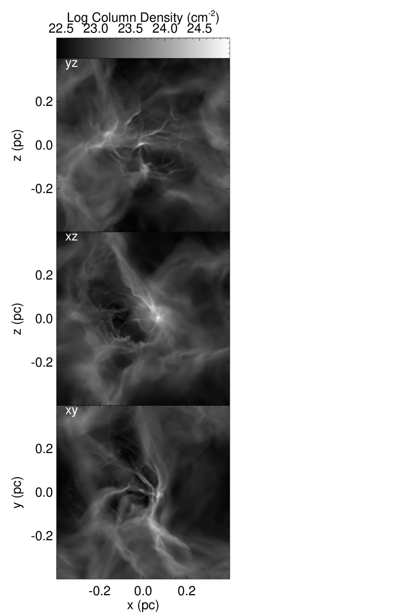
Figure 12: Column density of total gas for a model of the expansion of an H ii region into gas collapsing from initially turbulent state (model H). Projections are shown along the $x$, $y$, and $z$-axes as indicated, at the same time as the final panel of Figure 9.

In Figure 12 we show the column density distribution of the gas in our models. As in Figure 7, this is dominated by neutral molecular gas, while the ionized gas shows up as low column density cavities. There are several points to note about the column density distribution. The material swept up in the neutral shell surrounding the ionized region is distinguishable from the background turbulent gas morphologically. The shell is thinner, with higher contrast and more small-scale structure. This occurs primarily because the background turbulence is at a substantially lower Mach number than the shell, so the structures formed in it are thicker and have lower density contrast. The regions of secondary collapse can also be picked out in the column density projections. In particular, in the $yz$ projection, the regions to the left are clearly separated from the primary core in the center of the image, although they are projected almost on top of each other in the $xz$ projection.

4 Analytic Considerations

4.1 Gravitational Instability

We can understand the observed gravitational collapse by examining the collapse criterion for expanding shells. This was first computed by Elmegreen & Lada (1977) and Elmegreen & Elmegreen (1978), who assumed that turbulent velocities in the shell would be of the same order as the expansion velocity. Ostriker & Cowie (1981) and Vishniac (1983) assumed, on the other hand, that the turbulent velocities in the shell would only be transonic. This latter assumption was supported by analytic work by Voit (1988) and numerical work by Mac Low & Norman (1993). We here use the formulation of this criterion by McCray & Kafatos (1987), who demonstrated that collapse will occur in a spherical shell of radius $R_{s}$, expansion velocity $V_{s}$, ambient density $\rho$, and sound speed $c_{s}$ if the gravitational potential energy in a segment of shell exceeds its pressure and kinetic energy of expansion, a condition that can be expressed as

$$\Upsilon=0.67G\rho R_{s}^{2}/(V_{s}c_{s})\geq 1.$$ (9)

In our case the shell expands into a medium of varying ambient density $\rho$. However, this criterion is derived locally for each patch of shell, so approximating the ambient density with the local value is a reasonable assumption. (Although the ambient density varies radially as well as angularly, most of the mass in any patch of shell accumulates during passage through high density regions near the current radius.)

Our models show shell collapse away from the primary core in the turbulent case, but not in the smooth case. The turbulent model H has a maximum ambient density of $\rho\simeq 5\times 10^{-18}$ g cm^-3 (Fig. 8), a shell radius $R_{s}\simeq 0.25$ pc and velocity $V_{s}\simeq 5$ km s^-1, and sound speed $c_{s}=c_{n}=0.63$ km s^-1, giving $\Upsilon\simeq 4$. Parts of the shell hitting dense filaments in the background turbulent flow become gravitationally unstable and collapse, while parts expanding into lower ambient densities remain stable. The smooth model B, on the other hand, has an average ambient density $\rho\simeq 6\times 10^{-21}$ g cm^-3 with less fluctuation in density from the average than in the turbulent case. Its radius at the end of the run is $R_{s}\simeq 0.5$ pc, and sound speed $c_{n}=0.2$ km s^-1, giving a value of $\Upsilon\simeq 0.06$, in agreement with the lack of collapse found in the model.

The Jeans mass in unstable portions of the shocked shell of model H can be estimated by taking the peak density in the ambient gas, and assuming that it is hit by an isothermal shock of Mach number ${\cal M}=V_{s}/c_{n}\sim 8$, so that the shell density $\rho_{s}={\cal M}^{2}\rho\simeq 4\times 10^{-17}$ g cm^-3, or, in terms of number density, $n_{s}\simeq 10^{7}$ cm^-3. Substituting into equation (1), we find $M_{J}\simeq 2\mbox{ M}_{\odot}$, agreeing within better than 50% with the masses of the observed regions of secondary collapse in model H.

4.2 Trapping Radius

At what radius does an external ionization front get trapped in a collapsing core? We can calculate the initial standoff distance $r_{s}$ of an ionization front impinging on a collapsing core. If $r_{s}$ is small, the core is quickly ionized, while if $r_{s}$ approaches the distance to the ionizing source $d$, the ionization front will have little influence on the core.

The freely collapsing objects formed by gravitational instability in our models have $r^{-2}$ density profiles, while a core with constant central accretion rate $\dot{M}=-4\pi R^{2}\mu n_{0}v_{\rm ff}$, where the free-fall velocity $v_{\rm ff}=-(2GM/R)^{1/2}$, has a shallower $r^{-3/2}$ density profile (e.g. Shu 1992).

We work in the frame of reference of the ionizing source, with distance from the source given by $r$. Along the line connecting the source with the center of the core, $R=d-r$. We take the number density $n(r)=n_{0}(R/R_{0})^{-\eta}$, where $n_{0}$ and $R_{0}$ characterize the mass and size of the core, and $\eta=3/2$ or 2. Assuming the photoionized gas to be fully ionized, ionizing photons are absorbed at a rate

$$\frac{dS}{dr}=-4\pi r^{2}n(r)^{2}\alpha$$ (10)

(e.g. Spitzer 1978), where $\alpha$ is the hydrogen recombination coefficient to the second level. Substituting for density and integrating both sides, we find the stellar ionizing photon luminosity

$$S_{*}=4\pi n_{0}^{2}R_{0}^{2\eta}\alpha\int_{0}^{r_{s}}drr^{2}(d-r)^{-2\eta}.$$ (11)

The integral can be evaluated by substitution of variables for $\eta=3/2$ or 2.

We can place the solutions in dimensionless form. Define the fractional standoff distance of the ionization front from the center of the core along the line of sight to the star $\xi=(d-r_{s})/d$. Small values of $\xi$ mean highly ionized cores, while large values suggest only the core surface is ionized. Then we can define a dimensionless ionizing photon luminosity

$${\cal L}(\eta)=\frac{S_{*}}{4\pi\alpha n_{0}^{2}R_{0}^{2\eta}d^{2\eta-3}}.$$ (12)

Note that for $\eta=3/2$, this dimensionless luminosity is independent of the actual standoff distance of the core $d$. Then, the solution for cores with density power-law $\eta=3/2$ is

$${\cal L}(3/2)=\frac{3}{2}-\ln\xi-\frac{2}{\xi}+\frac{1}{2\xi^{2}},$$ (13)

and for $\eta=2$, it is

$${\cal L}(2)=-\frac{1}{3}+\frac{1}{\xi}-\frac{1}{\xi^{2}}+\frac{1}{3\xi^{3}}.$$ (14)

If we substitute typical values, including ionization coefficient $\alpha=2\times 10^{-13}$ cm³ s^-1, we find

$${\cal L}(3/2)=1.4\left(\frac{S_{*}}{10^{48}\mbox{ s}^{-1}}\right)\left(\frac{n_{0}}{10^{5}\mbox{ cm}^{-3}}\right)^{-2}\left(\frac{R_{0}}{0.01\mbox{ pc}}\right)^{-3},$$ (15)

and

$${\cal L}(2)=(1.4\times 10^{2})\left(\frac{S_{*}}{10^{48}\mbox{ s}^{-1}}\right)\left(\frac{d}{1\mbox{ pc}}\right)\left(\frac{n_{0}}{10^{5}\mbox{ cm}^{-3}}\right)^{-2}\left(\frac{R_{0}}{0.01\mbox{ pc}}\right)^{-4}.$$ (16)

The value of ${\cal L}(\eta)$ determines whether a collapsing core is promptly ionized or remains mostly neutral. The higher value of ${\cal L}(2)$ for the same parameters shows that the corresponding cores are more easily ionized, as expected. In Figure 13 we show the relation between the fractional ionization standoff distance $\xi$ and the dimensionless luminosity ${\cal L}(\eta)$ for $\eta=3/2$ and $2$. For plausible parameters, $\xi$ is sufficiently large to suggest that these cores could form high-emission measure sources for a free-fall time.

We note that observed molecular cloud cores have power-law envelopes with flat interiors (e.g. André, Ward-Thompson, & Barsony 2000). If the calculated stand-off distance for such a core becomes less than the radius of the constant-density central region, we expect the core to be quickly ionized.

4.3 Expected Radio Flux

We can use our knowledge of the trapping radius to make an estimate of the expected radio flux density from the ionized portion of a collapsing core, for comparison with observed UCHRs. We follow Garay (1987), who assume that the flow of ionized gas from a dense core embedded in an H ii region follows an $\eta=2$ power-law density profile. Henney (2003) show analytically that this is likely to be a good approximation for many radial scale lengths away from a core embedded in the wall of an H ii region, while Franco et al. (2000) demonstrate that a number of observed UCHRs have radio spectral indexes consistent with power-law profiles of ionized density.

The radio flux density from an unresolved source depends on whether it is optically thin or thick. Moran (1983) gives the optically thin flux density at frequency $\nu$, using power law opacity (Mezger & Henderson, 1967), as

$$S_{\nu}=(3.4\mbox{ mJy})\left(\frac{\nu}{1\mbox{ GHz}}\right)^{-0.1}\left(\frac{\cal{V}}{10^{57}\mbox{ cm}^{-6}}\right)\left(\frac{T_{e}}{10^{4}\mbox{ K}}\right)^{-0.35}\left(\frac{D}{1\mbox{ kpc}}\right)^{-2},$$ (17)

where $T_{e}$ is the electron temperature, $D$ is the distance, and ${\cal V}=\int n_{e}^{2}dV$ is the volume emission measure, computed from the electron number density $n_{e}$ and the volume of ionized gas $V$. The volume emission measure for an object with ionized number density $n(r)=n_{0}(r/r_{0})^{-2}$ for $r>r_{i}$ can be shown to be ${\cal V}=4\pi n_{0}^{2}r_{i}^{3}$. In our case, the objects in question are density enhancements in the shell. The one-sided nature of the ionization will make about a factor of two difference in the volume emission measure, which we parameterize with a factor $\psi$. Combining this with equation (17), we can write the flux density as (Garay, 1987)

$$S_{\nu}=(5.4\mbox{ mJy})\left(\frac{\psi}{0.5}\right)\left(\frac{n_{i}}{5\times 10^{5}\mbox{ cm}^{-3}}\right)^{2}\left(\frac{r_{i}}{10^{15}\mbox{ cm}}\right)^{3}\left(\frac{\nu}{1\mbox{ GHz}}\right)^{-0.1}\left(\frac{T_{e}}{10^{4}\mbox{ K}}\right)^{-0.35}\left(\frac{D}{1\mbox{ kpc}}\right)^{-2}.$$ (18)

Using equation (16) and Figure 13 we can determine the ionization radius $r_{i}=d(1-\xi)$. We can then find the density at that radius $n_{i}=n_{0}(r_{i}/r_{0})^{-2}$ to derive the flux density expected for any given core parameters, luminosity, and distance.

5 Comparisons to Observations

Our models give insight into the behavior of smaller regions of massive star formation, where many observed UCHRs reside, particularly those picked up in broad surveys such as those of Wood & Churchwell (1989) and Kurtz et al. (1994). These UCHRs are nearly always observed to have associated extended emission (Garay et al., 1993; Kurtz et al., 1999; Kim & Koo, 2001; Bik et al., 2005) consistent with a larger underlying H ii region. Kim & Koo (2001) suggested that this was simply due to the hierarchical structure of molecular clouds, but the lifetimes for the densest regions in their scenario were derived from the photoevaporation timescale (Whitworth, 1979), which can be more than an order of magnitude longer than the Jeans collapse timescale for these dense regions. Instead, the models shown here suggest that the observed UCHRs are short-lived regions of collapse in a longer-lived, larger, expanding shell. Bik et al. (2005) found that many UCHRs do not themselves contain OB stars, but have nearby embedded clusters with OB members. As these clusters have ages of order $10^{6}$ yr, they suggest that the cluster age, rather than the age of individual UCHRs, is the relevant timescale, in agreement with the model presented here.

Unresolved UCHRs in the survey of Wood & Churchwell (1989) have integrated flux densities at 2 and 6 cm in the range of 2–1700 mJy. We can compare the flux density expected for cores in our model to confirm whether it is consistent with the observed range. Unfortunately, the lack of a detailed treatment of the interface between neutral and ionized gas inhibits our ability to directly measure the ionized material flowing off density condensations in the simulated shell as predicted by Henney (2003). Nevertheless, we can make some order of magnitude estimates of the properties of the clumps.

In § 3.2 we showed that regions of secondary collapse typically had masses of a few solar masses, which we’ll take for the example to be $M=2$ M_⊙. To set scales, we choose the background density of the H ii region at the end of model H of $\rho_{0}\simeq 2\times 10^{-20}$ g cm^-3 as the outer edge of the $r^{-2}$ region. Then $r_{0}=(M/4\pi\rho_{0})^{1/3}=0.08$ pc. If we take the mean mass per particle for molecular gas with 10% He nuclei $\mu=3.39\times 10^{-24}$ cm^-3, then $n_{0}=5.9\times 10^{3}$ cm^-3. A typical distance to the central star is $d\simeq 0.2$ pc, and in this model the star’s ionizing luminosity is $S_{*}=10^{49}$ s^-1. Substituting into equation (16), we find ${\cal L}(2)=4\times 10^{-3}$. Examining Figure 13, we find $\xi\simeq 0.86$, and thus $r_{i}=d(1-\xi)=0.028$ pc. The density at that radius is then $n_{i}=n_{0}(r_{i}/r_{0})^{-2}=4.8\times 10^{4}$ cm^-3. We can then use equation (18) to derive the flux density from this object, $S_{\nu}=(970\mbox{ mJy})(D/5\mbox{ kpc})^{-2}(\nu/15\mbox{ GHz})^{-0.1}(T/10^{4}\mbox{ K})^{-0.35}(\psi/0.5)$. For typical values, this is consistent with the flux densities of even bright unresolved objects observed by Wood & Churchwell (1989).

Kurtz et al. (1994) found a direct correlation between size and density of spherical and unresolved UCHRs. They suggested that expanding regions would behave in this way. However, collapse offers an alternative explanation for the observed correlation. Observations of massive star formation regions such as Sag B2 (De Pree et al., 1996, 1998), W3 (Tieftrunk et al., 1997), and W49 (De Pree et al., 1997, 2000) show multiple UCHRs closely spaced. These regions are far larger than the ones simulated here. Further work will need to be done to understand whether these larger regions generate a single expanding shell as here, or many smaller isolated ones. However, collapse in a single expanding shell would again address the lifetime question.

In simple models based on static spherical cores, the calculated number of ionizing photons required for observed UCHRs have typically been found to be factors of 3–10 higher than can be provided by external ionizing sources. However, collapsing structures in a sheet could conceivably produce the same emission measures with fewer photons. This problem requires further investigation.

Most high-resolution observations of H ii regions to date observe either emission from the ionized gas, proportional to the square of the ionized gas density, extinction of the ionized gas by the neutral gas, or near-infrared emission from small dust grains or PAHs, presumably embedded in the neutral gas or the densest ionized gas. The last is determined by a combination of radiative heating from the central star and local dust density. Even sub-millimeter dust emission, which traces column density in cold clouds, will be strongly perturbed by radiative heating near the surface of the H ii region. The pure column density map shown here in Figure 12 is suggestive of the results expected from these different observational methods, but lacking any treatment of radiative heating or direct measure of the ionized density, does not represent a direct simulation of any of them.

That caveat being stated, the shape of the cavity is certainly strongly reminiscent of the observations of larger H ii regions such as those by the GLIMPSE survey with the Spitzer Space Telescope (e.g. Churchwell et al., 2004). In particular, we reproduce the filamentary nature of the dense gas, and the fingerlike protrusions in from the wall of the shell, as well as, naturally, the appearance of an internal cavity. We note that, although we see high column density filaments, the shell is dense in every direction, with the filaments simply being the highest column density regions.

6 Conclusions

We have modeled the dynamical growth of young H ii regions in turbulent, self-gravitating, molecular clouds. Our assumed initial conditions reflect the star formation paradigm reviewed by Mac Low & Klessen (2004). This suggests that massive star formation occurs in cloud cores collapsing from a turbulent flow that are far from hydrostatic equilibrium, as already proposed in the classic review by Shu, Adams, & Lizano (1987). The collapse produces the observed high pressures, so they are transient, lasting only on the order of a free-fall time. The medium from which the collapse occurs has large density fluctuations produced by a supersonic turbulent flow, so that the H ii region resulting from massive star formation expands into an inhomogeneous medium.

Before giving the conclusions we draw from the simulations, we summarize the strengths and limitations of these models. They are fully three-dimensional models including driven, hypersonic turbulence, that use a ray-tracing algorithm to follow direct ionization from a single ionizing star. Although our highest resolution models have $256^{3}$ zones, and resolve the Jeans length with four zones everywhere except the very centers of a few collapsing regions at late times, they do not fully resolve the dense, swept-up shell behind the expanding shock front, nor the denser ionized gas layer coming off of collapsing cores. We use periodic boundary conditions, so large-scale gradients in the molecular gas are not modelled. Scattering of ionizing radiation is not accounted for, so that shadows are sharper than they should be. Magnetic fields are not included in these models, though they might modify the structure of the dense shell. They are unlikely to be strong enough to resist gravitational collapse in the massive star-forming region we are modeling, however. We have artificially extended the heating and cooling timescales, reducing the pressure in the ionized gas at early times, and thus making as much as a 10–20% error in the radii of the resulting H ii regions. Absorption of ionizing radiation by dust is also not included, which can reduce the available ionizing luminosity by an order of magnitude (Petrosian, Silk, & Field, 1972; Arthur et al., 2004), though probably in a uniform fashion that will not impact our qualitative conclusions. Finally, we have not included stellar winds (Arthur & Hoare, 2006), which will drive faster expansion and more accumulation of mass in the swept-up shell, tending to counteract the effect of dust.

Despite their limitations, our models give insight into the nature of UCHRs. We demonstrate that the shape of an H ii region expanding off-center in a core with an $r^{-2}$ power-law density distribution is roughly spherical, confirming the general analytic results of Korycansky (1992). This suggests that simple champagne flow models may have difficulty producing the parabolic shapes characteristic of cometary UCHRs (Wood & Churchwell, 1989). Arthur & Hoare (2006) were able to form the parabolic shapes observed only in a planar density gradient with a stellar wind confining the H ii region. They also find a spherical shape in a spherical core, though (their model F).

The expanding shell of the H ii region takes roughly $10^{5}$ yr to reach a radius of a parsec and break out of its parent molecular cloud. During that time, self-gravitating cores repeatedly collapse in it as it interacts with pre-existing turbulent density fluctuations. While each core collapses in only $\sim 10^{4}$ yr, they form repeatedly over the lifetime of the shell, and can be externally ionized to emit radio fluxes comparable to the observations (§ 4.3). Since these cores will often be too low mass to form OB stars, this scenario might explain both the apparent lifetime of UCHRs of $>10^{5}$ yr (Wood & Churchwell, 1989) and their association with compact H ii regions (Kim & Koo, 2001; Bik et al., 2005).

Work remains to be done to demonstrate the viability of this scenario. Most importantly, the expected velocity structure and detailed emissivity structure for externally ionized cores in an expanding shell need to be computed. The relative importance of externally ionized cores in an expanding shell that might account for unresolved sources, and stars orbiting in a cluster potential that could produce cometary UCHRs also needs further consideration. These two scenarios make distinctly different predictions for the direction of ionized gas flow, and the relationship between ionized and molecular gas.

Table 1: Model Parameters

Model	$L$	nx	IC	G	$S_{48}$	$c_{n}$	$\rho/\rho_{0}$	$N_{J}$	$\Delta x_{src}$	$\Delta y_{src}$	$\Delta z_{src}$
A	2	128	U	N	0.5	0.20	1	$\cdots$	0	0	0
B	2	128	U	Y	10	0.20	3	1390	0.125	0	0
C	2	128	U	Y	10	0.20	3	1390	0	0.125	0.125
D	2	128	U	Y	10	0.20	3	1390	0.125	0.125	0.125
E	0.8	128	T	Y	10	0.63	100	546	0.05	0	0
F	0.8	128	T	Y	10	0.63	100	546	0	0.05	0.05
G	0.8	128	T	Y	10	0.63	100	546	0.05	0.05	0.05
H	0.8	256	T	Y	10	0.63	100	546	0.05	0	0
J	0.8	64	T	Y	10	0.63	100	546	0.05	0	0

Note. — All models have ionized sound speed $c_{i}=10$ km s^-1, and heating and cooling reduction factor $\zeta=10^{-3}$. All turbulent models have driving luminosity $\dot{E}=1.875\times 10^{33}$ erg s^-1 and driving wavelengths $k_{d}=$1–2.

Figure 1: Radius of ionized region in homogeneous medium over time from the theoretical prediction (solid line), and our model A at a resolution of $128^{3}$ zones with values of the heating and cooling reduction factor $\zeta=0.1$ (squares), 0.01 (diamonds), and $10^{-3}$ (asterisks). Computation time linearly increases with $\zeta$ so long as the cooling time step dominates. A model with the same density and temperature as models E–J is also shown crosses, along with its theoretical prediction dashed line.

Figure 2: Central temperature of ionized region in homogeneous medium over time from our model A with values of the heating and cooling reduction factor $\zeta=0.1$ (solid), 0.01 (dotted), and $10^{-3}$ (dashed). The figure shows the slower approach to equilibrium temperature of the lower $\zeta$ model that we use. However, as the thermal timescale depends directly on the density, we also show with the thin dashed line a model with the same density and temperature as models E–J, which approaches equilibrium in far less than a dynamical time. (Note that the dips at late times are caused by the dynamics within the H ii region driven by the rarefaction wave that opens behind the initial shock front.)

Figure 3: Density as a function of radius of the collapsing core immediately before ionization is turned on in (a) a uniform medium along the $x$-axis (128³ model B), and (b) a turbulent medium ($256^{3}$ model H) along the $x$-axis (solid), $y$-axis (dashed), and $z$-axis (dash-dotted). The thin dotted line shows the power law $r^{-2}$ in each case.

Figure 6: Change in peak density over time in models with sources at different positions relative to peak density of collapsing region formed from uniform gas. Sources are shifted 8 zones ($0.125$ pc) along the $x$-axis (solid line), $y$ and $z$-axes (dotted line), and $x$, $y$, and $z$-axes (dashed line). These are models B, C, and D.

Figure 8: Resolution study of maximum density over time for turbulent models with $64^{3}$ (dotted line, model J), $128^{3}$ (dashed line, model E), and $256^{3}$ (solid line, model H) zones. Equilibrium driven turbulence is first allowed to develop, then gravity is turned on at a time shown by the vertical line on the x-axis. The Jeans criterion (Truelove et al., 1997) for the three different resolutions is shown on the outer y-axis.

Figure 13: The dimensionless ionizing luminosity ${\cal L}(\eta)$ required to reach a fractional ionization standoff radius $\xi=(d-r_{s})/d$ for a star a radial distance $r=d$ away from a core with density power-law $n\propto r^{-\eta}$. The core is to the left, the star to the right, so higher luminosity ionizes closer to the center of the core. Solutions are shown for $\eta=3/2$ (dashed) and $\eta=2$ (solid).

References

- Abel & Wandelt (2002) Abel, T., & Wandelt, B. D. 2002, MNRAS, 330, L53
- Abel et al. (1999) Abel, T., Norman, M. L., & Madau, P. 1999, ApJ, 523, 66
- André et al. (2000) André, P. Ward-Thompson, D., & Barsony, M. 2000, in Protostars and Planets IV, eds. V. Mannings, A. P. Boss, & S. S. Russell (Tucson: U. of Arizona Press), 59
- Arons & Max (1975) Arons, J., & Max, C. E. 1975, ApJ, 196, L77
- Arthur (2007) Arthur, S. J. 2007, ApJ, submitted (arxiv:0705.0711)
- Arthur & Hoare (2006) Arthur, S. J., & Hoare, M. G. 2006, ApJS, 165, 283
- Arthur et al. (2004) Arthur, S. J., Kurtz, S. E., Franco, J., & Abarrán, M. Y. 2004, ApJ, 608, 282
- Benjamin et al. (2001) Benjamin, R. A., Benson, B. A., & Cox, D. P. 2001, ApJ, 554, L225
- Bik et al. (2005) Bik, A., Kaper, L., Hanson, M. M., & Smits, M. 2005, A&A, 440, 121
- Bodenheimer et al. (1979) Bodenheimer, P., Tenorio-Tagle, G., & Yorke, H. W. 1979, ApJ, 233, 85
- Burkert & Bodenheimer (1993) Burkert, A., & Bodenheimer, P. 1993, MNRAS, 264, 798
- Bonnell et al. (1997) Bonnell, I. A., Bate, M. R., Clarke, C. J., & Pringle, J. E. 1997, MNRAS, 285, 201
- Bonnell et al. (2004) Bonnell, I. A., Vine, S. G., & Bate, M. R. 2004, MNRAS, 349, 734
- Churchwell (1999) Churchwell, E. 1999, in The Origin of Stars and Planetary Systems, eds. C. J. Lada & N. D. Kylafis, (Dordrecht: Reidel) 515
- Churchwell (2002) Churchwell, E. 2002, ARA&A, 40, 27
- Churchwell et al. (2004) Churchwell, E. et al. 2004, ApJS, 154, 322
- Comerón & Torra (1996) Comerón, F., & Torra, J. 1996, A&A, 314, 776
- Dale et al. (2005) Dale, J. E., Bonnell, I. A., Clarke, C. J., & Bate, M. R. 2005, MNRAS, 358, 291
- Dalgarno & McCray (1972) Dalgarno, A., & McCray, R. A. 1972, ARA&A, 10, 375
- De Pree et al. (1995) De Pree, C. G., Rodríguez, L. F., & Goss, W. M. 1995, Rev. Mex. Astron. Astrof., 31, 39
- De Pree et al. (1996) De Pree, C. G., Gaume, R. A., Goss, W. M., & Claussen, M. J. 1996, ApJ, 464, 788
- De Pree et al. (1998) De Pree, C. G., Goss, W. M., & Gaume, R. A. 1998, ApJ, 500, 847
- De Pree et al. (1997) De Pree, C. G., Mehringer, D. M., & Goss, W. M. 1997, ApJ, 482, 307
- De Pree et al. (2000) De Pree, C. G., Wilner, D. J., Goss, W. M., Welch, W. J., & McGrath, E. 2000, ApJ, 540, 308
- Dyson et al. (1995) Dyson, J. E., Williams, R. J. R., & Redman, M. P. 1995, MNRAS, 277, 700
- Elmegreen & Elmegreen (1978) Elmegreen, B. G., & Elmegreen, D. M. 1978, ApJ, 220, 1051
- Elmegreen & Lada (1977) Elmegreen, B. G., & Lada, C. 1977, ApJ, 214, 725
- Falgarone et al. (1992) Falgarone, E., Puget, J.-L., & Perault, M. 1992, A&A, 257, 715
- Fey et al. (1992) Fey, A. L., Claussen, M. J., Gaume, R. A., Nedoluha, G. E., & Johnston, K. J. 1992, AJ, 103, 234
- Franco et al. (1990) Franco, J., Tenorio-Tagle, G., & Bodenheimer, P. 1990, ApJ, 349, 126
- Franco et al. (2007) Franco, J., García-Segura, G., Kurtz, S. 2007. ApJ, 660, 1296
- Franco et al. (2000) Franco, J., Kurtz, S., Hofner, P., Testi, L., García-Segura, G., & Martos, M. 2000, ApJ, 542, L143
- Frigo & Johnson (2005) Frigo, M., & Johnson, S. G. 2005, Proc. IEEE, 93, 216
- Fryxell et al. (2000) Fryxell, B. et al. 2000, ApJS, 131, 273
- Garay (1987) Garay, G. 1987, Rev. Mex. Astron. Astrof., 14, 489
- Garay et al. (1993) Garay, G., Rodriguez, L. F., Moran, J. M., & Churchwell, E. 1993, ApJ, 418, 368
- García-Segura & Franco (1996) García-Segura, G., & Franco, J. 1996, ApJ, 469, 171
- Gaume et al. (1995) Gaume, R. A., Claussen, M. J., De Pree, C. G., Goss, W. M., & Mehringer, D. M. 1995, ApJ, 449, 663
- Giuliani (1979) Giuliani, J. L., Jr. 1979, ApJ, 233, 280
- Glover & Mac Low (2007) Glover, S. C. O., & Mac Low, M.-M. 2007, ApJS, 169, 239
- Henney (2003) Henney, W. J. 2003, Rev. Mex. Astron. Astrof., Ser. Conf., 15, 175
- Hollenbach et al. (1994) Hollenbach, D., Johnstone, D., Lizano, S., & Shu, F. 1994, ApJ, 428, 654
- Humphreys & McElroy (1984) Humphreys, R. M., & McElroy, D. B. 1984, ApJ, 284, 565
- Jeans (1902) Jeans J. H. 1902, Phil. Trans. Roy. Soc., 199, 1
- Kahn (1954) Kahn, F. D. 1954, Bull. Astron. Inst. Netherlands, 12, 187
- Kim & Koo (2001) Kim, K.-T., & Koo, B.-C. 2001, ApJ, 549, 979
- Klessen et al. (2000) Klessen, R. S., Heitsch, F., & Mac Low, M.-M. 2000, ApJ
- Kompaneets (1960) Kompaneets, A. S. 1960, Dokl. Akad. Nauk SSSR, 130, 1001 [Sov. Phys. Dokl., 5, 46]
- Korycansky (1992) Korycansky, D. G. 1992, ApJ, 398, 184
- Krumholz et al. (2006) Krumholz, M. R., Stone, J. M., & Gardiner, T. A. 2006, ApJ, submitted (astro-ph/0606539)
- Kurtz et al. (1994) Kurtz, S. E., Churchwell, E., & Wood, D. O. S. 1994, ApJS, 91, 659
- Kurtz et al. (1999) Kurtz, S. E., Watson, A. M., Hofner, P., & Otte, B. 1999, ApJ, 514, 232
- Larson (1982) Larson, R. B. 1982, MNRAS, 200, 159
- Li et al. (2004) Li, Y., Mac Low, M. -M., & Abel, T. 2004, ApJ, 610, 339
- Lizano et al. (1996) Lizano, S., Canto, J., Garay, G, & Hollenbach, D. 1996, ApJ, 469, 739
- Mac Low (1999) Mac Low, M.-M. 1999, ApJ, 524, 169
- Mac Low & Klessen (2004) Mac Low, M.-M., & Klessen, R. S. 2004, Rev. Mod. Phys., 76, 125
- Mac Low et al. (1989) Mac Low, M.-M., McCray, R., & Norman, M. L. 1989, ApJ, 337, 141
- Mac Low & Norman (1993) Mac Low, M.-M., & Norman, M. L. 1993, ApJ, 407, 207
- Mac Low et al. (1991) Mac Low, M.-M., Van Buren, D., Wood, D. O. S., & Churchwell, E. 1991, ApJ, 369, 395
- Matzner (2002) Matzner, C. D., 2002, ApJ, 566, 302
- McCray & Kafatos (1987) McCray, R., & Kafatos, M. 1987, ApJ, 317, 190
- Mellema et al. (2006) Mellema, G., Arthur, S. J., Henney, W. J., Iliev, I. T., & Shapiro, P. R. 2006, ApJ, 647, 397
- Mezger & Henderson (1967) Mezger, P. G., & Henderson, A. P. 1967, ApJ, 147, 417
- Moran (1983) Moran, J. M. 1983, Rev. Mex. Astron. Astrof., 7, 95
- Norman (2000) Norman, M. L. 2000, Rev. Mex. Astron. Astrofis., 9, 66
- Ostriker & Cowie (1981) Ostriker, J. P., & Cowie, L. 1981, ApJ, 243, L127
- Petrosian et al. (1972) Petrosian, V., Silk, J., & Field, G. F. 1972, ApJ, 177, L69
- Press et al. (1992) Press, W. H., Flannery, B. P., Teukolsky, S. A., & Vetterling, W. T. 1992, Numerical Recipes in fortran 77 (Cambridge: Cambridge U. Press)
- Raymond et al. (1976) Raymond, J. C., Cox, D. P., & Smith, B. W. 1976, ApJ, 204, 290
- Redman et al. (1996) Redman, M. P., Williams, R. J. R., & Dyson, J. E. 1996, MNRAS, 280, 661
- Redman et al. (1998) Redman, M. P., Williams, R. J. R., & Dyson, J. E. 1998, MNRAS, 298, 33
- Sarazin (1986) Sarazin, C. L. 1986, Rev. Mod. Phys. 58, 1
- Scalo (1986) Scalo, J. M. 1986, Fund. Cosmic Phys., 11, 1
- Sandford et al. (1982) Sandford, M. T., Whitaker, R. W., & Klein, R. I. 1982, ApJ, 260, 183
- Sandford et al. (1984) Sandford, M. T., Whitaker, R. W., & Klein, R. I. 1984, ApJ, 282, 178
- Spitzer (1978) Spitzer, L., Jr. 1978, Physical Processes in the Interstellar Medium (New York: John Wiley & Sons), 109
- Shu (1992) Shu, F. H. The Physics of Astrophysics, Vol. II. Gas Dynamics (Mill Valley, CA: University Science Books), 245
- Shu et al. (1987) Shu, F. H., Adams, F. C., & Lizano, S., ARA&A, 25, 23
- Stone & Norman (1992) Stone, J. M., & Norman, M. L. 1992, ApJS, 80, 753
- Stone et al. (1998) Stone, J. M., Ostriker, E. C., & Gammie, C. F. 1998, ApJ, 508, L99
- Tenorio-Tagle (1979) Tenorio-Tagle, G. 1979, A&A, 71, 59
- Tenorio-Tagle (1982) Tenorio-Tagle, G. 1982, in Regions of Recent Star Formation, eds. R. S. Roger, & P. E. Dewdney (Dordrecht: Reidel), 1
- Tieftrunk et al. (1997) Tieftrunk, A. R., Gaume, R. A., Claussen, M. J., Wilson, T. L., & Johnston, K. J. 1997, A&A, 318, 931
- Truelove et al. (1997) Truelove, J. K., Klein, R. I., McKee, C. F., Holliman, J. H., II, Howell, L. H., & Greenough, J. A., 1997, ApJ, 489, L179
- Van Buren et al. (1990) Van Buren, D., Mac Low, M.-M., Wood, D. O. S., & Churchwell, E. 1990, ApJ, 353, 570
- Van Leer (1977) Van Leer, B. 1977, J. Comput. Phys., 23, 276
- Vishniac (1983) Vishniac, E. T. 1983, ApJ, 274, 152
- Voit (1988) Voit, G. M. 1988, ApJ, 331, 343
- Whitworth (1979) Whitworth, A. 1979, MNRAS, 186, 59
- Williams et al. (1994) Williams, J. P., de Geus, E. J., & Blitz, L. 1994, ApJ, 428, 693
- Williams et al. (1996) Williams, R. J. R., Dyson, J. E., & Redman, M. P. 1996, MNRAS, 280, 667
- Williams & McKee (1997) Williams, J. P., & McKee, C. F. 1997, ApJ, 476, 166
- Wood & Churchwell (1989) Wood, D. O. S., & Churchwell, E. 1989, ApJS, 69, 831
- Xie et al. (1996) Xie, T., Mundy, L. G., Vogel, S. N., & Hofner, P. 1996, ApJ, 473, L131.
- Yorke et al. (1982) Yorke, H. W., Bodenheimer, P., & Tenorio-Tagle, G. 1982, A&A, 108, 25
- Yorke (1986) Yorke, H. W. 1986, ARA&A, 24, 49
- Zinnecker (1982) Zinnecker, H. 1982, Ann. New York Acad. Sci., 395, 226