Density profiles of galaxy groups and clusters from SDSS galaxy-galaxy weak lensing

Abstract

We present results of a measurement of the shape of the density profile of galaxy groups and clusters traced by 43 335 Luminous Red Galaxies (LRGs) with spectroscopic redshifts from the Sloan Digital Sky Survey (SDSS). The galaxies are selected such that they are the brightest within a cylindrical aperture, split into two luminosity samples, and modeled as the sum of stellar and dark matter components. We present a detailed investigation of many possible systematic effects that could contaminate our signal and develop methods to remove them, including a detected intrinsic alignment for galaxies within 100$h^{-1}$kpc of LRGs which we remove using photometric redshift information. The resulting lensing signal is consistent with NFW profile dark matter halos; the SIS profile is ruled out at the 96 (conservatively) and 99.96 per cent confidence level (CL) for the fainter and brighter lens samples (respectively) when we fit using lensing data between 40 $h^{-1}$kpc and $2$ $h^{-1}$Mpc with total signal-to-noise of $19$ and $25$ for the two lens samples. The lensing signal amplitude suggests that the faint and bright sample galaxies typically reside in haloes of mass $(2.9\pm 0.4)\times 10^{13}h^{-1}M_{\odot}$ and $(6.7\pm 0.8)\times 10^{13}h^{-1}M_{\odot}$ respectively, in good agreement with predictions based on halo spatial density with normalization lower than the ’concordance’ $\sigma_{8}=0.9$. When fitting for the concentration parameter in the NFW profile, we find $c=5.0\pm 0.6({\rm stat})\pm 1({\rm sys})$, and $c=5.6\pm 0.6({\rm stat})\pm 1({\rm sys})$ for the faint and bright samples, consistent with $\Lambda$CDM simulations. We also split the bright sample further to determine masses and concentrations for cluster-mass halos, finding mass $(1.3\pm 0.2)\times 10^{14}h^{-1}M_{\odot}$ for the sample of LRGs brighter than $-22.6$ in r. We establish that on average there is a correlation between the halo mass and central galaxy luminosity relation that scales as $M\propto L^{2}$.

1 Introduction

Elliptical galaxies, particularly Luminous Red Galaxies (LRGs), are good tracers of the most massive galactic halos. They have a number of useful properties, including simple, well-understood spectral energy distributions that can be modeled as a passively-evolving burst of star formation, with a constant low level of ongoing star formation; variation with environment that is quantified as well (Eisenstein et al., 2001; Bruzual & Charlot, 2003; Eisenstein et al., 2003); uniform photometric properties, including the fundamental plane relating luminosity, radius, and central velocity dispersion (Faber, 1973; Visvanathan & Sandage, 1977; Djorgovski & Davis, 1987; Kormendy & Djorgovski, 1989; Bower et al., 1992; Roberts & Haynes, 1994; Bernardi et al., 2003) of which the Faber-Jackson relation (Faber & Jackson, 1976) is a projection; and simple light profiles, the de Vaucouleurs profile, with $I\propto\exp(-r^{1/4})$. Galaxies on the massive end of the red sequence contain the majority of the stellar mass of the universe (Fukugita et al., 1998; Hogg et al., 2002; Bell et al., 2004; Baldry et al., 2004; Cool et al., 2006), and hence their properties are of great interest. It was shown that while elliptical galaxies dominate over spirals in overdense environments, these galaxies do reside in a wide variety of environments, from the field to the richest clusters (Morgan et al. 1975; Albert et al. 1977; Ponman et al. 1994; Vikhlinin et al. 1999; Loh & Strauss, 2006, in prep.), with the majority of the LRGs located in group to small cluster sized halos. There have also been extensive studies of LRG clustering (Eisenstein et al., 2005a; Eisenstein et al., 2005b; Masjedi et al., 2005; Zehavi et al., 2005) from 10 $h^{-1}$kpc to 100 $h^{-1}$Mpc scales.

In addition to the extensive photometric studies of elliptical galaxies already in the literature, we would like to add a good understanding of their density profiles. This information is useful for several purposes. First, the dark matter profile can give us information that can be related to the formation history and merger history of these galaxies. Second, the shape of dark matter (DM) profiles can be predicted using N-body simulations (Navarro et al., 1996; Fukushige & Makino, 1997; Kravtsov et al., 1997; Moore et al., 1998; Avila-Reese et al., 1999; Ghigna et al., 2000; Jing & Suto, 2000; Bullock et al., 2001; Klypin et al., 2001; Fukushige & Makino, 2001; Wechsler et al., 2002; Fukushige & Makino, 2003; Zhao et al., 2003; Tasitsiomi et al., 2004; Diemand et al., 2005), though with some disagreement in the value of inner asymptotic logarithmic slope, possibly due to resolution issues, and hence LRGs in massive halos provide a particularly good way of testing the density profile predictions of $\Lambda$CDM. The brightest red galaxies have been shown to have small baryon fractions compared to fainter red galaxies and compared to typical blue galaxies (Mandelbaum et al. 2005d), so the effects of baryons on the DM profile are relatively small in this class of galaxies. Furthermore, since the virial radii are so large, and the concentration parameters decrease with mass, any changes in logarithmic slope around the scale radius occur at large scales relative to smaller galaxies, and hence are easier to measure using the tools available.

While the matter distributions in elliptical galaxies can be simply probed on small scales (within a few $r_{e}$) using central velocity dispersions (Kronawitter et al., 2000; de Zeeuw et al., 2002; Padmanabhan et al., 2004), finding probes of the dark matter profiles on larger scales is more challenging. Kinematic tracers such as satellite galaxies can give information out to tens of $h^{-1}$kpc. Hydrostatic analyses of X-ray intensity profiles, and strong- and weak-lensing constraints for individual clusters, are numerous but thus far do not give a single clear picture (Allen, 1998; Clowe et al., 2000; Clowe & Schneider, 2001; Rusin & Ma, 2001; Sheldon et al., 2001; Athreya et al., 2002; Arabadjis et al., 2002; Koopmans & Treu, 2003; Huterer & Ma, 2004; Ferreras et al., 2005; Vikhlinin et al., 2005; Fukazawa et al., 2006; Humphrey et al., 2006; Koopmans et al., 2006). Weak lensing is another tool that can be used out to scales of several $h^{-1}$Mpc, and the SDSS provides a particularly advantageous dataset due to its significant sky coverage and spectroscopic redshifts (which allow us to determine the profile as a function of transverse separation). Hoekstra et al. (2001) and Parker et al. (2005) have done a group lensing analysis with a much smaller sample ($\sim 100$) groups from CNOC2; however, these small samples are not sufficient to allow a detailed determination of the shape of the density profile.

Measurements of the 3-dimensional density profiles can be used to learn about cosmology as well. For example, the concentration parameter of the profile can be related to the halo mass via the dark matter power spectrum normalization $\sigma_{8}$ and the matter density $\Omega_{m}$. Thus, measuring the profile for several samples of varying halo mass can teach us about the underlying cosmology.

We begin in §2 with a description of the theory behind the measurement we are making. §3 has a full description of the dataset used, including the properties of the lens and source samples, and possible causes of systematic error. We present results of profile measurements in §4, and conclude in §5.

Here we note the cosmological model and units used in this paper. All computations assume a flat $\Lambda$CDM universe with $\Omega_{m}=0.3$, $\Omega_{\Lambda}=0.7$, and $\sigma_{8}=0.9$. Distances quoted for transverse lens-source separation are comoving (rather than physical) $h^{-1}$kpc, where $H_{0}=100\,h$ km$\mathrm{s}^{-1}\,\mathrm{Mpc}^{-1}$. Likewise, $\Delta\Sigma$ is computed using the expression for $\Sigma_{c}^{-1}$ in comoving coordinates, Eq. 4. In the units used, $H_{0}$ scales out of everything, so our results are independent of this quantity. Finally, 2-dimensional separations are indicated with the capital $R$, 3-dimensional radii with lower-case $r$ (occasionally $r$ may denote $r$-band magnitude as well).

2 Theory

Here we describe the theory behind our attempts to measure the three-dimensional density profile using the galaxy-galaxy weak lensing signal.

2.1 Lensing

Galaxy-galaxy weak lensing provides a simple way to probe the connection between galaxies and matter via their cross-correlation function

$$\xi_{g,m}(\vec{r})=\langle\delta_{g}(\vec{x})\delta_{m}^{*}(\vec{x}+\vec{r})\rangle$$ (1)

where $\delta_{g}$ and $\delta_{m}$ are overdensities of galaxies and matter, respectively. This cross-correlation can be related to the projected surface density

$$\Sigma(R)=\overline{\rho}\int\left[1+\xi_{g,m}\left(\sqrt{R^{2}+\chi^{2}}\right)\right]d\chi$$ (2)

(where $r^{2}=R^{2}+\chi^{2}$) which is then related to the observable quantity for lensing,

$$\Delta\Sigma(R)=\gamma_{t}(R)\Sigma_{c}=\overline{\Sigma}(<R)-\Sigma(R),$$ (3)

where the second relation is true only in the weak lensing limit, for a matter distribution that is axisymmetric along the line of sight (which is naturally achieved by our procedure of stacking thousands of lenses to determine their average lensing signal). This observable quantity can be expressed as the product of two factors, a tangential shear $\gamma_{t}$ and a geometric factor

$$\Sigma_{c}=\frac{c^{2}}{4\pi G}\frac{D_{S}}{D_{L}D_{LS}(1+z_{L})^{2}}$$ (4)

where $D_{L}$ and $D_{S}$ are angular diameter distances to the lens and source, $D_{LS}$ is the angular diameter distance between the lens and source, and the factor of $(1+z_{L})^{-2}$ arises due to our use of comoving coordinates. For a given lens redshift, $\Sigma_{c}^{-1}$ rises from zero at $z_{s}=z_{L}$ to an asymptotic value at $z_{s}\gg z_{L}$; that asymptotic value is an increasing function of lens redshift.

For this paper, we are primarily interested in the contribution to the galaxy-mass cross-correlation from the galaxy halo profile itself (central galaxy Poisson term), rather than from neighboring halos (halo-halo term), and hence

$$\Sigma(R)=\int_{-\infty}^{\infty}\rho(r=\sqrt{\chi^{2}+R^{2}})d\chi$$ (5)

The halo-halo term for galaxies in host halos can be modeled simply using the galaxy-dark matter cross-power spectrum as in, e.g., Mandelbaum et al. (2005b), and is only important for $R>2$ $h^{-1}$Mpc, which is the maximum scale probed in this paper.

2.2 Profiles

In previous analyses (Mandelbaum et al., 2005b, d), we have modeled the lensing signal as the sum of contributions from central galaxies (those that lie in host halos) and from satellite galaxies (those that lie in subhalos). For this work, to simplify interpretation by avoiding issues such as tidal stripping of satellites and the radial distribution of satellites within host halos, we use methods (described in §3.1) that enable us to isolate a sample of central galaxies with negligible contamination from satellites. Thus, for this work, our interpretation is much simpler, and can be related directly to $\rho(r)$ for the lens sample under consideration.

While more complicated models may be useful for techniques capable of resolving smaller scale information than this work (minimum transverse separation of 20 $h^{-1}$kpc), we model each galaxy as the sum of two components. The first component is a dark matter profile, with the following density profile:

$$\rho(r)=\frac{\rho_{s}}{\left(r/r_{s}\right)^{-\alpha}\left(1+r/r_{s}\right)^{\alpha+\beta}}.$$ (6)

which gives a logarithmic slope of

$$\frac{{\rm d}\ln{\rho}}{{\rm d}\ln{r}}=\alpha-(\alpha+\beta)\frac{r/r_{s}}{1+r/r_{s}},$$ (7)

or $\alpha$ for $r\ll r_{s}$ and $-\beta$ for $r\gg r_{s}$. This profile with $\alpha=-1$ and $\beta=3$ is the NFW profile (Navarro et al., 1996), and this shape (with varying values of $\alpha$) is a generic prediction of $\Lambda$CDM N-body simulations over a large range of masses. In addition to the logarithmic slopes, it can be defined by two parameters, $c=r_{vir}/r_{s}$ and $M$. The virial radius $r_{vir}$ and $\rho_{s}$ can be related to $M$ via consistency relations. The first is that the virial radius is that within which the average density is equal to $180\overline{\rho}$:

$$M=\frac{4\pi}{3}r_{vir}^{3}\left(180\overline{\rho}\right)$$ (8)

Note that this definition differs from the oft-used $200\rho_{crit}$ definition of mass by roughly 30 per cent for typical values of concentration. The second relation, used to determine $\rho_{s}$ from $M$ and $c$, is simply that the volume integral of the density profile out to the virial radius must equal the virial mass (though when computing the signal, we do not truncate the profiles beyond $r_{vir}$). In principle, the NFW $c$ is a weakly decreasing function of halo mass, with a variety of expressions used (Bullock et al., 2001; Eke et al., 2001), making this profile a one-parameter family of profiles, but in order to give generality to the fits, we allow it to be a free parameter.

To generate the profile at a particular redshift, we start with a given mass, use Eq. 8 to get the comoving virial radius using the comoving matter density, so that $M$, $\alpha$, $\beta$, and $c$ define the profile uniquely. When computing the lensing signal, we are actually averaging over a range of redshifts, which means that since we define the profile in comoving coordinates, we expect that the measured profile will be somewhat blurred due to evolution of concentration with redshift.

While the more general ellipsoidal versions of these density profiles are seen universally in $\Lambda$CDM simulations, here we work only with the spherical versions, because our process of averaging over thousands of lens galaxies makes the results insensitive to halo triaxiality. This statement is not made on the basis of analytical proofs (and surely must be wrong if one requires an extremely high level of precision), but rather on the basis of the lensing signal measured in N-body simulations as an average over randomly-oriented triaxial NFW profiles. In Mandelbaum et al. (2005b), it was shown that spherical NFW profiles do an excellent job at describing the lensing signal for a variety of luminosity bins, with the masses and concentrations of the best-fit profiles related to the real masses and concentrations in the simulations in a particular way (to be discussed further below). The fit $\chi^{2}$ values were very good when the errorbars used on the signal were one-tenth of our current errorbars, so henceforth we consider only spherical NFW fits rather than trying to account for the averaging of triaxial halos.

The second component to the full $\rho(r)$ that we consider is the baryon density. This includes not only the stellar mass, but also any baryons that did not form stars. Read & Trentham (2005) estimate that 80 per cent of the baryonic mass in galaxies is in the form of stars, though for elliptical galaxies this number is closer to 100 per cent, so there is very little gas that has not been converted to stars. As is commonly done for ellipticals, we model the $\rho(r)$ for the stellar component as a Hernquist profile since it is a deprojected de Vaucouleurs profile. The Hernquist profile can be expressed via Eq. 6 with $\alpha=-1$ and $\beta=4$ (and hence falls off faster than an NFW profile on large scales). In the absence of further information about any “dark” baryonic component, we do not model its profile separately, with the expectation that the need for a dark baryonic component will be shown by poor fits in the inner regions.

Finally, we cannot in reality assume that these density profiles are independent. The gravitational potential due to one will necessarily affect the form of the other, so the dark matter profile will not be expected to conform exactly to the ones seen in N-body simulations on small scales where baryonic matter is significant. This effect is known as adiabatic contraction (AC, Blumenthal et al. 1986, Gnedin et al. 2004, Gnedin 2005, Sellwood & McGaugh 2005) and has been studied with analytic models and simulations. To model adiabatic contraction, we use the contra code from Gnedin (2005) to obtain adiabatically-contracted density profiles $\rho(r)$. Generally, on the scales we consider, which are several times the de Vaucouleurs radius, we will show that AC leads to an immeasurably small change in the profile, and hence is not necessary for this work. This is because of low baryonic fractions in these galaxies.

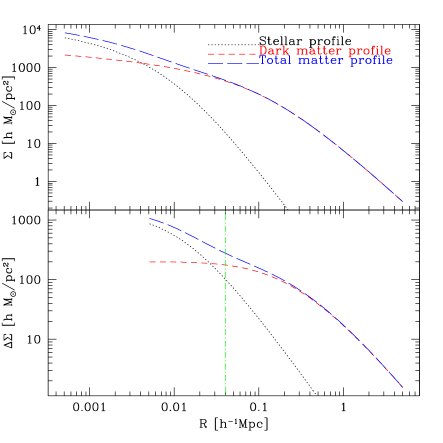
Figure 1 shows the density profile $\rho(r)$ for a typical expected LRG profile, with $M_{NFW}=6\times 10^{13}h^{-1}M_{\odot}$, $M_{b}=8\times 10^{11}h^{-1}M_{\odot}$, $c=7$, baryonic $r_{s}=10$ $h^{-1}$kpc, $\alpha=-1$, $\beta=3$, $\Sigma_{c}^{-1}=2h^{-1}\times 10^{-4}pc^{2}M_{\odot}^{-1}$, with and without AC. The source for these numbers are the predicted LRG masses from the halo mass function, a calculation that will be described shortly.

Figure 1: Density profile $\rho(r)$ for the typical LRG described in the text, including the profile separately for dark matter and for baryons, the total profile, and the total profile including AC (barely distinguishable from the profile without AC), as labelled on the plot.

Given that we measure the lensing signal for projected separations $R>20$ $h^{-1}$kpc, and fit using $R>40$ $h^{-1}$kpc, one might wonder why a baryonic component is necessary for our modeling at all, given the values of the density profiles in Fig. 1 at these separations. We present Fig. 2 to answer this question. The top panel of this figure shows the projected surface density $\Sigma$ as a function of transverse separation for the same density profile as in Fig. 1, and the bottom panel shows the surface density contrast, $\Delta\Sigma$, which is the quantity of interest for lensing. As shown in the top panel of Fig. 2, the baryonic component produces a significant increase in the surface density for transverse separations $R<\sim 20$ $h^{-1}$kpc. However, what is important for the computation of $\Delta\Sigma$ is that also leads to a significant steepening of $\Sigma$ on these scales. This steepening of $\Sigma$ leads to a noticable increase in $\Delta\Sigma$ even on larger scales due to the dependence on $\Delta\Sigma(<R)$, out to $100$ $h^{-1}$kpc for this ’typical’ profile. This effect is the reason why our modeling requires a baryonic component in $\Delta\Sigma$ for $20<R<100$ $h^{-1}$kpc despite its relatively small contribution to $\rho$ for similar scales.

Figure 2: Surface density $\Sigma(R)$ and projected surface density $\Delta\Sigma(R)$ for the typical LRG described in the text, including the profile separately for dark matter and for baryons, and the total profile without AC (AC produces a negligible difference at the relevant transverse separation). A vertical line at $40$ $h^{-1}$kpcshows the minimum scale used for the fits.

As mentioned above, the full lensing signal for host galaxies (Eq. 2) is the sum of the terms due to the cross-correlation between a host galaxy and its own halo (Eq. 5), and the halo-halo term (cross-correlation with the dark matter in other halos). We must still consider the halo-halo term. Simple modeling of the h-h term as in Seljak (2000) indicates that below $2$ $h^{-1}$Mpc, this term is $\ll\Delta\Sigma$ due to the central profile.

One factor that we must consider when relating the best-fit profile parameters to reality is the effect of averaging over a distribution of halo masses. We start with the halo mass function, $dn/dM$ (which depends on redshift), to specify the distribution of halo masses:

$$\frac{dn}{dM}dM=\frac{\overline{\rho}}{M}f(\nu)d\nu$$ (9)

where $\overline{\rho}$ is the mean matter density of the universe. The function $f(\nu)$ can we written in a universal form when defined in terms of peak height

$$\nu=\left[\frac{\delta_{c}}{\sigma(M)}\right]^{2}$$ (10)

where $\delta_{c}=1.686$ is the linear overdensity at which a spherical perturbation collapses, and $\sigma(M)$ is the rms fluctuation in spheres containing on average mass $M$ at an initial time, extrapolated using linear theory to $z$. We use the Sheth & Tormen (1999) version of the mass function,

$$\nu f(\nu)=A(1+\nu^{\prime-p})\sqrt{\nu^{\prime}}e^{-\nu^{\prime}/2}$$ (11)

where $\nu^{\prime}=a\nu$, with $a=0.707$ and $p=0.3$. The original Press & Schechter (1974) mass function corresponds to $a=1$ and $p=0$. The constant $A$ is determined by mass conservation, requiring

$$\int_{0}^{\infty}f(\nu)d\nu=1.$$ (12)

Once we have normalized the mass function, we can compare the comoving density of the LRG sample to the predicted density of halos with mass above some minimum mass $M_{min}$ to estimate minimum halo masses, assuming that the majority of these massive halos are populated by red rather than blue galaxies. For a comoving density of $\overline{n}_{LRG}=1.2\times 10^{-4}(h/\mbox{Mpc})^{3}$, as for the full LRG sample, the characteristic sample redshift suggests that

$$\int_{M_{min}}^{\infty}\frac{dn}{dM}dM=\overline{n}_{LRG}$$ (13)

for $M_{min}\sim 10^{13.4}=2.5\times 10^{13}h^{-1}M_{\odot}$. As will be shown, we also split the sample into two, such that the fainter sample contains roughly 2/3 of the galaxies. We can model this split by saying the fainter luminosity sample has the same $M_{min}$ and includes all halos up to some $M_{1}$ (i.e., a top-hat filter on $n(M)$), using the fact that light roughly traces mass for these galaxies. Then, we find $M_{1}$ using

$$\int_{M_{min}}^{M_{1}}\frac{dn}{dM}dM=\frac{2}{3}\overline{n}_{LRG}$$ (14)

which gives $M_{1}\sim 10^{13.8}=6\times 10^{13}h^{-1}M_{\odot}$. This $M_{1}$ is then the minimum halo mass for the brighter LRG sample containing $1/3$ of the LRGs.

For these two samples containing a range of halo masses, we must then consider the relationship between $\Delta\Sigma$ averaged over $n(M)$, i.e.

$$\langle\Delta\Sigma\rangle=\frac{\int\Delta\Sigma\frac{dn}{dM}dM}{\frac{dn}{dM}dM}$$ (15)

over the relevant mass range ($M_{min}$ to $M_{1}$, or $M_{1}$ to $\infty$).Because of differences in expected concentration parameters, one might expect that this averaging process will change not only the signal amplitude, but also its shape, possibly changing best-fit concentrations and slopes.

The properties of these distributions, and the results of performing our fits to the averaged signals, are found in Table 1. The important lesson is that the averaging process has little effect on the best-fit concentration parameter, as one would hope. The average signal can be modeled as an NFW profile to a high degree of accuracy.

Table 1: Approximate values of minimum, maximum, mean, and median predicted masses for the two LRG samples using the halo mass function $dn/dM$ for two cosmologies, and the best-fit masses to the model signal.

Sample	$M_{min}$	$M_{max}$	$\langle M\rangle$	$M_{median}$	$\langle c\rangle$	$M_{nfw,fit}$	$c_{nfw,fit}$
	$10^{13}h^{-1}M_{\odot}$	$10^{13}h^{-1}M_{\odot}$	$10^{13}h^{-1}M_{\odot}$	$10^{13}h^{-1}M_{\odot}$		$10^{13}h^{-1}M_{\odot}$
$\Omega_{m}=0.3$, $\sigma_{8}=0.9$
Faint LRGs	$2.5$	$6.3$	$3.8$	$3.5$	$7.4$	$3.8$	$7.3$
Bright LRGs	$6.3$	$\infty$	$14$	$9.8$	$6.3$	$13$	$6.1$
$\Omega_{m}=0.25$, $\sigma_{8}=0.75$
Faint LRGs	$1.6$	$3.2$	$2.2$	$2.0$	$6.5$	$2.2$	$6.2$
Bright LRGs	$3.2$	$\infty$	$7.1$	$4.9$	$5.5$	$6.0$	$5.0$

We remind the reader, however, that the process we have described incorporates only the averaging over a distribution in halo masses, but not any scatter in the mass-luminosity relationship or the concentration-mass relationship. As shown in Mandelbaum et al. (2005b), the scatter in these relationships can have more profound effects on the signal than the simple average over distributions.

Another averaging process that may concern us is the average over redshifts. Because the nonlinear mass changes with redshift, the predicted value of concentration parameter $c$ also changes with redshift. Hence, this may cause some blurring of the profile that will affect best-fit parameters. However, since our average over halo masses is also an average over concentration parameters, and was found to have little effect on the profile shape, and because the change of concentration with $z$ is small, this effect is also not expected to be significant.

2.3 Method

Our method is to fit physically-motivated models with the sum of a stellar plus dark matter component to $\Delta\Sigma$. In practice, these 6-parameter fits, with four parameters for the dark matter and two for the baryonic profile, are highly degenerate due to the scarcity of information about small scales, so in order to obtain results, we make physically-motivated assumptions. For each sample, we do the following fits in order of increasing complexity:

1. Fix to a one-parameter fit, a singular isothermal sphere (SIS), and fit only for the mass.

2. Fix to a more general single power-law profile, fitting for the mass and the logarithmic slope.

3. Fix $\alpha$, $\beta$, and the stellar component; fit for $c$ and NFW mass.

4. Again, fix to an NFW profile, but try fitting for other profile parameters such as inner or outer logarithmic slope.

One fact that may help us in these fits is that $\Delta\Sigma$ to some degree mixes information about $\rho$ at different scales. For given transverse separations $R$, $\Delta\Sigma(R)$ includes information from lower values of $r$ due to the averaging $\overline{\Sigma}(<R)$.

3 Data

The data used here are obtained from the SDSS (York, et al., 2000), an ongoing survey to image roughly $\pi$ steradians of the sky, and follow up approximately one million of the detected objects spectroscopically (Eisenstein et al., 2001; Richards et al., 2003; Strauss et al., 2002). The imaging is carried out by drift-scanning the sky in photometric conditions (Hogg et al., 2001; Ivezić et al., 2004), in five bands ($ugriz$) (Fukugita et al., 1996; Smith et al., 2002) using a specially-designed wide-field camera (Gunn et al., 1998). These imaging data are the source of the Large-Scale Structure (LSS) sample that we use in this paper. In addition, objects are targeted for spectroscopy using these data (Blanton et al., 2003a) and are observed with a 640-fiber spectrograph on the same telescope (Gunn et al., 2006). All of these data are processed by completely automated pipelines that detect and measure photometric properties of objects, and astrometrically calibrate the data (Lupton et al., 2001; Pier et al., 2003; Tucker et al., 2005). The SDSS is well underway, and has had six major data releases (Stoughton et al., 2002; Abazajian et al., 2003, 2004, 2005; Finkbeiner et al., 2004; Adelman-McCarthy et al., 2006).

3.1 Lenses

The galaxies used as lenses are those targeted as the spectroscopic Luminous Red Galaxy (LRG) sample (Eisenstein et al., 2001), including area beyond Data Release 4 (DR4). The total area coverage is 5154 square degrees, as available in the most recent version of the NYU Value Added Galaxy Catalog (VAGC, Blanton et al. 2005).

We include these galaxies in the redshift range $0.15<z<0.35$, where the upper cutoff is designed to ensure that the lenses still have sufficient number of sources behind them. Within these redshift limits, the sample is approximately volume-limited with a number density of $1.2\times 10^{-4}(h/\mbox{Mpc})^{3}$, once we apply the additional color-magnitude cuts described in Loh & Strauss (2006, in prep.) to eliminate contamination from fainter, bluer galaxies below $z\sim 0.23$. (We note that this is the number density before we make our cut requiring that the galaxy be a host galaxy; the numbers in Table 2 give a lower average number density.)

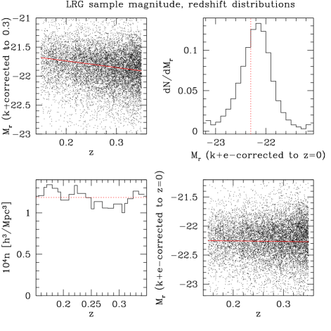
Model (not Petrosian) magnitudes were used for all luminosity cuts described in this paper; in all cases, $h=1$ magnitudes were used, so the division into samples does not depend on $h$. Magnitudes are corrected for extinction using reddening maps from Schlegel et al. (1998). We apply a k+e-correction (combined k-correction and correction for evolution of the spectrum) to all magnitudes to redshift zero as in Wake, et. al. (2006, in prep.) using the Bruzual & Charlot (2003) stellar population synthesis code. We note that if we do not use these k+e-corrections, but simply use kcorrect v4_1_4 (Blanton et al., 2003b) to the sample median redshift of 0.27, the resulting absolute magnitude histogram suggests that the galaxies above the median redshift are on average brighter than those below it. This result is consistent with the sign of passive evolution, for which galaxies are brighter in the past. In order to avoid our luminosity cuts selecting intrinsically different samples at high and low redshift, we apply all luminosity cuts using the k+e-corrected luminosities. Figure 3 shows information about the redshift and magnitude distribution of the sample.

In order to study variation with luminosity, we divide the sample into two subsamples at $M_{r}=-22.3$; roughly 2/3 of the sample is fainter than this value, and 1/3 is brighter, giving approximately equal signal to noise in each bin. Sample parameters are included in Table 2.

Figure 3: Upper left panel: scatter plot of absolute magnitude in $r$ band, k-corrected to $z=0.3$, versus redshift; line shows average trend with redshift (total change of 0.2 magnitudes across the full redshift range). Upper right: absolute magnitude distribution $dn/dM_{r}$ when k+e-corrected to $z=0$, with a line indicating the cut value between the faint and bright bins. Lower right: $M_{r}$ k+e-corrected to $z=0$ versus redshift; line shows average trend with redshift, which is nearly constant (total change of 0.02 magnitudes across the full redshift range). Lower left: comoving number density as a function of redshift, with a line indicating the average value.

Scale radii for the baryonic components were obtained by finding the average de Vaucouleurs profile fit radius for each sample from Photo, the SDSS processing pipeline; all radii quoted here are half-light radii.

For this paper, we isolate “host” versus “satellite galaxies” using spectroscopic galaxy counts in cylinders of comoving radius 2 $h^{-1}$Mpc and line-of-sight length $\Delta v=\pm 1200$ km s^-1. Since we only want to eliminate galaxies for which there is another, brighter spectroscopic LRG nearby, we simply require that those LRGs in our “host” sample either (a) be the only one in the cylinder, or (b) be the brightest in the cylinder.

A problem with this scheme is fiber collisions; since fibers cannot be placed closer than 55”, corresponding to 200 $h^{-1}$kpc at these redshifts, we may in principle still have some satellite galaxies that will distort the observed profile shape. Note that roughly 9 per cent of spectroscopic LRGs lack redshifts due to either fiber collisions, or due to redshift failure. We address this issue by using all galaxies passing the spectroscopic LRG sample cut I (below $z=0.36$) and the additional stringent color-magnitude cut from Loh & Strauss (2006, in prep.), whether or not a spectrum was obtained, in order to test whether a galaxy is a host or a satellite. For those LRGs without spectra, we used the redshift of the nearest LRG if there was one within 55”; otherwise, we used photometric redshifts from Kphotoz v4_1_4 with luminous red galaxy templates (Blanton et al., 2003b), with $\sigma_{z}\sim 0.03$ for these bright red galaxies. If the galaxy without a spectrum turned out to be brighter than a galaxy with a spectrum within a cylinder, we use the brighter one despite the lack of a spectrum. This cut on local environment reduces the sample by roughly 8 per cent.

Table 2: The lens samples used for this analysis, including redshift, absolute magnitude, stellar mass limits, and typical scale radii.

Sample	$N$	$z$ limits	$\langle z\rangle$	$z_{eff}$	$M_{r}$ limits	$\langle L/L_{\odot}\rangle$	$\langle M_{*}\rangle$	$r_{deV}$
						$h^{-2}10^{10}$	($10^{11}h^{-1}M_{\odot}$)	$h^{-1}$kpc
Faint LRGs	27 700	$[0.15,0.35]$	0.27	0.24	$M_{r}>-22.3$	5.2	2.2	8
Bright LRGs	15 635	$[0.15,0.35]$	0.27	0.24	$M_{r}\leq-22.3$	8.6	3.7	11

We obtained stellar mass estimates in the following way. First, we use the estimates from Padmanabhan et al. (2004), which found that $M_{stellar}/L\sim 3M_{\odot}/L_{\odot}$ for ellipticals (this is also consistent with the relationship between $M_{stellar}$ and $L$ seen in Mandelbaum et al. 2005d for bright red galaxies). The average luminosities of the faint and bright LRG samples determined in terms of $L_{\odot}$ using the absolute magnitude of stellar luminosity determined in Blanton et al. (2003c) are $5.2$ and $8.6h^{-2}\times 10^{10}L_{\odot}$ respectively, and with $L_{*}=1.2h^{-2}\times 10^{10}L_{\odot}$, we find (with appropriate factors of $h=0.7$) stellar masses of $2.2$ and $3.7\times 10^{11}h^{-1}M_{\odot}$, respectively.

Finally, we will further split the “bright” LRG sample at $M_{r}=-22.6$ in order to better trace the $M(L)$ relation. When this split is done, the $M_{r}<-22.6$ sample contains $1/9$ of the full LRG sample, and the $-22.3>M_{r}>-22.6$ sample contains $2/9$.

3.2 Sources

The source sample used is the same as that originally described in Mandelbaum et al. (2005a), hereinafter M05. This source sample includes over 30 million galaxies from the SDSS imaging data with $r$-band model magnitude brighter than 21.8, with shape measurements obtained using the REGLENS pipeline, including PSF correction done via re-Gaussianization (Hirata & Seljak, 2003) and with cuts designed to avoid various shear calibration biases. A full description of this pipeline can be found in M05; here we include only a brief summary.

The REGLENS pipeline obtains galaxy images in the $r$ and $i$ filters from the SDSS “atlas images” (Stoughton et al., 2002). The basic principle of shear measurement using these images is to fit a Gaussian profile with elliptical isophotes to the image, and define the components of the ellipticity

$$(e_{+},e_{\times})=\frac{1-(b/a)^{2}}{1+(b/a)^{2}}(\cos 2\phi,\sin 2\phi),$$ (16)

where $b/a$ is the axis ratio and $\phi$ is the position angle of the major axis. The ellipticity is then an estimator for the shear,

$$(\gamma_{+},\gamma_{\times})=\frac{1}{2\cal R}\langle(e_{+},e_{\times})\rangle,$$ (17)

where ${\cal R}\approx 0.87$ is called the “shear responsivity” and represents the response of the ellipticity (Eq. 16) to a small shear (Kaiser et al., 1995; Bernstein & Jarvis, 2002). In practice, a number of corrections need to be applied to obtain the ellipticity. The most important of these is the correction for the smearing and circularization of the galactic images by the PSF; Mandelbaum et al. (2005a) uses the PSF maps obtained from stellar images by the psp pipeline (Lupton et al., 2001), and corrects for these using the re-Gaussianization technique of Hirata & Seljak (2003), which includes corrections for non-Gaussianity of both the galaxy profile and the PSF. In order that these corrections can be successful, we require that the galaxy be well-resolved compared to the PSF in both $r$ and $i$ bands (the only ones used for shape measurement), where we define the Gaussian resolution factor

$$R_{2}=1-\frac{T^{(P)}}{T^{(I)}}$$ (18)

where the $T$ values are the traces of the adaptive covariance matrices, and the superscripts indicate whether they are of the PSF or of the galaxy image.

M05 includes a lengthy discussion of shear calibration biases in this catalog; we will only summarize these issues briefly here. Our source sample is divided into three subsamples: $r<21$, $r>21$, and high-redshift LRGs (Eisenstein et al., 2001), defined using color and magnitude cuts as in M05 using selection criteria related to those from Eisenstein et al. (2001) and Padmanabhan et al. (2005). Using simulations from Hirata & Seljak (2003) to estimate the PSF dilution correction and analytical models for selection biases and other issues that affect shear calibration, we place $2\sigma$ limits on the shear calibration bias of $[-0.05,0.12]$ for $r<21$, $[-0.08,0.18]$ for $r>21$, and $[-0.06,0.19]$ for LRGs.

As shown in Eq. 3, the lensing signal $\Delta\Sigma$ is a product of the shear and factors involving lens and source redshifts. Since the lenses have spectroscopic redshifts, the primary difficulty is determining the source redshift distribution. We take three approaches, all described in detail in M05. For the $r<21$ sources, we use photometric redshifts and their error distributions determined using a sample of galaxies in the Groth strip with redshifts from DEEP2 (Davis et al., 2003; Madgwick et al., 2003; Coil et al., 2004; Davis et al., 2005), and require $z_{s}>z_{l}+0.1$ to avoid contamination from physically-associated lens-source pairs. For the $r>21$ sources, we use redshift distributions from DEEP2. For the high-redshift LRGs, we use photometric redshifts and their error distributions determined using data from the 2dF-Sloan LRG and Quasar Survey (2SLAQ), and presented in Padmanabhan et al. (2005). Note that the LRG lenses used in this paper are typically at higher redshift than the lenses used in M05 and for this reason we are more sensitive to errors in the source redshift distribution. We will discuss the implications of this in §4.2.

Finally, we have placed constraints on other issues affecting the calibration of the lensing signal, such as the sky subtraction problem, intrinsic alignments, magnification bias, star-galaxy separation, and seeing-dependent systematics. As shown in M05 the calibration of the signal using the three source samples agrees to within 10 per cent, with a total $1\sigma$ calibration uncertainty estimated at 7 per cent ($r<21$) or 10 per cent ($r>21$ and LRG).

3.3 Signal computation

Here we describe the computation of the lensing signal. Lens-source pairs are assigned weights according to the error on the shape measurement via

$$w_{ls}=\frac{\Sigma_{c}^{-2}}{\sigma_{s}^{2}+\sigma_{SN}^{2}}$$ (19)

where $\sigma_{SN}^{2}$, the intrinsic shape noise, was determined as a function of magnitude in M05, figure 3. The factor of $\Sigma_{c}^{-2}$ downweights pairs that are close in redshift.

Once we have computed these weights, we compute the lensing signal in 53 logarithmic radial bins from 20 $h^{-1}$kpc to 4 $h^{-1}$Mpc as a summation over lens-source pairs via:

$$\Delta\Sigma(R)=\frac{\sum_{ls}w_{ls}\gamma_{t}^{(ls)}\Sigma_{c}}{2{\cal R}\sum_{ls}w_{ls}}$$ (20)

where the factor of 2 arises due to our definition of ellipticity.

There are several additional procedures that must be done when computing the signal (for more detail, see M05). First, the signal computed around random points must be subtracted from the signal around real lenses to eliminate contributions from systematic shear. Second, the signal must be boosted, i.e. multiplied by $B(R)=n(R)/n_{rand}(R)$, the ratio of the number density of sources relative to the number around random points, in order to account for dilution by sources that are physically associated with lenses, and therefore not lensed.

In order to determine errors on the lensing signal, we divide the survey area into 200 bootstrap subregions, and generate 2500 bootstrap-resampled datasets.

We also would like to account for the total calibration uncertainty of roughly 8 per cent at the $1\sigma$ level (including redshift uncertainties, shear calibration, stellar contamination, and all other effects that cause calibration bias). In principle, this can be done by multiplying the signal in each bootstrap resampled dataset by $1+0.08g$ where $g$ is a Gaussian random number with mean zero and variance $1$, and the net effect will be to cause correlations of order 8 per cent between radial bins in addition to any correlations due to shape noise, systematic shear, or other causes. However, we find that this procedure causes a significant bias in our fits, because points that are naturally below the best-fit signal have their errorbars increased by a smaller amount than those that are above the best-fit signal, and therefore those that are below the real signal are weighted more highly in the fits. Consequently, we generate the bootstrap-resampled datasets without including the calibration uncertainty, and add the 8 per cent uncertainty in quadrature with the statistical error on the mass determination.

Furthermore, to decrease noise in the covariance matrices due to the bootstrap, we rebin the signal into 18 radial bins total (of which 12 are in the range of radii that we will eventually elect to use for the fits).

3.4 Theoretical systematics

There are several theoretical systematics that are particularly problematic on small scales near massive galaxies. Here we describe two of them, estimate their magnitude, and explain how we correct for them.

3.4.1 Non-weak shear

The first small scale systematic we consider is the fact that for these relatively massive halos, the assumption of weak shear may no longer hold on the smallest scales that we probe (20 $h^{-1}$kpc). In reality, what is measured in g-g lensing measurements is the reduced shear,

$$g_{t}=\frac{\gamma_{t}}{1-\kappa},$$ (21)

(where $\kappa=\Sigma/\Sigma_{c}$). Hence, $g_{t}\approx\gamma_{t}$ to a high degree of accuracy in the $\gamma_{t}\ll 1$, $\kappa\ll 1$ regime that is typically probed with weak lensing. Fig. 4 includes a plot of $\gamma_{t}$, $\kappa$, and $g_{t}$ for a typical LRG profile with the same density profile parameters as in Fig. 1, without adiabatic contraction (AC makes no perceptible difference in these quantities on these scales). As shown there, at the minimum scale at which we attempt to measure the lensing signal (20 $h^{-1}$kpc) the difference between $\gamma$ and $g$ is $\sim 15$ per cent, and at 40 $h^{-1}$kpc it is 9 per cent, causing us to overestimate $\Delta\Sigma$.

Figure 4: $\kappa$, $\gamma_{t}$, and $g_{t}$ for the typical density profile described in the text, as labelled on the plot.

Unfortunately, it is difficult to take into account the effect of non-weak shear on our shear estimator, $\langle e_{+}\rangle$, in a way that is completely model-independent. Appendix A shows the rather involved calculations necessary to estimate the importance of any terms beyond first-order in $\gamma_{t}$ and $\kappa$. As we show there (Eq. 53, reproduced here for convenience), the second-order calculation of the value of the shear estimator is

$$\langle e_{+}\rangle=2{\cal R}\langle\Delta\Sigma\rangle\langle\Sigma_{c}^{-1}\rangle\left(1+\frac{\langle\Delta\Sigma\,\Sigma\rangle}{\langle\Delta\Sigma\rangle}\frac{\langle\Sigma_{c}^{-2}\rangle}{\Sigma_{c}^{-1}}\right),$$ (22)

which gives a correction larger than the naive $1+\kappa$.

The two fractions in the correction term need to be estimated in some manner. The first one can be estimated using our earlier model of averaging $\Delta\Sigma$ over the halo mass function from the relevant minimum mass to the maximum mass, and is found to be $\approx 1$ for the faint LRG sample, and $\approx 1.03$ for the bright LRG sample. The second fraction in the correction term, $\langle\Sigma_{c}^{-2}\rangle/\langle\Sigma_{c}^{-1}\rangle$, can be very simply calculated when the signal is calculated, where the averages are computed using the weighting used to get the lensing signal, and typically equals approximately 1.05. Then, when the fitting is completed, we multiply the model $\Delta\Sigma$ by the correction term.

3.4.2 Magnification bias

The next issue we consider is the effect of magnification bias on the boost factors. Magnification bias will tend to increase or decrease the number density of observed sources relative to that expected from the random catalogs; hence, our procedure of multiplying the signal by $n(R)/n_{rand}(R)$ in order to correct for dilution by physically associated (non-lensed) sources will tend to overestimate the signal, since some of those additional sources are actually lensed. The degree of this overestimation was computed for each source sample as a function of its apparent magnitude and resolution factor distributions, and was found in M05 to be $\delta n/n=1.9\kappa,0.7\kappa,3.1\kappa$ for $r<21$, $r>21$, and LRG sources respectively. (Note that $\langle\Sigma_{c}^{-1}\rangle$ varies with source sample as well, which gives different $\kappa$ for each sample.) In order to correct for this overestimation, we multiply the signal for each model by $(1+a\Sigma\langle\Sigma_{c}^{-1}\rangle)$ before comparing against the real data, where $a$ and $\langle\Sigma_{c}^{-1}\rangle$ are found as a weighted average over the values for each source sample. Fig. 4 shows, for the model density profile used throughout this section, the value of $\kappa$ from which the size of this correction factor can be ascertained.

A related issue is that of the effect of magnification bias on the source redshift distribution. This effect is not a problem for the $r<21$ or the LRG source sample, since we use photometric redshifts that should still be reliable, so it is only a concern for the $r>21$ sample for which we use a distribution $p(z)$. Since magnification bias allows the observation of sources that would not have otherwise been seen, it means that in regions where magnification bias is significant, we tend to underestimate the source redshifts, and therefore $\Sigma_{c}^{-1}$, overestimating the signal $\Delta\Sigma$. The mean redshift of the $r>21$ sample is $\langle z\rangle=0.45$.

For the model LRG signal used in this section, we estimate the size of this effect as follows. We consider a moderately large value of $\kappa=0.1$ such as may be present for transverse separations of 40 $h^{-1}$kpc (see Fig. 4). For the $r>21$ sample, this means that $\delta n/n~{}0.07$, so the fraction of sources used that have been scattered into the sample is $0.07/1.07\sim 0.065$. We consider what happens if those sources are actually all at $z=1$ (more than twice the mean redshift of this sample, giving a conservative estimate). $\Sigma_{c}^{-1}$ for these sources is then actually 50 per cent larger than what we have assumed. If 6.5 per cent of the sample has had its $\Sigma_{c}^{-1}$ value so underestimated, this means that the sample average $\Sigma_{c}^{-1}$ value is thus 3 per cent too small, and the signal has been overestimated by this amount. Since this value is far smaller than other sources of systematic and statistical error, and is a conservative estimate, we do not apply a correction.

4 Results

Those who are uninterested in the details of the lensing systematics tests in the following subsections may wish to skip directly to the results of the fitting, in subsection 4.4.

4.1 Small-scale software-related systematics

One systematic potentially affecting all source samples on small scales is the sky subtraction systematic, an error in the sky estimation near bright lenses (Mandelbaum et al., 2005a; Adelman-McCarthy et al., 2006). A similar systematic is the possibility of errors in deblending. To test for these problems, we use simulations that were used for the small-scale LRG autocorrelation function measurement in Masjedi et al. (2005). These simulations were created by placing fake LRGs on real SDSS images in run 2662, camcol 1. For that paper, the issue of concern was the effect on a measured LRG flux due to the presence of another nearby LRG, so two fake LRGs were placed in each field at various angular separations. For this work, similar simulations were created with only one fake LRG per SDSS field, with 470 fields total. The simulated LRG flux is $r=17.9$, corresponding to a $M_{r}=-22.5$ LRG at $z=0.3$ with $r_{deV}=3.4$”. The axis ratio $b/a=0.7$, with quantized random orientation relative to the scan direction (i.e., it was allowed to have any of 360 orientations evenly spaced in position angle). We used these values of flux and size to place conservative constraints on software-induced systematics; studying the variation with LRG size and flux is unfortunately prohibitive due to computer time and storage space limitations.

The new images were then processed with the same version of the SDSS processing software, Photo, as the original data (rerun 137). We use these results to decide which ranges of transverse separations to use in the real data. The results presented in this paper are averaged over five separate “reruns” with different simulated LRG positions but the same photometric properties.

There are several concerns for which we would like to test:

1. Over- or under-estimation of the sky can lead to modulation of the number density near LRGs (because they change the flux and apparent size, and hence scatter galaxies into or out of our catalog). Since we assume that any change in number density relative to that around random points is due to physically-associated sources, this problem may cause a bias in the lensing signal.

2. If the deblender or sky determination algorithm includes a spurious gradient in the flux around LRGs, it can lead to the galaxies near the LRG (whether physically-associated or not) having some spurious additive and/or multiplicative shear.

3. If the LRGs cause nearby galaxies to have mis-measured fluxes, then depending on the way this effect varies with band, it may change the colors and hence lead to inaccurate photometric redshift determination. This problem would affect the $r<21$ and LRG source samples. Furthermore, for the $r>21$ sample, for which we assume $dn/dz$, the redshifts of the sources may be underestimated, and hence $\Delta\Sigma$ overestimated, by some amount.

In order to test for these effects, we searched for real galaxies around the positions of the simulated LRGs in the real data and the simulations. The first test, for modulation of number density, was performed simply by comparing the number of real galaxies around those locations in the simulation versus in the real data; results are shown in the upper left panel of Fig. 5.

Figure 5: Four plots showing the effect of simulated LRGs on real galaxies in SDSS data. In all plots, the dotted line shows the nominal value if the simulated LRGs had no effects on the photometry of the real galaxies. The upper left panel shows the effect on the number density of real galaxies in our lensing source catalog around the positions of fake LRGs. The upper right panel shows the effect of the simulated LRG on the real galaxy fluxes in both $r$ and $i$ bands as labelled. The lower left panel shows the effect on the apparent size of the real galaxies relative to the size of the PSF, where the quantities measured are described in more detail in the text. Finally, the lower right panel shows the spurious shear caused by the deblender or the sky subtraction errors; in order to make the results easier to view, this quantity has been multiplied by $(\theta/10^{\prime\prime})^{2}$.

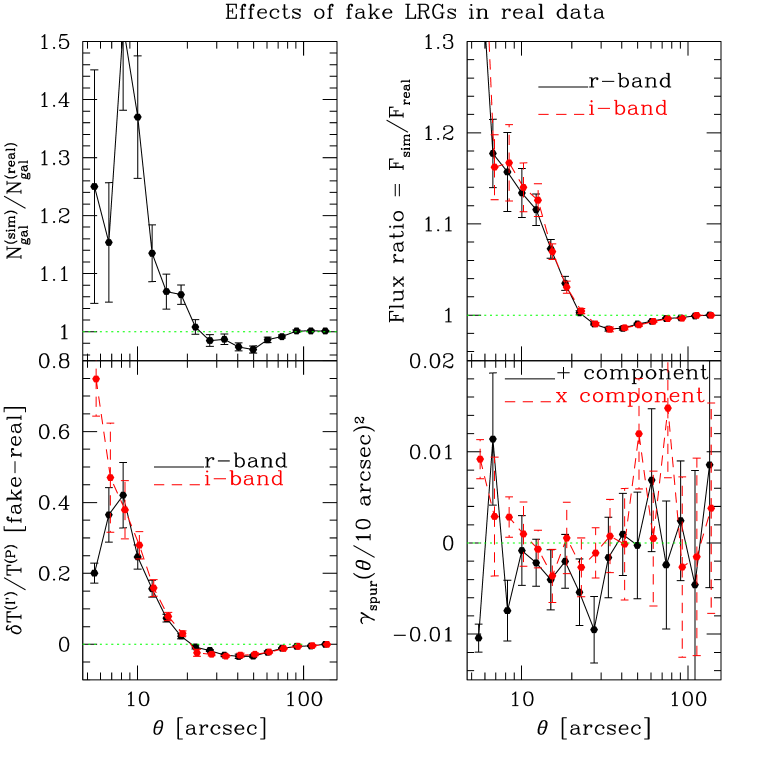
As shown there, there is the same depletion in number density on 30–90^′′ scales as noted in previous works, with a crossover point occuring between 20–30^′′, and an excess of galaxies below that point. These findings are consistent with the sky being underestimated (and hence source galaxy fluxes overestimated) below the crossover point, and overestimated above that point. We note that the crossover point around $23^{\prime\prime}$ corresponds to $\sim 93$ comoving $h^{-1}$kpc at the sample mean redshift. Also, in this panel as for the others, the results in the simulations match those in the real data above $100^{\prime\prime}$.

Next, we calculated both the tangential and 45 degree shear components around the positions of the fake LRGs, using only those real galaxies that passed cuts to be in our source catalog in both the real data and the simulation. The importance of this cut is that if we use the same real galaxies in both samples, then when we take the difference between the shears in these samples, all shape noise will be eliminated, giving an estimate of the “systematic” shear in both components. The resulting plot is shown in the lower right panel of Fig. 5. The $x$ shear component, while containing several points that are slightly discrepant from zero, is nonetheless consistent with zero spurious shear for all points above 10”; below this scale, the errorbars on both shear components appear to be underestimated. The $+$ shear component, the tangential shear, is also consistent with zero down to 10”, or roughly 40 $h^{-1}$kpc: the constraint $|\gamma_{sys}|<0.004$ corresponds to $|\Delta\Sigma_{sys}|<20$, which is far smaller than the statistical errors. Below this scale, constraints on contamination are weaker, so we use a minimum transverse separation of $40$ $h^{-1}$kpc for all fits.

This calculation only shows additive shear on galaxies that are matched. In the real data, any additive shear determined in this way will have to be multiplied by the boost factor $B(R)$, since physically-associated sources are equally susceptible to software-induced systematics. Furthermore, this calculation only applies to galaxies that are matched in both the real and simulated data; it does not apply to galaxies that are scattered into the catalog due to sky underestimation. It is plausible that there is some selection bias operating in the selection as these galaxies, for instance causing us to select those that are aligned tangentially to the lens rather than radially, that would cause an additional bias in the results. Unfortunately, placing constraints on these galaxies is much more demanding because there are no matching galaxies in the real data with which they can be paired to eliminate shape noise. Finally, this calculation tells us about additive shear errors, but not about multiplicative biases due to the deblender.

The next question we address is that of the effect on the fluxes. While it is clear that either the fluxes or apparent sizes of sources near the fake LRGs is affected (since the number density of sources changes near them), the change in the fluxes may also affect classification into our three source samples, and may change photometric redshifts for the two samples that use them and the source redshift distribution for the $r>21$ sample. For the galaxies that match in the real versus simulated data, the upper right panel of Fig. 5 shows the ratio of measured flux in the simulated data versus in the real data, in both $r$ and $i$ bands. As shown, at 10” ($\approx 40h^{-1}$kpc), the fluxes are overestimated by roughly 15 per cent, corresponding to a change in apparent magnitude of 0.15. Interestingly enough, the change is consistent for the $r$ and $i$ bands, even though the simulated LRG fluxes in these bands are not the same. This suggests that the effect may not noticably change photometric redshifts since they depend on color rather than magnitude.

Finally, while we may guess that the change in number density is only due to the shift in the apparent magnitudes, the lower left panel of Fig. 5 indicates that the apparent sizes of the galaxies relative to the sizes of the PSF are also changed in a way that can cause the number densities to change as in the upper left panel. The quantity shown in this plot is

$$\frac{T^{(I)}_{sim}-T^{(I)}_{real}}{T^{(P)}}=\frac{\delta T^{(I)}}{T^{(P)}},$$ (23)

or the change in the trace of the adaptive moment matrix due to presence of the LRG, relativev to the trace of the adaptive moment matrix of the PSF. When we compare against Eq. 18, we see that the change in resolution factor $R_{2}$ due to the change in apparent size is

$$\delta R_{2}=\frac{\delta T^{(I)}}{T^{(P)}}(1-R_{2})^{2}$$ (24)

So, for a typical galaxy with $R_{2}=0.55$ (sample median) at 10” from one of these LRGs, the resolution factor is increased by 0.09 to 0.64. A typical galaxy at separations of 60” has resolution factor decreased by -0.01 to 0.54.

Finally, we note for the sake of completeness that this simulation was only for one type of LRG, $r=17.9$, with $r_{deV}=3.3$”. This is reasonably close to the mean apparent magnitude of the spectroscopic LRGs used for this analysis. We have not derived variations of the effect with total LRG flux or apparent size, nor have we done any calculations for galaxies with profiles that are not purely de Vaucouleurs, so these results should not be used for, e.g., the Main galaxy sample which has a higher flux on average, and is a mixture of both de Vaucouleurs and exponential profile galaxies.

As a result of the findings in this section that deblending and sky subtraction systematics become significantly worse in a way that is difficult to quantify below about 10” (or 40 $h^{-1}$kpc), in the analysis that follows, we only use the lensing signal above 40 $h^{-1}$kpc for fits even though plots show signal down to 20 $h^{-1}$kpc . We correct the signal for the overestimation of the boosts due to the modulation of the number density near the LRGs, but because this correction is so large and uncertain below 10”, we only show the results below that separation to demonstrate consistency with the results derived from higher angular separations. We also increase the error bars to account for systematics, with an increase of 50 per cent at 20 $h^{-1}$kpc down to no increase at 50 $h^{-1}$kpc.

4.2 Signal amplitude

In this section we discuss the lensing signal calibration for each source sample. The standard systematics tests as described in Mandelbaum et al. (2005a) were performed to ensure that systematics are under control (45-degree test, random catalog test), and no anomalies were found.

One test that we focus on in particular here is the ratio test, which allows us to compare the effective average amplitude of $\Delta\Sigma$ for different source samples. The ratio test is of particular interest because, for Mandelbaum et al. (2005a), the lensing signal for the three source samples was found to be consistent at the $1\sigma$ level, but with lenses at a median redshift of $0.1$. For this work, the lens redshift range is from $0.15$ to $0.35$, with an effective mean of $0.24$. The peak redshift of the $r<21$ sample is $0.35$, quite close to the lenses, which means that for this work, we are far more sensitive to the details of the photometric redshift error distribution than for Mandelbaum et al. (2005a). In contrast, the mean redshift of the $r>21$ sample is $0.45$ and of the LRG source sample is $0.55$, so we expect that the signal with these two source samples will still be fairly reliable.

Figure 6: Lensing signal $\Delta\Sigma$ for the bright lens sample, with three different source samples as indicated on the plot.

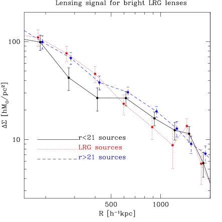
Fig. 6 shows the lensing signal for the bright LRG lens sample with the $r<21$, $r>21$, and LRG source samples separately for $150<R<2000$ $h^{-1}$kpc. We use these scales because they are the most free of systematics and offer the highest signal-to-noise. It seems clear that the LRG and $r>21$ samples effectively agree in average amplitude, but the $r<21$ sample gives a lower overall calibration. When we determine an average effective amplitude of the lensing signal for each lens sample (“faint,” “bright,” and “all”) for each bootstrap dataset, and compare this amplitude for the different source samples, we find the following relations hold:

$$\frac{\langle\Delta\Sigma\rangle_{r>21}}{\langle\Delta\Sigma\rangle_{LRG}} =0.98\pm 0.11, \frac{\langle\Delta\Sigma\rangle_{r<21}}{\langle\Delta\Sigma\rangle_{r>21}} =0.84\pm 0.11\mbox{ (faint)}$$ (25)

$$\frac{\langle\Delta\Sigma\rangle_{r>21}}{\langle\Delta\Sigma\rangle_{LRG}} =1.01\pm 0.09, \frac{\langle\Delta\Sigma\rangle_{r<21}}{\langle\Delta\Sigma\rangle_{r>21}} =0.86\pm 0.08\mbox{ (bright)}$$ (26)

$$\frac{\langle\Delta\Sigma\rangle_{r>21}}{\langle\Delta\Sigma\rangle_{LRG}} =1.00\pm 0.07, \frac{\langle\Delta\Sigma\rangle_{r<21}}{\langle\Delta\Sigma\rangle_{r>21}} =0.85\pm 0.06\mbox{ (all)}$$ (27)

As shown in Eq. 25, the signal for the LRG and $r>21$ source samples is statistically consistent for both LRG lens samples, but in contrast, the signal with the $r<21$ (photoz) sources is about 15 per cent lower, a $2.5\sigma$ discrepancy when considering all lenses together. This finding suggests that for the $r<21$ sample, some problem with the photometric redshift error distributions is causing $\Sigma_{c}^{-1}$ to be overestimated by 15 per cent, thus underestimating $\Delta\Sigma$ by that amount.

In order to test this hypothesis, we further split the $r<21$ sources into two samples: those with photometric redshift lower than $0.4$, and those with photometric redshift higher than $0.4$. When we compare the signal with the “low redshift” and “high redshift” $r<21$ sources, we find the following relations:

$$\frac{\langle\Delta\Sigma\rangle_{z_{s}>0.4}}{\langle\Delta\Sigma\rangle_{z_{s}<0.4}}=\begin{cases}0.71\pm 0.13,&\text{Faint LRG lenses;}\\ 0.80\pm 0.12,&\text{Bright LRG lenses;}\\ 0.76\pm 0.09,&\text{All LRG lenses.}\end{cases}$$ (28)

The net result, then, is that the sources with photometric redshift larger than $0.4$ give signal that is 24 per cent lower than the signal with photometric redshift lower than $0.4$. When we take into account that this higher photometric redshift sample has more weight than the lower photometric redshift sample, this explains the signal with the full photometric redshift sample being low by 15 per cent. This result also explains our failure to notice this discrepancy in previous works; for Mandelbaum et al. (2005a) and Mandelbaum et al. (2005d), the mean lens redshift was lower, so (a) the sample with photometric redshift lower than $0.4$ had significantly higher weight than the sample with photometric redshift greater than $0.4$; and (b) an imperfect understanding of the photometric redshift bias and scatter at photometric redshift larger than $0.4$ gives a smaller fractional error on $\Sigma_{c}^{-1}$ for lower lens redshift. Consequently, the signal with the $r<21$ sample was not as noticably discrepant in previous works.

When considering $\Sigma_{c}^{-1}(z_{l}=z_{eff},z_{s})$ as a function of source redshift, we note that for galaxies at $r<21$, a net bias of 0.04 would be sufficient to achieve a 15 per cent change in overall calibration, e.g. if we assume that galaxies really at $z=0.4$ are at $z=0.44$. Alternatively, a smaller bias of $\sim 0.02$ and a modest increase in the net scatter of $0.02$ will tend to cause the same change in calibration. Since the peak of the redshift distribution for these galaxies is around $z=0.35$, the photometric redshift error distribution was determined with a large number of galaxies from $z=0.3$–$0.4$, but with a much smaller number of galaxies at $z>0.4$, and hence a bias and scatter increase of these magnitudes is within the statistical error.

Considering that we can fairly easily explain this bias in the $r<21$ sample relative to the more reliable (for this purpose) $r>21$ and LRG source samples, before doing the fits we have increased the signal with the $r<21$ sample by 15 per cent as in Eq. 25, and increased the statistical error by 6 per cent to account for the statistical error in the determination of this calibration factor. In practice, the increase in statistical error is achieved by multiplying the signal in individual bootstrap samples by a random number of mean $1$ and Gaussian standard deviation $0.06$. Note that this calibration change affects the mass determination, not the profile shape.

4.3 Intrinsic alignments

There are two intrinsic alignment effects that are important for lensing, but only one is important for galaxy-galaxy lensing as presented here. The intrinsic ellipticity-intrinsic ellipticity (II) correlation is not important for galaxy-galaxy lensing, because we average over all relative lens-source ellipticity orientations. The second effect, which is important for this work, is an alignment between the intrinsic ellipticity and the local density field, or the GI correlation. This effect comes into play because we necessarily include some physically-associated pairs (i.e., pairs of lenses and “sources” that are really part of the same local structure), so if those sources have a tendency to align tangentially or radially relative to the lens, they will provide an additive bias to the lensing signal.

Correlations between intrinsic ellipticity and density have been demonstrated robustly using bright, red galaxies on large scales (Mandelbaum et al., 2006) and on small scales (Mandelbaum et al., 2005c; Donoso et al., 2006; Yang et al., 2006), with the effect being more controversial for the general galaxy population and for spirals. In the cases considered in these papers, the typical scenario is that a large, bright galaxy is found to point preferentially in the direction of nearby overdensities, e.g., along a cluster major axis. In our case, we are concerned that the fainter sources around a large, bright galaxy may be pointing preferentially radially or tangentially towards it; unfortunately, constraints on this scenario are weak and/or difficult to convert to measurements of lensing shear (Lee & Pen, 2001; Bernstein & Norberg, 2002; Hirata et al., 2004). We expect that on scales larger than $\sim 100$ $h^{-1}$kpc, above which the boost factors are fairly small, there will be little contribution from intrinsic alignments.

Here, we try to measure the intrinsic alignment contamination of the lensing signal using photometric redshifts. For a given lens, the sources with $r<21$ are split into a “physically associated” (PA) sample with $z_{l}-0.1<z_{s}<z_{l}+0.1$ and a “lensed” (L) sample with $z_{s}\geq z_{l}+0.1$. The difficulty, of course, is that the photometric redshifts have a broad error distribution, so that both of these samples are going to have some galaxies in them that do not actually fit the criteria of being PA or L; in the two samples, the fractions of physically associated sources are $f_{PA}^{(PA)}=(B^{(PA)}-1)/B^{(PA)}$ and $f_{PA}^{(L)}=(B^{(L)}-1)/B^{(L)}$. We measure signals $\hat{\gamma}^{(PA)}$ and $\hat{\gamma}^{(L)}=\Delta\Sigma^{(L)}\langle\Sigma_{c}^{-1}\rangle^{(L)}$ that are related to the “real” lensing and PA shears via

$$\hat{\gamma}^{(PA)} =f_{PA}^{(PA)}\gamma_{PA}^{(PA)}+(1-f_{PA}^{(PA)})\gamma_{L}^{(PA)}$$ (29)

$$=f_{PA}^{(PA)}\gamma_{PA}^{(PA)}+(1-f_{PA}^{(PA)})\Delta\Sigma_{L}^{(L)}\langle\Sigma_{c}^{-1}\rangle^{(PA)}$$

where the lensing shear in the PA sample can be determined using $\Delta\Sigma$ from the lensing signal and multiplying by the average $\Sigma_{c}^{-1}$ for the PA sample. This average value can be determined by integrating over the known lens redshift distribution, source photometric redshift distribution, and photometric redshift error distribution, and is found to be a factor of $2.5$ lower than $\langle\Sigma_{c}^{-1}\rangle^{(L)}$, partly due to the significant number of sources in the PA sample that are foregrounds wth $\Sigma_{c}^{-1}=0$. Thus, we can rearrange this equation to get $\gamma_{PA}^{(PA)}$, the intrinsic alignment shear in the PA sample, from the measured shear with the physically assocated sample.

Next, we can estimate the contamination to the real lensing signal using the following equation:

$$\hat{\gamma}^{(L)} =B^{(L)}\left[(1-f_{PA}^{(L)})\gamma_{L}^{(L)}+f_{PA}^{(L)}\gamma_{PA}^{(L)}\right]$$ (30)

$$=\gamma_{L}^{(L)}+\frac{f_{PA}^{(L)}}{1-f_{PA}^{(L)}}\gamma_{PA}^{(L)}$$ (31)

We note several things about this equation. The first term is simply the lensing signal, where the boost factor is necessary to account for the fact that not all the sources are lensed. The second term is the intrinsic alignment contamination term. We have pointed out with our notation a nuance that may be important: in Eq. 4.3, we will be able to determine the intrinsic alignment shear due to physically associated sources in the PA sample; in Eq. 31, we actually need the intrinsic alignment shear due to physically associated sources in the L sample. We return to this difference shortly.

Figure 7: Measured shear with the PA source sample for both LRG lens samples, and the implied shear due to intrinsic alignments after subtracting off the contribution due to lensing.

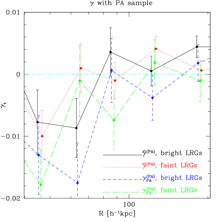
Fig. 7 shows the measured shear with the PA samples, $\hat{\gamma}^{(PA)}$ for the two lens samples, and then the corrected $\gamma_{PA}^{(PA)}$ after we remove the contamination due to lensing. As shown, the signals are consistent with zero above 100 $h^{-1}$kpc; below that scale, they are consistently negative, indicating a tendency for satellites to “point” radially towards primaries. The $\chi^{2}$ for a fit to zero signal for the two lens samples are $11.6$ and $12.5$ for the bright and faint lens samples respectively (with 3 degrees of freedom with $40<R<100$ $h^{-1}$kpc), giving a probability to exceed by chance of 0.01 and 0.007, indicating a positive detection on these scales. If we average the value of $\gamma_{PA}^{(PA)}$ for those scales, we get averages of $-0.0084\pm 0.0034$ and $-0.0086\pm 0.0030$. We can also get the projected lensing contamination, if we make the crucial assumption that $\gamma_{PA}^{(PA)}=\gamma_{PA}^{(L)}$, by using $\langle\Sigma_{c}^{-1}\rangle$ for the $r<21$ sample of $1.9\times 10^{-4}$. This signal, when subtracted from the measured $\hat{\gamma}^{(L)}$ to get a decontaminated lensing signal, leads to an increase of the signal roughly equivalent to the size of the $1\sigma$ errors or larger on these scales, and hence has a significant effect on fits to the profile.

In comparison with recent works, we note that using SDSS data, Agustsson & Brainerd (2005) also found a tendency for satellites to align radially towards primaries using spectroscopically-determined primary-satellite pairs. Over the range $7<R<50$ $h^{-1}$kpc, they found a mean tangential shear of $\gamma_{t}=-0.030\pm 0.007$. This number is, as expected, larger than our measured tangential shear, since ours is at a mean transverse separation that is close to three times as high as the mean separation for their measurement.

However, we must consider further whether this is really the proper correction to apply. For the $r<21$ sample, the sources that are truly physically associated in the L sample are, by definition, those with poor photometric redshifts. Hence, studies of the photometric redshifts that we use in comparison with DEEP2 redshifts (Mandelbaum et al., 2005a) indicate that these will tend to be, on average, bluer and fainter. On the other hand, the physically associated sources in the PA sample are those with good photometric redshifts, which will tend to be brighter and redder. There is no a priori reason to suppose, then, that $\gamma_{PA}^{(PA)}=\gamma_{PA}^{(L)}$, in light of the fact that many intrinsic alignment measurements indicate that the effect depends sensitively on the galaxy luminosity and color. In fact, both large- and small-scale measurements seem to indicate that intrinsic alignments are negligible for bluer, fainter galaxies and large for bright, red ones, which suggests that $\gamma_{PA}^{(L)}$ may well be zero, with no correction necessary (Azzaro et al., 2006; Mandelbaum et al., 2006; Yang et al., 2006).

The bottom line, then, is that it is not clear how to correct the signal with $r<21$ sources for intrinsic alignment contamination in a way that is not based on many tenuous assumptions. We may come to a similar conclusion about the $r>21$ sample. Since we only have a redshift distribution for this sample, the sample of galaxies that are physically associated are a mix of blue and red, but are on average (at a given redshift) fainter than the physically associated sources from the $r<21$ sample, and hence the corrections derived from the $r<21$ PA sample may not apply.

Because of this problem with both the $r<21$ and the $r>21$ samples with respect to intrinsic alignments on $R<100$ $h^{-1}$kpc scales, we choose to rely solely on the high-redshift LRG sources on these scales. While the high-redshift LRG sample contains, by definition, bright red galaxies that may be expected to have strong intrinsic alignments, they are located at redshifts $z>0.4$, whereas our lenses are in the range $0.15<z<0.35$. Furthermore, we impose a cut on the source photometric redshift ($z_{s}>z_{l}+0.1$) to further eliminate low-redshift contamination. The net effect is that the physically associated fraction at $R>40$ $h^{-1}$kpc is negligible when using this source sample, so it must be free of intrinsic alignments. To ensure that the signal on $40$–$100$ $h^{-1}$kpc scales, which may be crucial to understanding the profile, is as free of systematics as possible (while retaining higher statistical power on larger scales), we thus use only the LRG sources at $R<100$ $h^{-1}$kpc, and average all the source samples for $R>100$ $h^{-1}$kpc.

4.4 Fits to lensing signal

We begin the fits with the simplest possible way, and add parameters until the best-fit $\chi^{2}$ does not decrease with the addition of parameters. Table 3 shows the results for best-fit parameters for the fits as enumerated and described there. In this table, in all cases the fits are from a minimum scale of $40$ $h^{-1}$kpc (to avoid systematics-dominated inner regions) to a maximum of $2$ $h^{-1}$Mpc (to avoid the need for complicated modeling of the halo-halo term). Errors on all parameters are the formal $1\sigma$ errors from the fit covariance matrix determined using derivatives of the $\chi^{2}$ with respect to each fit parameter. We remind the reader that the mass estimates have had an additional 8 per cent systematic error added in quadrature with the formal statistical error, and the fits are performed using the full covariance matrix (which includes minimal correlations at small scales, and correlations as large as 20–30 per cent at large scales).

Table 3: Fits performed, including identifying number, and fit parameters. Bold-faced fit parameters are meant to indicate that they were held fixed, whereas those in regular font are those that were allowed to vary, with $1\sigma$ errors. For all fits, $R_{min}=0.04$ $h^{-1}$Mpc. Note that the fitted values for concentration should be increased by about 20 per cent when compared to simulations to account for the scatter in cluster profiles, which was found to reduce the value in the lensing fits. Similarly, the fitted masses correspond better to the median rather than mean mass (Mandelbaum et al., 2005b).

Fit	Description	$\alpha$	$\beta$	$c$	$M$	$M_{stellar}$	$R_{s}$	$\chi^{2}$	dof
					$10^{13}h^{-1}M_{\odot}$	$10^{11}h^{-1}M_{\odot}$	$h^{-1}$kpc
Faint LRG sample
1	SIS	$\mathbf{-2.0}$	$\mathbf{2.0}$	$\mathbf{10^{4}}$	$2.4\pm 0.3$	$\mathbf{2.2}$	$\mathbf{8}$	$18.6$	$10$
2	Power-law	$\mathbf{-2.0}$	$1.85\pm 0.06$	$\mathbf{10^{4}}$	$3.0\pm 0.4$	$\mathbf{2.2}$	$\mathbf{8}$	$11.5$	$10$
3	NFW	$\mathbf{-1.0}$	$\mathbf{3.0}$	$4.0\pm 0.6$	$2.9\pm 0.4$	$\mathbf{2.2}$	$\mathbf{8}$	$11.5$	$10$
4	NFW	$-0.50\pm 0.18$	$\mathbf{3.0}$	$\mathbf{7.7}$	$2.7\pm 0.4$	$\mathbf{2.2}$	$\mathbf{8}$	$13.8$	$10$
5	NFW	$\mathbf{-1.0}$	$2.5\pm 0.1$	$\mathbf{7.7}$	$2.9\pm 0.4$	$\mathbf{2.2}$	$\mathbf{8}$	$10.1$	$10$
Bright LRG sample
6	SIS	$\mathbf{-2.0}$	$\mathbf{2.0}$	$\mathbf{10^{4}}$	$5.6\pm 0.6$	$\mathbf{3.7}$	$\mathbf{13}$	$28.6$	$10$
7	Power-law	$\mathbf{-2.0}$	$1.85\pm 0.05$	$\mathbf{10^{4}}$	$7.8\pm 1.1$	$\mathbf{3.7}$	$\mathbf{13}$	$16.7$	$10$
8	NFW	$\mathbf{-1.0}$	$\mathbf{3.0}$	$4.7\pm 0.6$	$6.7\pm 0.8$	$\mathbf{3.7}$	$\mathbf{13}$	$10.5$	$10$
9	NFW	$-0.72\pm 0.12$	$\mathbf{3.0}$	$\mathbf{6.7}$	$6.4\pm 0.8$	$\mathbf{3.7}$	$\mathbf{13}$	$11.9$	$10$
10	NFW	$\mathbf{-1.0}$	$2.7\pm 0.1$	$\mathbf{6.7}$	$6.8\pm 0.8$	$\mathbf{3.7}$	$\mathbf{13}$	$9.4$	$10$

4.4.1 Faint LRG sample

Accordingly, we begin by discussing the results for the faint LRG sample, with the simplest fit performed, that for a simple SIS with fixed stellar component, with only one free parameter. This fit (fit number 1 in Table 3), along with several of the others to be discussed, appears in Fig. 8 with the measured signal. We have forced the profile in Eq. 6 to approximate a SIS by making $r_{s}$ very small, so that the logarithmic slope is equal to $-\beta=-2$ for the entire radial range of interest. It appears from the top panel of Fig. 8 that the model overestimates the signal on $40$–$80$ $h^{-1}$kpc scales.

Figure 8: Lensing signal for the faint LRG lens sample averaged over source sample, and best-fit signals. The vertical dotted line at 40 $h^{-1}$kpc shows the minimum scale used for the fits, and at $800$ $h^{-1}$kpc shows $r_{vir}$. The line types for each fit are indicated on the plot itself. We note that the signal shown here has been corrected for errors in the boost factor due to the sky subtraction error, but non-weak shear effects and magnification bias effecs on the boost factor are still incorporated in both the real and the model signal shown here. Errorbars are slightly correlated (20–30 per cent level) on large scales.

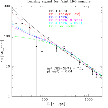
Next, we consider the results for a general single power-law, fit 2. The addition of a single additional parameter, the exponent of the power-law ($-\beta$), decreases the $\chi^{2}$ value by $7.1$ to $11.5$ relative to fit 1, despite the fairly small change in exponent from $-2$ to $-1.85\pm 0.06$, suggesting that the addition of this fit parameter is justified. To properly evaluate the goodness of this fit relative to that for the SIS using the $\Delta\chi^{2}$ value, we must take into account that it was calculated using a bootstrap covariance matrix, and as shown in Appendix D of Hirata et al. (2004), the expected $\chi^{2}$ values are not drawn from a $\chi^{2}$ distribution in this case. The probability value associated with exceeding this value of $\Delta\chi^{2}$ by chance is $p(>\Delta\chi^{2})=0.04$. On Fig. 8, it is apparent that this model is preferred over the SIS because it does not overestimate the signal on $40$–$80$ $h^{-1}$kpc scales as much as the SIS (though the model signal is slightly high on $1$–$2$ $h^{-1}$Mpc scales).

We then consider the simplest NFW-type fit, number 3, which has the same number of fit parameters as the single power-law, and the same $\chi^{2}$. Consequently, like the single power-law profile, the NFW model is preferred relative to the SIS at the 96 per cent CL. Visually, Fig. 8 suggests that particularly on $40$–$80$ $h^{-1}$kpc and $1$–$2$ $h^{-1}$Mpc scales, the NFW model is preferred. The best-fit value of mass, $(2.9\pm 0.4)\times 10^{13}h^{-1}M_{\odot}$. This should be compared to the median mass of the sample Mandelbaum et al. (2005b). It is lower than the value expected naively from the halo mass function using high normalization, in Table 1; it is close to the predicted lower mass limit of the sample, $2.5\times 10^{13}h^{-1}M_{\odot}$, or to the expected mass value using the lower normalization model. (Actually placing constraints on $\Omega_{m}$ and $\sigma_{8}$ using abundances is a more involved topic that we will address in a future publication.)

We can also compare concentration parameter fits to theoretical expectations. Scatter in the mass-concentration relationship can lower the value in 2-d lensing fits when compared to average in 3-d. When using the signal for central galaxies in the brightest luminosity bin in the simulations from Mandelbaum et al. (2005b), which incorporate both scatter in the mass-luminosity relationship and in the concentration-mass relationship, we find that the best-fit concentration is about 20 per cent lower than that expected for the corresponding mass. If we assume the same level of underestimate here, then this means that the fitted values should be increased by 20 per cent. We use the same value as an estimate of systematic error associated with this procedure, but this source of systematic error could be reduced once large enough samples of simulated clusters are used to test the procedure. Thus the best-fit value of concentration is $5.0\pm 0.6\mbox{(stat)}\pm 1\mbox{(sys)}$, which should be compared to 7.7 for the high normalization cosmological model and 6.5 for the low normalization model. We see that there is some tension with the high normalization cosmology, but the method needs to be tested further before we can draw conclusions about cosmology.

For fit 4, we fix $\beta$ to its canonical value of $3.0$, and $c$ to $7.7$, but allow $\alpha$ and mass to vary. We find that $\alpha$ tends towards the maximum permitted value in the fits, $-0.5$, or a very shallow inner profile. This fit has a $\chi^{2}$ of $13.8$, compared to fit 3, which had $\alpha$ fixed to the canonical value of $-1.0$ but allowed $c$ to vary, with a $\chi^{2}$ of $11.5$. This small difference in $\chi^{2}$ suggests that there is little difference between these models, and that we are thus not highly sensitive to some combination of the values of $c$ and $\alpha$.

For fit 5, we instead fix $\alpha$ to its canonical value of $-1.0$, and $c$ to $7.7$, but allow $\beta$ and mass to vary. $\beta$ tended to suggest a slightly shallower outer asymptotic slope, $-2.5\pm 0.1$ rather than $-3.0$, but still significantly different from the SIS value of $-2.0$. Again in comparison with fit 3, the $\chi^{2}$ for this fit is roughly $1$ lower, which means this fit is slightly better, but not in a way that is statistically significant.

Next, we tried several other fits, all of which had large degeneracies and thus none of which are shown in Table 3. These fits include:

1. A fit for $c$, $M$, and $M_{stellar}$: The best-fit value of $M_{stellar}$ was quite close to the assumed value, but with little constraining power. This is not too surprising, since our fits use scales $R_{min}\sim 5r_{deV}$, well beyond the bulk of the stellar component. Nonetheless, it is useful to know that significantly different values of $M_{stellar}$ than the assumed value are not required by this fit.

2. Simultaneous fits for NFW mass and either inner or outer slope along with concentration: we lack the power to constrain both the concentration and one of the slopes. As suggested by a comparison of fits 2–4 in Table 3 and Fig. 8, $c$ and $\alpha$ are highly degenerate, with even fairly different combination of higher $c$ and shallower $\alpha$ allowed with little change to the lensing signal. A comparison of fits 3 and 5 shows that the same is true for $\beta$ and $c$.

Hence, while we are able to rule out the SIS model relative to NFW for this lens sample at the 96 per cent CL, we cannot place strong constraints on all profile parameters with this dataset.

4.4.2 Bright LRG sample

Figure 9: Lensing signal for the bright LRG lens sample averaged over source sample, and best-fit signals. The dotted line at 40 $h^{-1}$kpc shows the minimum scale used for the fits, and at $1$ $h^{-1}$Mpc shows $r_{vir}$. The line types for each fit are indicated on the plot itself. Errorbars are slightly (20–30 per cent level) correlated on large scales.

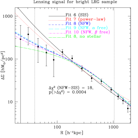
Next, we discuss the fits for the bright LRG sample, fits 6–10 in Table 3, with some fits shown with the real signal in Fig 9. The first fit we consider is the simple one-parameter fit (for $M$) with an assumed SIS profile and fixed stellar components, fit 6. The best-fit $\chi^{2}$ value of $28.6$ gives a $p$-value of 0.004, suggesting that this model is a poor fit to the data From Fig. 9, it is apparent that the SIS model once again overpredicts the signal for $40$–$100$ $h^{-1}$kpc scales.

Fit 7 is for a single power-law profile, with the exponent allowed to vary from the SIS value. As for the faint LRGs, the best-fit exponent is $-1.85\pm 0.05$, with a large decrease in best-fit $\chi^{2}$ of $11.9$ relative to fit 6, and a $p(>\Delta\chi^{2})=0.006$, so the general power-law profile is a markedly improved fit over the SIS. Fig. 9 indicates that (as for the faint LRG sample) this is the case primarily because this model predicts a lower signal than for the SIS model on $40$–$100$ $h^{-1}$kpc scales, at the expense of overpredicting the signal on $1$–$2$ $h^{-1}$Mpc scales.

Fit 8 is for $c$ and $M$ with fixed NFW $\alpha$, $\beta$, and stellar components. The best-fit $\chi^{2}$ is smaller than that of the SIS model (fit 6) by $18$, and therefore the NFW model is favored. The SIS model in fit 6 is ruled out relative to the NFW model at the 99.96 per cent CL, and the power-law model (fit 7) relative to the NFW at the 94 per cent CL. As shown in Fig. 9, the NFW model does a better job predicting the signal on $40$–$100$ $h^{-1}$kpc and $1$–$2$ $h^{-1}$Mpc scales than either of these other two models. This fit suggests a mass of $6.7\pm 0.8\times 10^{13}h^{-1}M_{\odot}$, so once again smaller than the predicted mean and median mass of this sample from the high normalization model halo mass function in Table 1 and closer to the lower limit, or to the predicted mean and median halo mass using the lower $\sigma_{8}$ cosmology.

For the concentration parameter in the NFW profile, we find $c=5.6\pm 0.6\mbox{(stat)}\pm 1\mbox{(sys)}$ once we apply the 20 per cent upward correction. This should be compared to a predicted $c=6.7$ in the high normalization model and $c=5.5$ in low normalization model. While the high normalization model predicts somewhat too high values, although within the errors, the low normalization model agrees well with the observations.

In fit 9, we constrain the concentration to the predicted value for this mass of $6.7$, but allow $\alpha$ to vary. As shown, the best-fit value is somewhat shallower than the assumed value of $-1.0$, at roughly the $3\sigma$ level. However, the $\chi^{2}$ value for this fit is worse than for fit 8 by roughly $1.4$, so the lower value of concentration is needed to match the signal (but the difference between the two values of concentration is not statistically significant).

In fit 10, we constrain the concentration to the predicted value of $6.7$, but allow $\beta$ to vary from canonical NFW value. As shown, the best-fit value of $2.7\pm 0.1$ is roughly $3\sigma$ from the canonical value, and the $\chi^{2}$ value of $9.4$ is actually slightly better than fit 18 which has $\beta$ fixed to its canonical value and $c$ free. This difference in $\chi^{2}$ (of $1.1$) is not actually statistically significant, however. As for the faint LRG sample, we lack the power to simultaneously contrain concentration along with either the inner or outer slopes.

For this sample, we also tried fitting simultaneously for $c$, NFW mass, and $M_{stellar}$. As for the faint LRG sample, the best-fit mass was very close to the assumed value, but with very large errors, so we lack the power to constrain this parameter. Also as before, we note that the distinctions between the three NFW models shown on Fig. 9 is very small compared to the difference between the SIS, power-law, and NFW models.

4.4.3 Mass to light relation

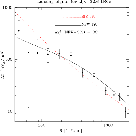
In this section we also include the results of an attempt to determine the relationship between LRG $r$-band luminosity and mass with finer binning in luminosity. The bright bin has been split into two bins at $M_{r}=-22.6$. In this way, we are able to split this sample, which has an average mass corresponding to massive groups, into one sample with groups and the other with clusters. Results for the masses and concentrations as a function of luminosity appear in Table 4, and signal for the brightest bin is shown in Fig. 10. As shown by this figure, even considering the small size of this lens sample, we still have significant ability to constrain the profile and differentiate between NFW and SIS due to the high halo mass. When we split the sample further, however, our ability to determine the profile to high precision degenerates, so we show no higher luminosity bins beyond this.

Concentrations have, as in the previous section, been adjusted upwards by 20 per cent. Masses have not been adjusted to account for scatter in the mass-luminosity relationship, because the degree of adjustment that is necessary is not yet clear. In general, however, this adjustment would have to lead to an increase of the best-fit masses, and hence it is clear that the mass is increasing quite rapidly with luminosity (roughly $M\propto L^{2}$). Thus, the luminosity of the central galaxy can be used as a rough measure of the cluster mass, at least for masses below $2\times 10^{14}M_{\odot}$, although the (possibly significant) scatter in this relation cannot be established by our statistical approach. This approach to finding clusters is much simpler than other methods, such as the number of red galaxies (i.e. richness) or integrated light within a certain window in real and redshift space.

Figure 10: Lensing signal for the $M_{r}<-22.6$ lens sample averaged over source sample.

Table 4: Masses and concentrations as a function of luminosity with finer binning in luminosity.

$M_{r}$ limits	$\langle L/L_{\odot}\rangle$	$M_{nfw,fit}$	$c_{nfw}$
	[$h^{-2}10^{10}$]	[$10^{13}h^{-1}M_{\odot}$]
$M_{r}>-22.3$	$5.2$	$2.9\pm 0.4$	$5.0\pm 0.6\mbox{(stat)}\pm 1\mbox{(sys)}$
$[-22.6,-22.3]$	$7.6$	$4.4\pm 0.7$	$6.8\pm 1.1\mbox{(stat)}\pm 1\mbox{(sys)}$
$M_{r}\leq-22.6$	$11.0$	$12.9\pm 1.9$	$5.0\pm 0.7\mbox{(stat)}\pm 1\mbox{(sys)}$

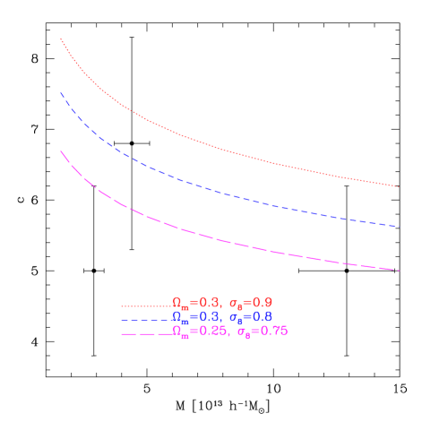
Fig. 11 shows the measured $c$ as a function of halo mass, along with the predictions for several cosmological models; as shown, somewhat lower normalizations are preferred. We postpone the comparison between the measured and predicted abundances to a future publication, since more work will be necessary to understand the effects of scatter in the $M(L)$ relationship on the measured NFW masses.

Figure 11: Measured NFW concentrations with statistical and systematic errors added in quadratures, shown as a function of best-fit NFW mass. The lines shown on the plot are predictions for several different cosmologies.

5 Interpretation and Conclusions

While our fits only use scales above 40 $h^{-1}$kpc due to concerns about lensing systematics, Figs. 8 and 9 include scales down to 20 $h^{-1}$kpc  the minimum scale probed. As shown in Fig. 8, the signal below 40 $h^{-1}$kpc is fit somewhat better by the single power-law models than by the NFW profile for the faint LRG sample, but this difference is not statistically significant, and can also be explained by an underestimation of stellar mass rather than by any problem with the NFW profile. Fig. 9 shows that the NFW model does a satisfactory job describing the data even below 40 $h^{-1}$kpc for the brighter lenses. For the faint lenses, several changes in parameters could raise the signal on scales below 40 $h^{-1}$kpc, such as an increase in stellar mass or a steeper inner slope for the DM profile. In both figures, we show the signal for the NFW fit without stellar component, and it is clear that the inclusion of the stellar component improves the agreement between model and observation below 50 $h^{-1}$kpc scales.

One might conclude, from Figs. 8 and 9, that it would be difficult to distinguish between inner DM profiles with any technique. However, there are several reasons why this is not the case. First, in using the lensing signal to distinguish between these density profiles, we are necessarily susceptible to some parameter degeneracies that are not a problem for other methods, such as those against which we compare below. Second, other methods have a different dynamic range; in particular both strong lensing and kinematic studies can probe to far smaller scales ($<10$ $h^{-1}$kpc). When combined with methods such as weak lensing that can constrain the profile on larger scales, in conjunction with constraints on the stellar profile, it seems conceivable that tight constraints could be placed on the inner dark matter profile.

We note that the fact that the models are either comparable with or larger than the lensing signal on $1$–$2$ $h^{-1}$Mpc scales implies that we have successfully extracted a sample of LRGs that resides almost exclusively in host halos rather than as satellites sitting at outskirts of clusters for which the signal would be reduced.

There are a number of conclusions that we can draw from these fit results. First, the division into stellar and halo components allows us to fit the data very well. Adiabatic contraction does not seem to be necessary for our description on the scales of interest ($R>40$ $h^{-1}$kpc) because of the relatively low stellar to halo mass ratio, but the addition of the stellar component improves the fit on small scales over the simple NFW profile and there is some evidence that it may even be underestimated for the faint sample. We note that it is possible that AC occurred at a significantly earlier stage in the galaxy’s formation, when $M_{stellar}/M_{halo}$ was much larger. In that case, more significant AC on larger scales would have caused a steepening of the profile, which would then approximately be preserved through its later mergers (Boylan-Kolchin et al., 2005; Kazantzidis et al., 2006). This is another possible explanation for the excess over the NFW plus stellar mass model on $20<R<40$ $h^{-1}$kpc scales; however, due to the uncertain systematics in this regime, we do not attempt to place constraints directly. Furthermore, we are unable to constrain the form of the stellar component; on the scales under consideration, a point mass works nearly as well as a Hernquist profile.

We compare these results with those from other methods that are used to determine the density profiles. Recent X-ray studies have found that the profile is consistent with the NFW model (Vikhlinin et al., 2005; Fukazawa et al., 2006; Humphrey et al., 2006), though with indications for poor groups (consistent in mass with our “faint” sample) of some excess over NFW on small scales (Vikhlinin et al., 2005), similar to our finding that the data is above the NFW model with stellar component in Fig. 8 for the fainter LRG sample. Thus, our results seem to be consistent with those from X-ray studies.

Some kinematic and strong lensing studies (e.g., Rusin & Ma 2001, Koopmans & Treu 2003, Huterer & Ma 2004, Koopmans et al. 2006) have suggested a logarithmic slope $\sim-2$ on scales below $10$ kpc, where optical observations provide velocity dispersion information and strong lensing occurs. It is entirely possible that in that regime adiabatic contraction actually is necessary to understand the profile, and leads to the steepening of the profile compared to NFW. It is also possible that due to selection effects in the strong-lensing samples, they are not entirely comparable to our LRG-selected sample of groups and clusters. We note that we have central velocity dispersions for the LRG sample used in this analysis, which has been used to learn about AC and dark matter inside the optical radius (Padmanabhan et al., 2004). In the future it would be interesting to combine the weak lensing information with the kinematic information to learn more about the mass profile in the inner parts of the clusters.

Studies of galaxy kinematics on larger scales, out to several Mpc, have found a strong preference for the NFW profile over a SIS profile on the same scales as this study. These works (e.g., van der Marel et al. 2000; Biviano & Girardi 2003; Rines et al. 2003; Rines & Diaferio 2006) typically focus on several tens of clusters with a large number of spectroscopic redshifts per cluster, and determine the profile using the cluster infall patterns. Generally the clusters for which this technique is used are in a higher mass range than those considered here, $10^{14}$ - $10^{15}h^{-1}M_{\odot}$. It is useful to know that our results, which focus on the average profile of groups and clusters in a lower mass range, have been found to be true for individual higher mass clusters as well.

We can see from the fits to the two samples separately that a characteristic halo mass for LRGs overall is $\sim 5\times 10^{13}h^{-1}M_{\odot}$. This corresponds to the transition regime between groups and low mass clusters. This is not too surprising, since the comoving number density of these objects ($1.2\times 10^{-4}(h/\mbox{Mpc})^{3}$) is an order of magnitude larger than for large clusters, and hence the typical LRG halo mass must be significantly smaller than that of massive clusters. If we adopt the definition that clusters have virial masses above $10^{14}M_{\odot}$ then, given that the best fit mass of our bright sample corresponds to this value when we use $h=0.7$, half of the halos in the bright sample can be defined as low mass clusters. This is also consistent with the findings in Loh & Strauss (2006, in prep.) that the typical LRG resides in groups, with some in the field, and some fraction in large clusters. We find that on average, brighter central LRGs reside in more massive halos, and the relation scales as $M\propto L^{2}$ over the range we observe.

When fitting to 2 $h^{-1}$Mpc, a profile that has a change in logarithmic slope with scale seems to provide the best fit to the data; the SIS profile is ruled out more robustly than a general power-law profile. Specifically, for the faint LRG sample, the SIS is ruled out relative to the NFW profile at the 96 per cent CL; for the bright LRG sample, the SIS is ruled out relative to NFW at the 99.96 per cent CL.

Use of the the canonical slopes $\alpha=-1$ and $\beta=3$ gives best-fit concentrations of $5.0\pm 0.6\pm 1$ and $5.6\pm 0.5\pm 1$ for faint and bright lens samples, respectively, where the first error is statistical and second systematic, since the scatter in concentration-mass relation leads to a bias in the fits and we do not have sufficiently large simulated samples of groups and clusters to model this bias accurately. By splitting the brighter bin further, we are able to obtain two different concentration measurements for group and cluster-sized halos individually, as discussed in §4.4.3. The results are lower than the expected values from high normalization $\Lambda$CDM simulation, as shown in Fig. 11. If we allow $\Omega_{m}=0.25$ and $\sigma_{8}=0.75$ in accordance with the recent WMAP 3-year results (Spergel et al., 2006), the predicted values of $c$ are low enough that the discrepancies are reduced to an acceptable level (below $1\sigma$ when both statistical and systematic errors are included). Note that in principle, the statistical errors are sufficiently small that the method can provide constraining power to differentiate among currently viable cosmological models. We refrain from making strong cosmological implications from this comparison because the method has not been calibrated yet in simulations over this halo mass range. When applied to lower masses below $10^{13}M_{\odot}$ it was found that the method underestimates the true concentration parameter by about 20 per cent (Mandelbaum et al., 2005b), a correction we have applied in the present analysis as well.

In general, therefore, our results are in accordance with the predictions of $\Lambda$CDM N-body simulation predictions of halo profiles and statistically the measurements have very high signal to noise. More detailed analysis in the future will be able to differentiate among the cosmological models using both the measured cluster profiles and the abundance information.

Appendix A Effects of non-weak shear on shear estimator

Here we compute the relation between the mean ellipticity and the distortion matrix. This relation has previously been examined by Schneider & Seitz (1995) for the case with $\omega=0$; they derived an equation that is essentially equivalent to our Eq. (38), although they did not provide the Taylor expansion in $g$. The analysis in this paper only makes use of the terms through second order in the weak lensing approximation (i.e. second order in $\kappa$ or in $\Sigma_{c}^{-1}$) since this is adequate for the LRGs at tens of kpc radii where $\kappa\sim 0.1$. We do however present the full formalism here, including all orders in $\Sigma_{c}^{-1}$, in the hope that it will be useful in the future.

The analysis here makes extensive use of the fact that our ellipticities transform covariantly under shear (this is in fact true for all the adaptive ellipticities, e.g. as considered by Bernstein & Jarvis 2002); note that many of the other ellipticities used in the literature, such as “KSB” ellipticities (Kaiser et al., 1995), do not share this property and the results of this section do not apply to them.

The local relation between the source and image planes is usually described by the Jacobian:

$${\textbf{{J}}}=\frac{\partial{\mn@boldsymbol{x}}_{S}}{\partial{\mn@boldsymbol{x}}_{I}}=\left(\begin{array}[]{cc}1-\gamma_{+}-\kappa&-\gamma_{\times}+\omega\\ -\gamma_{\times}-\omega&1+\gamma_{+}-\kappa\end{array}\right),$$ (32)

where the rows indicate the $1$ and $2$ components of ${\mn@boldsymbol{x}}_{S}$ and the columns indicate those of ${\mn@boldsymbol{x}}_{I}$. Our basic problem here is to relate the mean ellipticity of the galaxies, $\langle{\mn@boldsymbol{e}}\rangle$, to the entries in J. In particular, we will find that $\langle{\mn@boldsymbol{e}}\rangle$ is not simply proportional to $\mn@boldsymbol{\gamma}$.

It is most convenient here to work with the singular-value decomposition of J rather than with J itself. The singular-value decomposition is $\textbf{{J}}=\textbf{{R}}(\varphi)\textbf{{D}}\textbf{{R}}(\theta)$, where D is diagonal and $\textbf{{R}}(\alpha)$ represents a counterclockwise rotation by angle $\alpha$. If we define ${\cal A}={\rm Tr}\,\textbf{{D}}/2$, then this can be written as

$$\textbf{{J}}={\cal A}\textbf{{R}}(\varphi)\ \left(\begin{array}[]{cc}1-g&0\\ 0&1+g\end{array}\right)\textbf{{R}}(\theta)\equiv{\cal A}\textbf{{R}}(\varphi)\textbf{{T}}(\delta)\textbf{{R}}(\theta).$$ (33)

The four variables $\{\gamma_{+},\gamma_{\times},\kappa,\omega\}$ in the Jacobian have thus been replaced with the four variables $\{g,\theta,{\cal A},\varphi\}$. The explicit formula for the conversion can be derived from the rectangular-to-polar conversion, Eq. (A5) of Hirata & Seljak (2003), which gives:

$$2(1-\kappa) = 2{\cal A}\cos(\varphi+\theta),$$

$$-2\omega = 2{\cal A}\sin(\varphi+\theta),$$

$$-2\gamma_{+} = -2g\cos(\varphi-\theta),{\rm~{}and}$$

$$-2\gamma_{\times} = -2g\sin(\varphi-\theta).$$ (34)

The solution to this system of equations is

$${\cal A} = \sqrt{(1-\kappa)^{2}+\omega^{2}},$$

$$g = \sqrt{\frac{\gamma_{+}^{2}+\gamma_{\times}^{2}}{(1-\kappa)^{2}+\omega^{2}}},$$

$$\varphi = \frac{1}{2}\left(-\arctan\frac{\omega}{1-\kappa}+\arctan\frac{\gamma_{\times}}{\gamma_{+}}\right),{\rm~{}and}$$

$$\theta = \frac{1}{2}\left(-\arctan\frac{\omega}{1-\kappa}-\arctan\frac{\gamma_{\times}}{\gamma_{+}}\right).$$ (35)

The arguments of $\arctan$ in the last two lines have been written such that the numerator and denominator give the correct quadrant for the arctangent. Note that for the case of a single-screen lens with $\omega=0$, $g$ reduces to the familiar “reduced shear” $g=\gamma/(1-\kappa)$ (Schneider & Seitz, 1995).

Of these four variables, ${\cal A}$ re-scales the source plane and so has no effect on the ellipticities. The rotation $\textbf{{R}}(\varphi)$ rotates the source plane and for randomly oriented source galaxies can have no effect on the average ellipticity. The transformation $\textbf{{T}}(g)$ in Eq. (33) can produce net ellipticity in the $+$ direction; and $\textbf{{R}}(\theta)$ rotates the image plane by angle $\theta$ and hence $\langle\mn@boldsymbol{e}\rangle$ by angle $2\theta$. Thus the observable $\langle\mn@boldsymbol{e}\rangle$ depends only on $g$ and $\theta$, and moreover the dependence on $\theta$ corresponds trivially to a rotation.

Our problem is thus reduced to determining $\langle\mn@boldsymbol{e}\rangle$ for the special case where $\textbf{{J}}=\textbf{{T}}(g)$. In this case symmetry considerations imply $\langle e_{\times}\rangle=0$, so we need only determine $\langle e_{+}\rangle$. If the intrinsic ellipticity of a galaxy is $\mn@boldsymbol{e^{(0)}}$, then the equation for the final ellipticity is given by Eq. (2.5) of Miralda-Escude (1991):

$$e_{+}=\frac{e^{(0)}_{+}+\delta}{1+\delta e^{(0)}_{+}},$$ (36)

where the distortion $\delta$ is related to $g$ by Eqs. (2-7) and (2-8) of Bernstein & Jarvis (2002):

$$\delta=\tanh(2\,{\rm arctanh}\,g)=\frac{2g}{1+g^{2}}.$$ (37)

It is simplest to evaluate $\langle e_{+}\rangle$ for a population of sources whose intrinsic ellipticities have fixed magnitude $e^{(0)}$ and random orientation $\phi$; other source populations can be handled by further averaging over the appropriate distribution for $e^{(0)}$. In this case, we may write $e^{(0)}_{+}=e^{(0)}\cos 2\phi$, so that

$$\langle e_{+}\rangle = \frac{1}{2\pi}\int_{0}^{2\pi}\frac{e^{(0)}\cos 2\phi+\delta}{1+\delta e^{(0)}\cos 2\phi}\,{\rm d}\phi$$ (38)

$$= \frac{1}{2\pi}\int_{0}^{2\pi}\left(\delta^{-1}+\frac{\delta-\delta^{-1}}{1+\delta e^{(0)}\cos 2\phi}\right)\,{\rm d}\phi$$

$$= \delta^{-1}+\frac{\delta-\delta^{-1}}{\sqrt{1-\delta^{2}e^{(0)\,2}}}.$$

(The first term in the second line is integrated trivially, while the second term can be reduced to a rational integral by the substitution $z=\tan\phi$.) We are interested in the weak-shear regime where we can use the Taylor expansion in $\delta$, which is easily obtained from the binomial expansion of $(1-\delta^{2}e^{(0)\,2})^{-1/2}$:

$$\langle e_{+}\rangle = \left(1-\frac{1}{2}e^{(0)\,2}\right)\delta+\left(\frac{1}{2}e^{(0)\,2}-\frac{3}{8}e^{(0)\,4}\right)\delta^{3}$$ (39)

$$+\left(\frac{3}{8}e^{(0)\,4}-\frac{5}{16}e^{(0)\,6}\right)\delta^{5}$$

$$+\left(\frac{5}{16}e^{(0)\,6}-\frac{35}{128}e^{(0)\,8}\right)\delta^{7}+...\;.$$

(There is no singularity at $\delta=0$ because the coefficients of $\delta^{-1}$ cancel.) In the weak lensing literature, $g$ is usually used instead of $\delta$; substitution of Eq. (37) into Eq. (39) yields

$$\langle e_{+}\rangle=\sum_{n=0}^{\infty}\zeta_{n}g^{2n+1},$$ (40)

where the first few coefficients in the expansion are

$$\zeta_{0} = 2-e^{(0)\,2},$$

$$\zeta_{1} = -2+5e^{(0)\,2}-3e^{(0)\,4},$$

$$\zeta_{2} = 2-13e^{(0)\,2}+21e^{(0)\,4}-10e^{(0)\,6},{\rm~{}and}$$

$$\zeta_{3} = -2+25e^{(0)\,2}-78e^{(0)\,4}+90e^{(0)\,6}-35e^{(0)\,8}.$$ (41)

For an ensemble of source galaxies with different intrinsic ellipticities, the values $e^{(0)\,n}$ should be replaced by the appropriate moments $\langle e^{(0)\,n}\rangle$ of the source galaxy distribution.

In the case of a single-screen lens, it is convenient to expand $\langle e_{+}\rangle$ in powers of the lensing strength $\Sigma_{c}^{-1}$, since both $\gamma$ and $\kappa$ are proportional to this quantity. In particular, we have

$$\gamma_{+}=\Delta\Sigma_{+}\,\Sigma_{c}^{-1},\quad\gamma_{\times}=\Delta\Sigma_{\times}\,\Sigma_{c}^{-1},{\rm~{}and~{}}\kappa=\Sigma\,\Sigma_{c}^{-1}.$$ (42)

Here $\Sigma$ is the surface density at the location of the image and $\Delta\mn@boldsymbol{\Sigma}$ is the surface density contrast defined in Fourier space by

$$\Delta\Sigma_{+}(\mn@boldsymbol{l})\pm{\rm i}\Delta\Sigma_{\times}(\mn@boldsymbol{l})={\rm e}^{\pm 2{\rm i}\arctan(l_{2}/l_{1})}\Sigma(\mn@boldsymbol{l}).$$ (43)

In the coordinate system where $\Delta\mn@boldsymbol{\Sigma}$ is in the $+$ direction, Eq. (40) then becomes

$$\langle e_{+}\rangle=\sum_{n=0}^{\infty}\zeta_{n}\left(\frac{|\Delta\mn@boldsymbol{\Sigma}|\,\Sigma_{c}^{-1}}{1-\Sigma\,\Sigma_{c}^{-1}}\right)^{2n+1}.$$ (44)

This is turned into a power series in $\Sigma_{c}^{-1}$ using the binomial theorem for negative powers,

$$(1-x)^{-(2n+1)}=\sum_{j=0}^{\infty}\left(\!\!\begin{array}[]{c}2n+j\\ 2n\end{array}\!\!\right)x^{j},$$ (45)

which gives:

$$\langle e_{+}\rangle=\sum_{n=0}^{\infty}\zeta_{n}|\Delta\mn@boldsymbol{\Sigma}|^{2n+1}\Sigma_{c}^{-(2n+1)}\sum_{j=0}^{\infty}\left(\!\!\begin{array}[]{c}2n+j\\ 2n\end{array}\!\!\right)\Sigma^{j}\Sigma_{c}^{-j}.$$ (46)

We now consolidate terms with the same exponent by defining $k=2n+j+1$:

$$\langle e_{+}\rangle = \sum_{k=1}^{\infty}\left[\sum_{n=0}^{\lfloor(k-1)/2\rfloor}\left(\!\!\begin{array}[]{c}2n+j\\ 2n\end{array}\!\!\right)\zeta_{n}|\Delta\mn@boldsymbol{\Sigma}|^{2n+1}\Sigma^{k-2n-1}\right]$$ (50)

$$\times\Sigma_{c}^{-k}.$$

For the purposes of this work, we only use the $k=1$ term in Eq. 50 (or equivalently, the $n=0$ term in Eq. 44), since higher order terms are 3rd-order or higher in $\kappa$ and $\gamma$. This lowest order term gives

$$\langle e_{+}\rangle=(2-e^{(0)2})\frac{|\Delta\mn@boldsymbol{\Sigma}|\,\Sigma_{c}^{-1}}{1-\Sigma\,\Sigma_{c}^{-1}}$$ (51)

we identify the $(2-e^{(0)2})$ factor with $2{\cal R}$, twice the shear responsivity. We then do the lowest order Taylor expansion of this equation, which tells us that

$$\langle e_{+}\rangle=2{\cal R}\langle\Delta\Sigma\,\Sigma_{c}^{-1}+\Delta\Sigma\,\Sigma\,\Sigma_{c}^{-2}\rangle$$ (52)

When we do the usual approximation that the lenses are statistically identical, which is reasonable for these volume-limited samples, then the correction due to non-weak shear is

$$\langle e_{+}\rangle=2{\cal R}\langle\Delta\Sigma\rangle\langle\Sigma_{c}^{-1}\rangle\left(1+\frac{\langle\Delta\Sigma\,\Sigma\rangle}{\langle\Delta\Sigma\rangle}\frac{\langle\Sigma_{c}^{-2}\rangle}{\Sigma_{c}^{-1}}\right)$$ (53)

Note that the factor in parenthesis is not the same as $1+\kappa$, for two reasons. First, $\langle\Delta\Sigma\,\Sigma\rangle/\langle\Delta\Sigma\rangle>\langle\Sigma\rangle$ since the massive objects get weighted more heavily. Second, $\langle\Sigma_{c}^{-2}\rangle/\langle\Sigma_{c}^{-1}\rangle>\langle\Sigma_{c}^{-1}\rangle$. Both of these issues will tend to make reduced shear more important than the naive argument in the text that it depends on the size of $1+\kappa$.

References

- Abazajian et al. (2003) Abazajian K. et al., 2003, AJ, 126, 2081
- Abazajian et al. (2004) Abazajian K. et al., 2004, AJ, 128, 502
- Abazajian et al. (2005) Abazajian K. et al., 2005, AJ, 129, 1755
- Adelman-McCarthy et al. (2006) Adelman-McCarthy J. K. et al., 2006, ApJS, 162, 38
- Agustsson & Brainerd (2005) Agustsson I., Brainerd T. G., 2005, preprint (astro-ph/0509405)
- Albert et al. (1977) Albert C. E., White R. A., Morgan W. W., 1977, ApJ, 211, 309
- Allen (1998) Allen S. W., 1998, MNRAS, 296, 392
- Arabadjis et al. (2002) Arabadjis J. S., Bautz M. W., Garmire G. P., 2002, ApJ, 572, 66
- Athreya et al. (2002) Athreya R. M., Mellier Y., van Waerbeke L., Pelló R., Fort B., Dantel-Fort M., 2002, A&A, 384, 743
- Avila-Reese et al. (1999) Avila-Reese V., Firmani C., Klypin A., Kravtsov A. V., 1999, MNRAS, 310, 527
- Azzaro et al. (2006) Azzaro M., Patiri S. G., Prada F., Zentner A. R., 2006, preprint (astro-ph/0607139)
- Baldry et al. (2004) Baldry I. K., Glazebrook K., Brinkmann J., Ivezić Ž., Lupton R. H., Nichol R. C., Szalay A. S., 2004, ApJ, 600, 681
- Bell et al. (2004) Bell E. F. et al., 2004, ApJ, 608, 752
- Bernardi et al. (2003) Bernardi M. et al., 2003, AJ, 125, 1866
- Bernstein & Jarvis (2002) Bernstein G. M., Jarvis M., 2002, AJ, 123, 583
- Bernstein & Norberg (2002) Bernstein G. M., Norberg P., 2002, AJ, 124, 733
- Biviano & Girardi (2003) Biviano A., Girardi M., 2003, ApJ, 585, 205
- Blanton et al. (2003a) Blanton M. R., Lin H., Lupton R. H., Maley F. M., Young N., Zehavi I., Loveday J., 2003a, AJ, 125, 2276
- Blanton et al. (2003b) Blanton M. R. et al., 2003b, AJ, 125, 2348
- Blanton et al. (2003c) Blanton M. R. et al., 2003c, ApJ, 592, 819
- Blanton et al. (2005) Blanton M. R. et al., 2005, AJ, 129, 2562
- Blumenthal et al. (1986) Blumenthal G. R., Faber S. M., Flores R., Primack J. R., 1986, ApJ, 301, 27
- Bower et al. (1992) Bower R. G., Lucey J. R., Ellis R. S., 1992, MNRAS, 254, 601
- Boylan-Kolchin et al. (2005) Boylan-Kolchin M., Ma C.-P., Quataert E., 2005, MNRAS, 362, 184
- Bruzual & Charlot (2003) Bruzual G., Charlot S., 2003, MNRAS, 344, 1000
- Bullock et al. (2001) Bullock J. S., Kolatt T. S., Sigad Y., Somerville R. S., Kravtsov A. V., Klypin A. A., Primack J. R., Dekel A., 2001, MNRAS, 321, 559
- Clowe et al. (2000) Clowe D., Luppino G. A., Kaiser N., Gioia I. M., 2000, ApJ, 539, 540
- Clowe & Schneider (2001) Clowe D., Schneider P., 2001, A&A, 379, 384
- Coil et al. (2004) Coil A. L. et al., 2004, ApJ, 609, 525
- Cool et al. (2006) Cool R. J., Eisenstein D. J., Johnston D., Scranton R., Brinkmann J., Schneider D. P., Zehavi I., 2006, AJ, 131, 736
- Davis et al. (2003) Davis M. et al., 2003, in Proceedings of the SPIE, 4834, 161
- Davis et al. (2005) Davis M., Gerke B. F., Newman J. A., 2005, ASP Conf. Ser. 339, 128
- de Zeeuw et al. (2002) de Zeeuw P. T. et al., 2002, MNRAS, 329, 513
- Diemand et al. (2005) Diemand J., Zemp M., Moore B., Stadel J., Carollo M., 2005, MNRAS, 364, 665
- Djorgovski & Davis (1987) Djorgovski S., Davis M., 1987, ApJ, 313, 59
- Donoso et al. (2006) Donoso E., O’Mill A. L., Lambas D. G., 2006, preprint (astro-ph/0603471)
- Eisenstein et al. (2001) Eisenstein D. J. et al., 2001, AJ, 122, 2267
- Eisenstein et al. (2003) Eisenstein D. J. et al., 2003, ApJ, 585, 694
- Eisenstein et al. (2005a) Eisenstein D. J., Blanton M., Zehavi I., Bahcall N., Brinkmann J., Loveday J., Meiksin A., Schneider D., 2005a, ApJ, 619, 178
- Eisenstein et al. (2005b) Eisenstein D. J. et al., 2005b, ApJ, 633, 560
- Eke et al. (2001) Eke V. R., Navarro J. F., Steinmetz M., 2001, ApJ, 554, 114
- Faber (1973) Faber S. M., 1973, ApJ, 179, 731
- Faber & Jackson (1976) Faber S. M., Jackson R. E., 1976, ApJ, 204, 668
- Ferreras et al. (2005) Ferreras I., Saha P., Williams L. L. R., 2005, ApJL, 623, L5
- Finkbeiner et al. (2004) Finkbeiner D. P. et al., 2004, AJ, 128, 2577
- Fukazawa et al. (2006) Fukazawa Y., Botoya-Nonesa J. G., Pu J., Ohto A., Kawano N., 2006, ApJ, 636, 698
- Fukugita et al. (1996) Fukugita M., Ichikawa T., Gunn J. E., Doi M., Shimasaku K., Schneider D. P., 1996, AJ, 111, 1748
- Fukugita et al. (1998) Fukugita M., Hogan C. J., Peebles P. J. E., 1998, ApJ, 503, 518
- Fukushige & Makino (1997) Fukushige T., Makino J., 1997, ApJL, 477, L9+
- Fukushige & Makino (2001) Fukushige T., Makino J., 2001, ApJ, 557, 533
- Fukushige & Makino (2003) Fukushige T., Makino J., 2003, ApJ, 588, 674
- Ghigna et al. (2000) Ghigna S., Moore B., Governato F., Lake G., Quinn T., Stadel J., 2000, ApJ, 544, 616
- Gnedin et al. (2004) Gnedin O. Y., Kravtsov A. V., Klypin A. A., Nagai D., 2004, ApJ, 616, 16
- Gnedin (2005) Gnedin O. Y., 2005, preprint (astro-ph/0510549)
- Gunn et al. (2006) Gunn J. E. et al., 2006, AJ, 131, 2332
- Gunn et al. (1998) Gunn J. E. et al., 1998, AJ, 116, 3040
- Hirata & Seljak (2003) Hirata C., Seljak U., 2003, MNRAS, 343, 459
- Hirata et al. (2004) Hirata C. M. et al., 2004, MNRAS, 353, 529
- Hoekstra et al. (2001) Hoekstra H. et al., 2001, ApJL, 548, L5
- Hoekstra et al. (2005) Hoekstra H., Hsieh B. C., Yee H. K. C., Lin H., Gladders M. D., 2005, ApJ, 635, 73
- Hogg et al. (2001) Hogg D. W., Finkbeiner D. P., Schlegel D. J., Gunn J. E., 2001, AJ, 122, 2129
- Hogg et al. (2002) Hogg D. W. et al., 2002, AJ, 124, 646
- Humphrey et al. (2006) Humphrey P. J., Buote D. A., Gastaldello F., Zappacosta L., Bullock J. S., Brighenti F., Mathews W. G., 2006, preprint (astro-ph/0601301)
- Huterer & Ma (2004) Huterer D., Ma C.-P., 2004, ApJL, 600, L7
- Ivezić et al. (2004) Ivezić Ž. et al., 2004, Astronomische Nachrichten, 325, 583
- Jing & Suto (2000) Jing Y. P., Suto Y., 2000, ApJL, 529, L69
- Kaiser et al. (1995) Kaiser N., Squires G., Broadhurst T., 1995, ApJ, 449, 460
- Kauffmann et al. (2003) Kauffmann G. et al., 2003, MNRAS, 341, 33
- Kazantzidis et al. (2006) Kazantzidis S., Zentner A. R., Kravtsov A. V., 2006, ApJ, 641, 647
- Klypin et al. (2001) Klypin A., Kravtsov A. V., Bullock J. S., Primack J. R., 2001, Apj, 554, 903
- Koopmans & Treu (2003) Koopmans L. V. E., Treu T., 2003, ApJ, 583, 606
- Koopmans et al. (2006) Koopmans L. V. E., Treu T., Bolton A. S., Burles S., Moustakas L. A., 2006, preprint (astro-ph/0601628)
- Kormendy & Djorgovski (1989) Kormendy J., Djorgovski S., 1989, ARA&A, 27, 235
- Kravtsov et al. (1997) Kravtsov A. V., Klypin A. A., Khokhlov A. M., 1997, ApJS, 111
- Kronawitter et al. (2000) Kronawitter A., Saglia R. P., Gerhard O., Bender R., 2000, A&AS, 144, 53
- Lee & Pen (2001) Lee J., Pen U., 2001, ApJ, 555, 106
- Lupton et al. (2001) Lupton R. H., Gunn J. E., Ivezić Z., Knapp G. R., Kent S., Yasuda N., 2001, in ASP Conf. Ser. 238, 269
- Madgwick et al. (2003) Madgwick D. S. et al., 2003, ApJ, 599, 997
- Mandelbaum et al. (2005a) Mandelbaum R. et al., 2005a, MNRAS, 361, 1287
- Mandelbaum et al. (2005b) Mandelbaum R., Tasitsiomi A., Seljak U., Kravtsov A. V., Wechsler R. H., 2005b, MNRAS, 362, 1451
- Mandelbaum et al. (2005c) Mandelbaum R., Hirata C. M., Broderick T., Seljak U., Brinkmann J., 2005c, preprint (astro-ph/0507108)
- Mandelbaum et al. (2005d) Mandelbaum R., Seljak U., Kauffmann G., Hirata C. M., Brinkmann J., 2005d, preprint (astro-ph/0511164)
- Mandelbaum et al. (2006) Mandelbaum R., Hirata C. M., Ishak M., Seljak U., Brinkmann J., 2006, MNRAS, 367, 611
- Masjedi et al. (2005) Masjedi M. et al., 2005, preprint (astro-ph/0512166)
- Miralda-Escude (1991) Miralda-Escude J., 1991, ApJ, 380, 1
- Moore et al. (1998) Moore B., Governato F., Quinn T., Stadel J., Lake G., 1998, ApJL, 499, L5
- Morgan et al. (1975) Morgan W. W., Kayser S., White R. A., 1975, ApJ, 199, 545
- Navarro et al. (1996) Navarro J. F., Frenk C. S., White S. D. M., 1996, ApJj, 462, 563
- Padmanabhan et al. (2004) Padmanabhan N. et al., 2004, New Astronomy, 9, 329
- Padmanabhan et al. (2005) Padmanabhan N. et al., 2005, MNRAS, 359, 237
- Parker et al. (2005) Parker L. C., Hudson M. J., Carlberg R. G., Hoekstra H., 2005, ApJ, 634, 806
- Pier et al. (2003) Pier J. R., Munn J. A., Hindsley R. B., Hennessy G. S., Kent S. M., Lupton R. H., Ivezić Ž., 2003, AJ, 125, 1559
- Ponman et al. (1994) Ponman T. J., Allan D. J., Jones L. R., Merrifield M., McHardy I. M., Lehto H. J., Luppino G. A., 1994, Nature, 369, 462
- Press & Schechter (1974) Press W. H., Schechter P., 1974, ApJ, 187, 425
- Read & Trentham (2005) Read J. I., Trentham N., 2005, preprint (astro-ph/0502517)
- Richards et al. (2003) Richards G. T. et al., 2002, AJ, 123, 2945
- Roberts & Haynes (1994) Roberts M. S., Haynes M. P., 1994, ARA&A, 32, 115
- Rines et al. (2003) Rines K., Geller M. J., Kurtz M. J., Diaferio A., 2003, AJ, 126, 2152
- Rines & Diaferio (2006) Rines K., Diaferio A., 2006, preprint (astro-ph/0602032)
- Rusin & Ma (2001) Rusin D., Ma C.-P., 2001, ApJL, 549, L33
- Schlegel et al. (1998) Schlegel D. J., Finkbeiner D. P., Davis M., 1998, ApJ, 500, 525
- Schneider & Seitz (1995) Schneider P., Seitz C., 1995, A&A, 294, 411
- Seljak (2000) Seljak U., 2000, MNRAS, 318, 203
- Seljak & Warren (2004) Seljak U., Warren M. S., 2004, MNRAS, 355, 129
- Sellwood & McGaugh (2005) Sellwood J. A., McGaugh S. S., 2005, ApJ, 634, 70
- Sheldon et al. (2001) Sheldon E. S. et al., 2001, ApJ, 554, 881
- Sheth & Tormen (1999) Sheth R. K., Tormen G., 1999, MNRAS, 308, 119
- Smith et al. (2002) Smith J. A. et al., 2002, AJ, 123, 2121
- Spergel et al. (2006) Spergel D. N. et al., 2006, preprint (astro-ph/0603449)
- Stoughton et al. (2002) Stoughton C. et al., 2002, AJ, 123, 485
- Strauss et al. (2002) Strauss M. A. et al., 2002, AJ, 124, 1810
- Tasitsiomi et al. (2004) Tasitsiomi A., Kravtsov A. V., Gottlöber S. an d Klypin A. A., 2004, ApJ, 607, 125
- Tucker et al. (2005) Tucker D. et al., 2005
- van der Marel et al. (2000) van der Marel R. P., Magorrian J., Carlberg R. G., Yee H. K. C., Ellingson E., 2000, AJ, 119, 2038
- Vikhlinin et al. (1999) Vikhlinin A., McNamara B. R., Hornstrup A., Quintana H., Forman W., Jones C., Way M., 1999, ApJL, 520, L1
- Vikhlinin et al. (2005) Vikhlinin A., Kravtsov A., Forman W., Jones C., Markevitch M., Murray S. S., Van Speybroeck L., 2005, preprint (astro-ph/0507092)
- Visvanathan & Sandage (1977) Visvanathan N., Sandage A., 1977, ApJ, 216, 214
- Wechsler et al. (2002) Wechsler R. H., Bullock J. S., Primack J. R., Kravtsov A. V., Dekel A., 2002, ApJ, 568, 52
- Yang et al. (2006) Yang X., van den Bosch F. C., Mo H. J., Mao S., Kang X., Weinmann S. M., Guo Y., Jing Y. P., 2006, MNRAS, 369, 1293
- York, et al. (2000) York D. G. et al., 2000, AJ, 120, 1579
- Zehavi et al. (2005) Zehavi I. et al., 2005, ApJ, 621, 22
- Zhao et al. (2003) Zhao D. H., Jing Y. P., Mo H. J., Börner G., 2003, ApJL, 597, L9