The Spitzer c2d Survey of Nearby Dense Cores: III: Low Mass Star Formation in a Small Group, L1251B

Abstract

We present a comprehensive study of a low-mass star-forming region, L1251B, at wavelengths from the near-infrared to the millimeter. L1251B, where only one protostar, IRAS 22376+7455, was known previously, is confirmed to be a small group of protostars based on observations with the Spitzer Space Telescope. The most luminous source of L1251B is located 5$\arcsec$ north of the IRAS position. A near-infrared bipolar nebula, which is not associated with the brightest object and is located at the southeast corner of L1251B, has been detected in the IRAC bands. OVRO and SMA interferometric observations indicate that the brightest source and the bipolar nebula source in the IRAC bands are deeply embedded disk sources. Submillimeter continuum observations with single-dish telescopes and the SMA interferometric observations suggest two possible prestellar objects with very high column densities. Outside of the small group, many young stellar object candidates have been detected over a larger region of $12\arcmin\times 12\arcmin$. Extended emission to the east of L1251B has been detected at 850 µm; this “east core” may be a site for future star formation since no point source has been detected with IRAC or MIPS. This region is therefore a possible example of low-mass cluster formation, where a small group of pre- and protostellar objects (L1251B) is currently forming, alongside a large starless core (the east core).

1 INTRODUCTION

Stars form out of dense cores of molecular gas, but the details of this process are far from understood. To probe this process, continuum and line data of star-forming regions can be combined to provide a coherent, self-consistent picture of young stellar objects and their associated, gaseous environments, i.e., densities, temperatures, and velocities. Indeed, these physical properties are intertwined within dynamical and luminosity evolution during star formation. Observations over a wide range of continuum wavelengths can test models of dynamical and luminosity evolution because different parts of a star-forming region are traced by different wavelengths. For example, cold envelopes are traced by (sub)millimeter dust emission which yield information on total (gas+dust) masses. On the other hand, inner envelopes or disks are traced by infrared emission, which is directly related to internal luminosity sources. In addition, observations of a wide variety of lines yield information about associated gas motions and can probe the excitation conditions along various lines of sight in star-forming regions. Chemistry is also important to understand, however. For example, velocity structures derived from molecular spectra can be misinterpreted if incongruous abundance profiles are adopted. Several studies have shown that chemical evolution is not independent of dynamical and luminosity evolution (Rawlings & Yates 2001; Doty et al. 2002; Lee, Bergin & Evans 2004).

Most star formation in the Galaxy occurs in clusters embedded within giant molecular clouds (Lada & Lada 2003), but the high surface densities of young stellar objects make it difficult to disentangle the star formation process. Although not considered “typical” star formation, more isolated cases have been examined vigorously since they are much less complicated and observations of them are easier to interpret (Di Francesco et al. 2006). Between these extremes lie the smaller groups of young stellar objects (i.e., $N$ $<$ 10), which may have condensed out of a single dense core (Machida et al. 2005). Examining such groups in detail may provide access to understanding features of the clustered star formation process, yet are relatively uncomplicated and hence easier to understand. Indeed, our Galactic neighborhood is resplendent in examples of groups of young stellar objects (YSOs), whose associated continuum and line emission can be examined to probe how they formed.

In this paper, we examine continuum emission associated with L1251B, where Spitzer Space Telescope (SST) observations reveal a small group. The line emission associated with L1251B is presented in a separate paper (Lee et al. in preparation; hereafter Paper II). L1251B is located at 300 $\pm$ 50 pc (Kun & Prusti 1993), and lies within the densest of five C¹⁸O cores observed by Sato et al. (1994). Sato et al. (1994) named the core “E”, but Hodapp (1994) called it “L1251B” because it is associated with the weaker of two outflow sources found by Sato & Fukui (1989). In this paper, we use “L1251E” to refer to the more extended region observed in C¹⁸O 1$-$0 and covering five IRAS point sources shown in Figure 3 of Sato et al. (1994). (SST observations cover this extended region, and are thus named “L1251E” in the Spitzer data archive.) On the other hand, we use “L1251B” to refer to the densest region around IRAS 22376+7455, which has been cited as the driving source of the molecular outflow in L1251B (Sato et al. 1994).

Earlier observations have shown that star formation is proceeding in L1251B, but details have been difficult to discern, due to low sensitivity and resolution. The $K^{\prime}-$band image of L1251B by Hodapp (1994) shows a bipolar nebula with nearby infrared sources, giving a clue that a small group may be forming. Myers & Mardones (1998) also found five ISO sources within L1251B, further suggesting the possibility of grouped star formation. We have gathered new observations of L1251B at high sensitivity or resolution, to probe in detail the formation and interaction processes in this small group. To determine which sources are YSOs within L1251B, we include new continuum data from near-infrared to millimeter wavelengths. In this study, we use coordinates in the J2000 epoch, so the ($\alpha$, $\delta$) coordinates of IRAS 22376+7455 are (22^h38^m47.16^s, +75^∘11′28.71″).

Observations of L1251B are summarized in §2. Results and analysis are shown in §3 and §4 where we zoom in from large to small scales in the description of the results. In §5, we compare L1251E and L1251B with other star forming regions observed with the SST and discuss a possible scenario of the formation of L1251B within L1251E. Finally, a summary appears in §6.

2 OBSERVATIONS

2.1 The Spitzer Space Telescope (SST) Observations

The SST Legacy Program “From Molecular Cores to Planet Forming Disks” (c2d; Evans et al. 2003), observed L1251E at 3.6 $\mu$m, 4.5 $\mu$m, 5.8 $\mu$m, and 8.0 $\mu$m with the Infrared Array Camera (IRAC; Fazio et al. 2004) on 29 October 2004 and at 24 $\mu$m and 70 $\mu$m with the Multiband Imaging Photometer for Spitzer (MIPS; Rieke et al. 2004) on 24 September 2004 (PID:139; AOR keys: IRAC 5167360 and MIPS 9424384). The diffraction limit is 1$\farcs$1 at 3.6 $\mu$m and 7$\farcs$1 at 24 $\mu$m for the 85 cm aperture, and the pixel sizes are 1$\farcs$2 for all IRAC bands and 2$\farcs$55 at MIPS 24 $\mu$m.

The L1251E IRAC map contains 20 pointings (4$\times$5 field of views, each $5\mbox{\arcmin}\times 5\mbox{\arcmin}$ in area). Four dithers were performed at each pointing position and the exposure times were 12 s for each dither, resulting in 48 s exposure time for most of the pixels. These images were combined in each band to form $\sim$0$\fdg$4 $\times$ 0$\fdg$35 mosaic images centered at ($\alpha$, $\delta$) = (22^h38^m15.32^s, +75^∘8′46.68″) for the 3.6 $\mu$m and 5.8 $\mu$m bands and (22^h39^m20.52^s, +75^∘14′9.24″) for the 4.5 $\mu$m and 8.0 $\mu$m bands. MIPS images were obtained with photometry mode over 9 pointings. With dithering, the total observed area is $\sim$0$\fdg$3 $\times$ 0$\fdg$3 at 24 $\mu$m centered at ($\alpha$, $\delta$) = (22^h38^m47.23^s, +75^∘11′29.39″) and the exposure time is 48.2 s for most of the pixels.

The IRAC and MIPS images were processed by the Spitzer Science Center (SSC) using the standard pipeline (version S11) to produce Basic Calibrated Data (BCD) images. The BCD images were further processed by the c2d team to improve their quality. The c2d processed images were used to create improved source catalogs, and both improved images and catalogs were delivered to the SSC Data Archive.

A detailed discussion of the data processing and products can be found in the c2d delivery documentation (see Evans et al. 2006), but here we give a brief overview. First, the BCD images were examined, an additional bad pixel mask was created, and additional corrections were done for muxbleed, column pulldown, banding, and jailbar features. Next, the resulting post-BCD images were mosaicked using the SSC Mopex tool with outlier rejection and position refinement. Source extraction was done on these images utilizing a specialized version of “Dophot” developed by the c2d team. The source lists for each band were compared with the images to remove false sources caused by diffraction spikes, saturation, and other imperfections. The purified source list at each band was merged with each other as well as the 2MASS catalog to create the final catalog; position coincidence within 4″ of the MIPS detection and 2″ of the detections in all other bands are cataloged as the same source.

2.2 The Caltech Owens Valley Radio Observatory (OVRO) Millimeter Array Observations

L1251B was observed in the 1 mm and 3 mm bands of the OVRO Millimeter Array near Big Pine, CA over two observing seasons, Fall 1997 and Spring 1988. Continuum emission at $\lambda$ = 1.33 mm and 2.95 mm were observed over 2 L-configuration and 1 H-configuration tracks for spatial frequency coverages of $\sim$11-156 k$\lambda$ for the $\lambda$ = 1.33 mm data and $\sim$5-71 k$\lambda$ for the $\lambda$ = 2.95 mm data. These data were retrieved from the OVRO archive. Table 1 summarizes these data, i.e., the wavelengths observed and the band widths used, as well as the synthesized beam FWHMs and the 1 $\sigma$ rms values achieved. The radio sources 1928+738 or BL Lac were observed for $\sim$5 minutes at intervals of $\sim$20 minutes between visits to L1251B to provide gain calibration. 3C 84, 3C 273, 3C 345, 3C 454.3, Uranus, or Neptune were observed at the beginning or end of each track for $\sim$5–10 minutes to provide flux and passband calibration.

All data were calibrated using standard procedures of the Caltech MMA package (Scoville et al. 1993). The flux calibration is likely accurate to within $\sim$20%. Calibrated L1251B and gain calibrator visibilities were then converted to FITS format and maps were made using standard tasks of the MIRIAD software package (Sault, Teuben & Wright 1995). Table 1 also lists the FWHMs of Gaussians applied to the visibility data during inversion to the image plane to improve sensitivity to extended structure. All data were deconvolved using a hybrid Clark/Högbom/Steer CLEAN algorithm to respective levels of $\sim 2$ $\sigma$ per channel.

2.3 The Submillimeter Array (SMA) Observations

L1251B was observed in the 1.3 mm continuum on 25 September 2005 with the Submillimeter Array (SMA; Ho, Moran & Lo 2004) with 6 antennas in a compact configuration. The observations covered the spatial frequency range of $\sim 5.5-42$ k$\lambda$. Two overlapping positions centered on IRS1 and IRS2, separated by 22″, were observed alternatively, and were interleaved with observations of the quasars J2005+778 and J0102+584 for gain calibration. The quasar 3C454.3 was observed for passband calibration, and Uranus was observed for flux calibration.

Calibration was performed with the IDL-based MIR software package (Qi 2006) following standard procedures. The SMA is a double-sideband instrument, with each sideband covering 2 GHz, and separated by 10 GHz. Data in the upper and lower sidebands were calibrated in MIR separately, and the continuum was derived from line-free channels in each sideband. Imaging was performed in MIRIAD (Sault, Teuben & Wright 1995). The continuum data from each sideband were combined during inversion to improve the sensitivity, and the effective frequency of the combined continuum data is 225.404 GHz (1.33 mm). Natural weighting was used without any tapering during inversion. The two L1251B pointings were imaged as a mosaic with appropriate primary beam correction (the SMA primary beam is $\sim 55\arcsec$ at this frequency), and deconvolved using a Steer-Dewdney-Ito CLEAN algorithm optimized for mosaic observations (MIRIAD task mossdi2), down to the respective 1$\sigma$ levels in the dirty image. The observation is summarized in Table 1.

2.4 Data from Other Observations

An 850 $\mu$m continuum emission map covering the L1251E region was obtained from the James Clerk Maxwell Telescope (JCMT) Submillimeter Common User Bolometer Array (SCUBA) mapping database compiled by Di Francesco et al. (in preparation). This map consists of data obtained from the JCMT public archive maintained by the Canadian Astronomical Data Centre (CADC). The data were processed using a matrix inversion technique (see Johnstone et al. 2000) and the most current determinations of extinction and flux conversion factors. The maps were flattened and edge-clipped to remove artifacts and smoothed with a Gaussian of $\sim$14″ FWHM to reduce pixel-to-pixel noise. The final resolution of the map is $\sim$20″ FWHM. (C. Young also provided SCUBA data of L1251B alone at 450 $\mu$m and 850 $\mu$m that were originally published by Young et al. 2003.)

The c2d program also observed L1251B at 350 $\micron$ (Wu et al., in preparation). The 350 $\mu$m continuum observations of L1251B were acquired in May 2005, using the SHARCII instrument on the Caltech Submillimeter Observatory (CSO). SHARCII is equipped with a 12 $\times$ 32 pixel array, resulting in a 2$\farcm$59 $\times$ 0$\farcm$97 field of view. The beam size with good focus and pointing is about 8″ at 350 $\mu$m.

M. Tafalla provided an unpublished 1.3 mm dust continuum map of L1251B, observed with the MAMBO instrument on the IRAM 30-m Telescope at Pico Veleta, Spain, as part of a larger survey carried out in February 1997 (see Tafalla et al. 1999 for observing details).

3 OBSERVATIONAL RESULTS

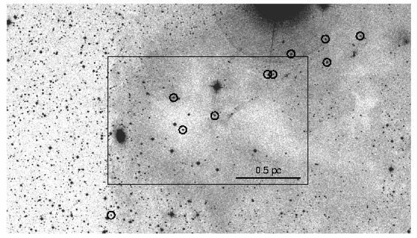
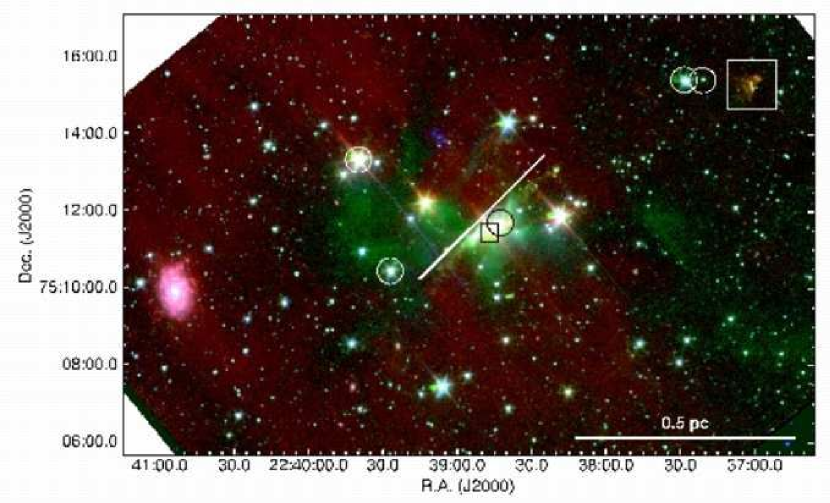
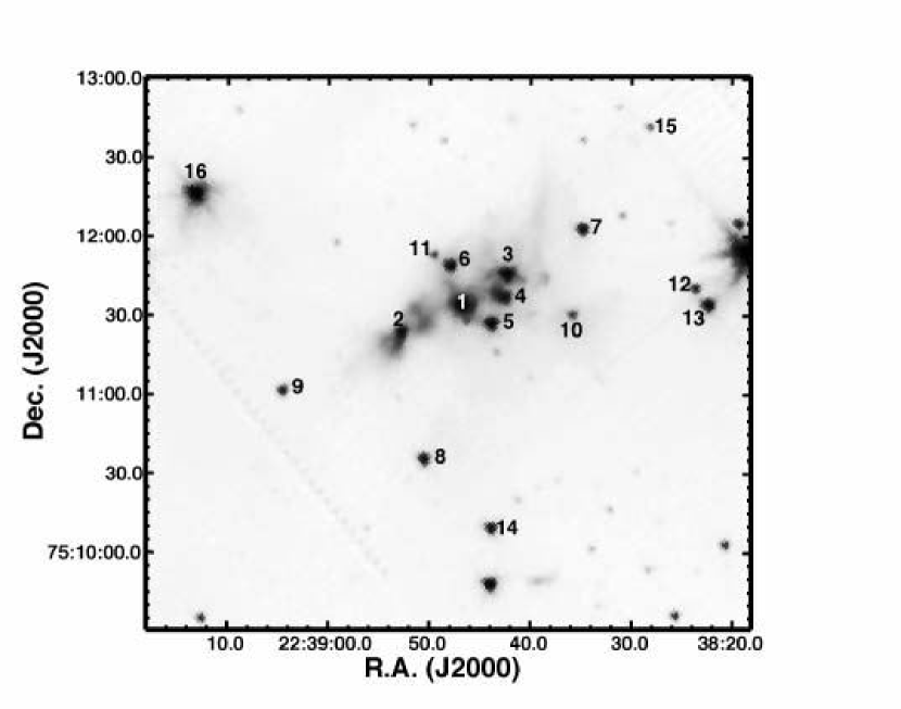
Figure 1 shows the Digitized Sky Survey (DSS) R-band image around L1251E, with stars identified as “H$\alpha$ stars” by Kun & Prusti (1993) indicated. In comparison, Figure 2 shows the IRAC three-color image of 3.6, 4.5, and 8.0 µm, revealing a small group of infrared sources associated with L1251B, at the location of one H$\alpha$ star and adjacent to the position of IRAS 22376+7455. The spiral galaxy, UGC 12160 (Cotton et al. 1999), is located in the east edge of Figure 2. To the northwest, Figure 2 also shows the Herbig-Haro (HH) object HH373, which shows up in the longer wavelength bands as well as at 4.5 $\mu$m. The extended green color seen in Figure 2 all around the central group is dominated by scattered light with some contribution from shocked gas associated with jets and outflows. A jet-like feature, $\sim$0.3 pc long and aligned in the SE-NW direction, is seen centered near the IRAS position, with an emission knot at its northwestern tip. There is also green, arc-shaped emission $\sim$2′ ($\sim$0.17 pc) south of L1251B in Figure 2, which is associated with HH189C (Eiroa et al. 1994) and might be caused by a jet from one protostar of the group. There are red-free green patches, indicating absorption against the background 8.0 µm PAH emission, to the east of the central group. These patches are dominated by scattered light and seen as optically dark locations in the DSS R-band image (Figure 1) and as submillimeter bright locations in the 850 µm emission map (see Figure 3).

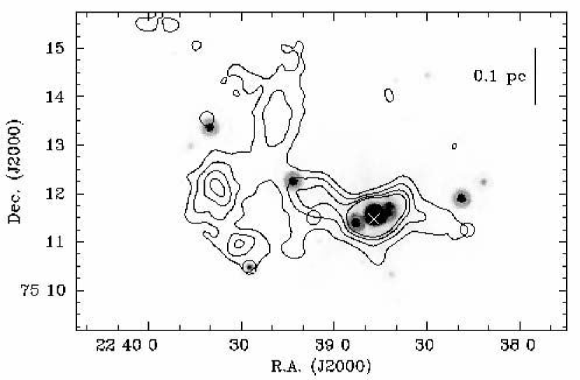
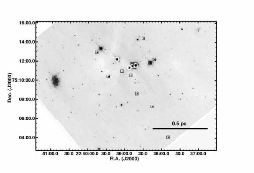
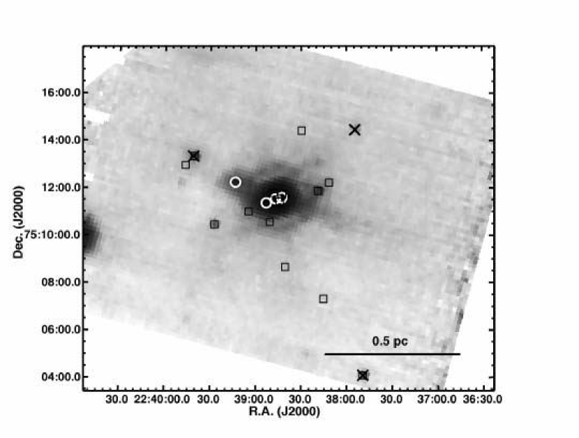
In Figure 3, extended emission at 850 µm in the L1251E region is shown with contours on top of the MIPS 24 $\micron$ image. The 850 $\micron$ emission peaks very strongly at L1251B, which we call the “west core.” There are 3-4 other, weaker, 850 $\mu$m peaks within 200″ of L1251B to the east (NE to ESE). The brightest of these, which we call the “east core”, is located $\sim$180″ east of L1251B. Three 24 µm sources are located east of L1251B region and two are coincident with T Tauri-like objects with H$\alpha$ emission (Kun & Prusti 1993). There are no sources, however, in the IRAC and MIPS bands around the weaker 850 $\mu$m emission peaks. T$\acute{\rm o}$th & Walmsley (1996) showed that the east core has a higher column density of NH₃ than the west core (L1251B) and that both may be gravitationally unstable. Therefore, the east core may be prestellar in nature, i.e., a potential site of future star formation. Only three (two T Tauri-like objects and IRAS 22376+7455) of five IRAS point sources have corresponding objects at 24 $\micron$ in Figure 3. The other two IRAS point sources have not been detected either in IRAC or MIPS bands.

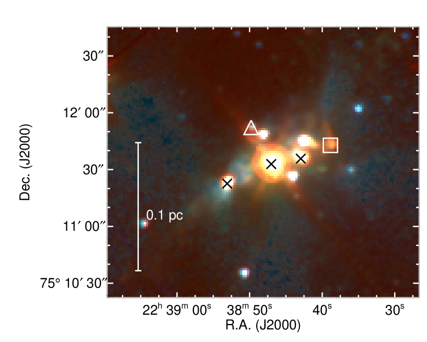
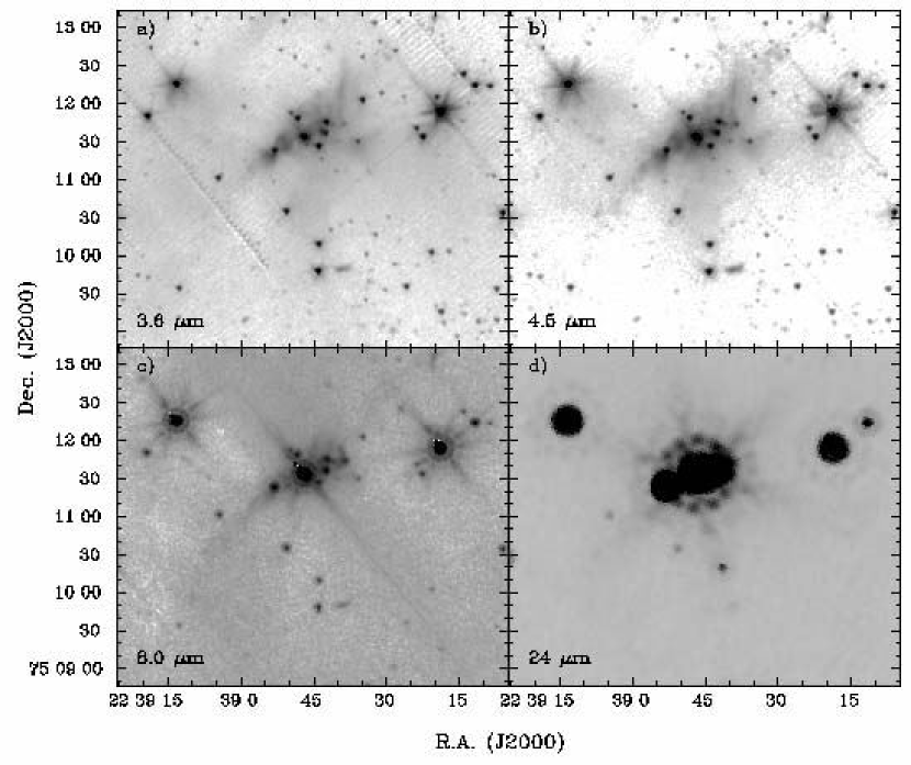
Figure 4 shows the zoomed-in three-color composite image of L1251B, the central group of Figure 2, while Figure 5 shows separately the IRAC 3.6 µm, 4.5 µm, and the 5.8 µm band images and the MIPS 24 µm band image around L1251B. There are 8 point-like sources in the central region of Figure 4. The source denoted with a triangle at (22^h38^m49.7^s, +75^∘11′52.7″) is detected as a point source only in the IRAC 3.6 and 4.5 µm bands, however. The red source denoted with a square at (22^h38^m38.7^s, +75^∘11′43.9″) is weak and nebulous in the short IRAC bands, but in the IRAC 8.0 µm band, the source becomes stronger and point-like on top of arc-shaped emission. This source might be an infrared source analog to a HH object. Therefore, there are 6 bright sources detected in all IRAC bands as point sources, and among them, only the three sources, each marked with an X, are clearly identified at 24 µm. IRAS 22376+7455 covers the whole group because of the poor resolution of the IRAS observations. The coordinates of the IRAS source, however, are closest to the brightest IRAC source, which we name “L1251B-IRS1.” A bipolar structure associated with the SE source, which we name “L1251B-IRS2,” is clearly seen, and it is probably due to scattered light from a bipolar outflow cavity. The opening of the bipolar nebula is similar in direction to that of the jet seen (with the white line) in Figure 2, suggesting that IRAS 22376+7455 may not be the only driver of the large CO outflow, as previously believed. (Note that the bipolar nebula is not associated with IRS1.) We will discuss this situation further in Paper II.

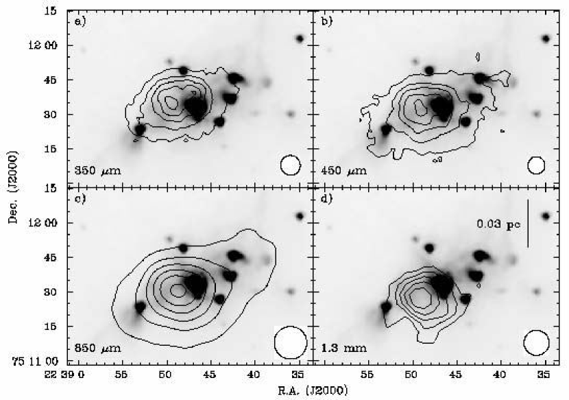
Figure 6 shows the continuum emission around L1251B at various (sub)millimeter wavelengths on top of the IRAC 4.5 µm band image. The IRAC image shows the bipolar nebula of IRS2 and diffuse emission over the region likely due to scattering. There are two intensity peaks at 350 $\micron$ and 450 $\micron$; the stronger peak does not have a corresponding IRAC source and the weaker peak seems related to IRS1, the brightest IRAC source. The emission at 850 $\micron$ and 1300 $\micron$, however, has only one peak corresponding to the stronger peak at 350 $\micron$ and 450 $\micron$. The stronger intensity peak is located between IRS1 and IRS2. (As we show in Paper II, this position is coincident with a peak of N₂H⁺ emission, which traces cold, dense regions.) The stronger peak may be a high column density peak of the envelope. The weaker peak, however, may be heated primarily by IRS1 since it disappears at longer wavelengths.

If the intensity distributions of dust continuum at various wavelengths are compared, a shift is seen in the positions of intensity peaks with wavelength from north to south. The pointing error of the 350 $\micron$ emission is relatively large, so it could be adjusted in position to match its weaker peak to the 450 $\micron$ second peak. A systematic shift of intensity peaks with wavelength, however, cannot be explained only by pointing errors. The angular separation ($\sim 6\mbox{\arcsec}$) between the 1.3 mm intensity peak and the stronger 450 $\micron$ peak is much greater than the pointing error ($<3\mbox{\arcsec}$) of the 450 $\micron$ and 1.3 mm observations. Such a shift may involve a systematic variation of physical conditions such as density, temperature, or opacity.

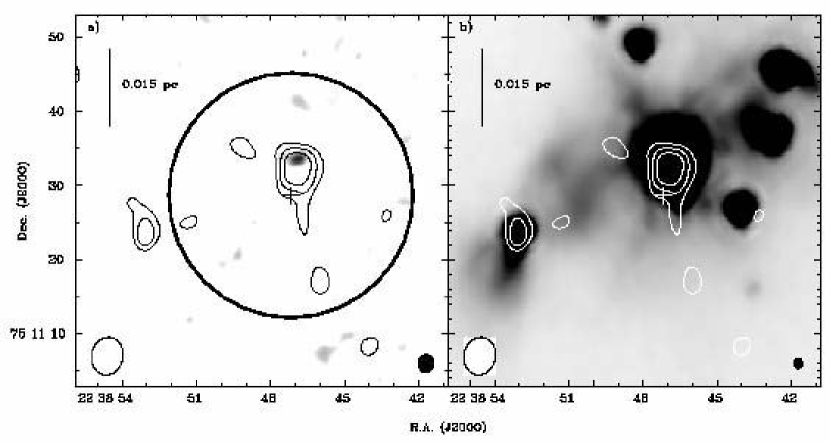
Figure 7a shows the dust continuum intensities observed with the OVRO array at 3 mm and 1.3 mm. Such data can trace dust from deeply embedded disks or the interiors of envelopes. The two intensity peaks at 3 mm correspond to IRS1 and IRS2, as seen in Figure 7b. At 1.3 mm, however, IRS2 is located beyond of the FWHM of the primary beam at the coordinates of IRAS 22376+7455. The OVRO results also show that IRS1 is located 5″ north of the coordinates given in the IRAS point source catalog.

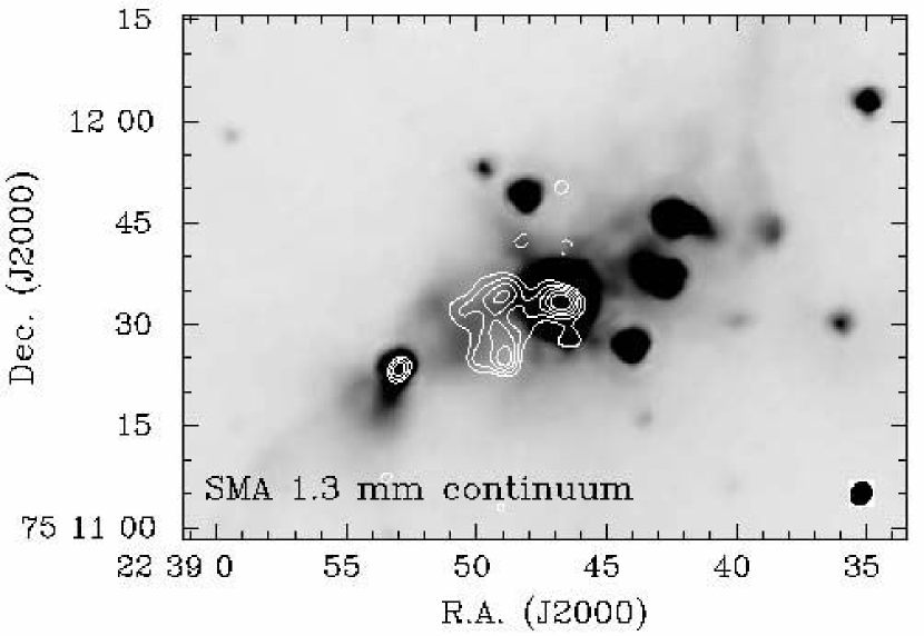
The result of the SMA observation in the 1.3 mm continuum is shown in Figure 8. Four detections are seen. The brighter two detections are compact and coincident with IRS1 and IRS2 as seen in the OVRO 3 mm data, so deeply embedded disk components of IRS1 and IRS2 are traced with these interferometric observations. The fainter two detections are more extended and peak to the east and southeast of IRS1, and they were detected separately in the USB and LSB data sets which were reduced independently. The faint extended emission associated with these two latter sources is coincident with the brightest regions of integrated N₂H⁺ 1$-$0 intensity seen in our OVRO map (see Paper II). No 1.3 mm continuum emission is seen associated with any other near-infrared sources. The two weaker intensity peaks at 1.3 mm are also consistent with the stronger peaks of the 350 and 450 µm emission and the peaks of 830 and 1300 µm emission observed with single dishes. Therefore, the two intensity peaks newly detected in the SMA 1.3 mm observation are probably the highest densities of the L1251B envelope, whose extended emission was resolved out by the interferometers. If true, these sources may be prestellar condensations and not detected at 3 mm with OVRO due to low sensitivity.

Interestingly, however, the two weaker SMA 1.3 mm emission peaks were not detected in the OVRO 1.3 mm observation. The two SMA 1.3 mm peaks lie within the FWHM of the OVRO primary beam, and the 1 $\sigma$ sensitivities of both OVRO and SMA 1.3 mm observations are the same although the peak intensity of IRS1 in the OVRO 1.3 mm observation (14 mJy beam^-1) is less than a half of that in the SMA 1.3 mm observation (34 mJy beam^-1). We tested the SMA data by excluding spatial frequencies lower than the lowest spatial frequency of the OVRO data, and found that extended 1.3 mm emission between IRS1 and IRS2 disappeared in the resulting images. This discrepancy is therefore caused mainly by shorter baselines in the SMA data ensemble, which is more sensitive to extended structure. Remaining discrepancies are likely the result of the flux calibration not being as accurate as for the SMA data since flux calibrators were monitored at 1 mm less frequently at OVRO. As a result, the flux of IRS1 from the SMA observation is stronger than that from the OVRO observation. Other complementary data, such as continuum data at 345 GHz (observed with the SMA), are necessary to understand the physical conditions of two extended prestellar condensations.

4 ANALYSIS

For general analysis with color-color and color-magnitude diagrams, we include all sources in Figure 2, but focus on sources around L1251B for more detailed analysis of their spectral energy distributions (SEDs). Figure 9 shows our selected identification numbers for sources around L1251B. Here, 6 sources (from 1 to 6) within the L1251B dense core, which is detected in submillimeter continuum with single-dish telescopes (Figure 6) and focused on in Paper II, are named as L1251B-IRS1, -IRS2, -IRS3, and so on. Again, IRS1 is the brightest IRAC source, and IRS2 is the object associated with the NIR bipolar nebula. Other sources (from 7 to 16) outside L1251B are just named as source 7, source 8, and so on.

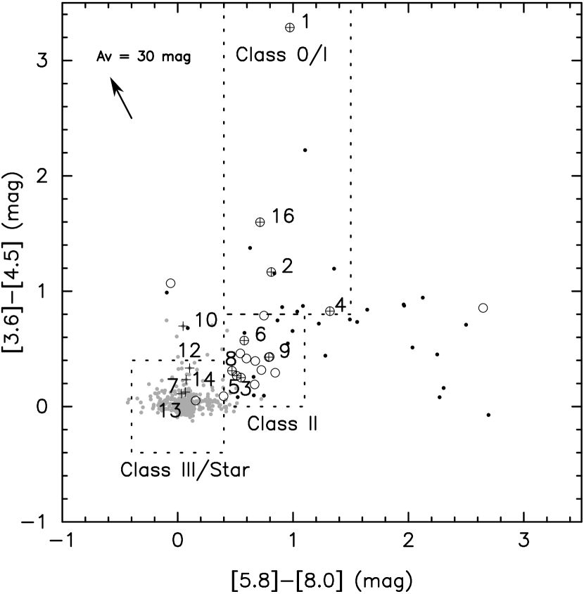
Allen et al. (2004) described how the [3.6]$-$[4.5] vs. [5.8]$-$[8.0] color-color diagram can be used to identify the evolutionary stages of sources detected by IRAC. Figure 10 shows such a color-color diagram for sources in L1251E, along with domains of color representative of objects from various pre-main-sequence classes, similar to those identified by Allen et al. For example, we identify Class II sources in L1251B with the color range 0 $<$ [3.6]$-$[4.5] $<$ 0.8 and 0.4 $<$ [5.8]$-$[8.0] $<$ 1.1, and Class 0/I sources within color range of [3.6]$-$[4.5] $>$ 0.8 and 0.4 $<$ [5.8]$-$[8.0] $<$ 1.5. This latter range covers a smaller area than that of the Class 0/I models shown in Figure 4 of Allen et al., since none of the sources with [5.8]$-$[8.0] $>$ 1.5 are in the L1251B core where Class 0/I sources are most likely located. According to these color ranges, there are 33 Class II sources and 10 Class 0/I sources for L1251E as a whole.

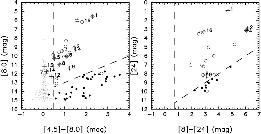
Background galaxies can be detected with the sensitivity of the c2d observations, and may have colors within the expected ranges of Class 0/I or Class II sources (Eisenhardt et al. 2004). To remove potential galaxy “contamination,” we require the YSO candidates fulfill either one of two sets of color-magnitude criteria: (1) [4.5]$-$[8.0] $>$ 0.5 and [8.0] $<$ (14 $-$ [4.5]$-$[8.0]) or (2) [8.0]$-$[24] $>$ 0.7 and [24] $<$ (12 $-$ [24]$-$[8.0]). These criteria are derived from a comparison (Harvey et al. 2006; Jorgensen et al. 2006) between the c2d data and the data from the SST SWIRE Legacy Project. The SWIRE project is a deep imaging survey at the Galactic Pole and provides an essentially YSO-free sample, while the regions observed by the c2d project contain a fair amount of YSOs. The comparison between the two data sets show that the SWIRE sources are extremely depleted in the color-magnitude space defined by the two sets of color-magnitude criteria. Two sets of color-criteria are shown in Figure 11 with dashed lines. The level of the criteria are chosen so that (1) 95% of the SWIRE sources with [4.5]$-$[8.0] $>$ 0.5 are under the diagonal line in the left panel and (2) 95% of the SWIRE sources with [8]$-$[24] $>$ 0.7 are under the diagonal line in the right panel. Under these criteria only 15 SWIRE sources per square degree could be potentially mis-identified as YSO candidates. (A detailed description of these selection criteria is provided in Lai et al., in preparation). The probability of the faint YSOs missed by these criteria cannot be assessed at this point due to lack of knowledge of faint YSO populations.

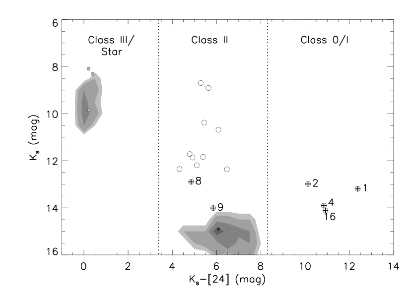
Figure 11 shows the distribution of the sources detected in L1251E with peak signal-to-noise ratios $\geq$ 7 in all IRAC bands in [8.0] vs. [4.5]$-$[8.0] and [24] vs. [8.0]$-$[24] color-magnitude diagrams with boundaries indicating the two SWIRE-based sets of color-magnitude criteria. Sources located in the upper right corner in either color-magnitude diagram are selected as YSO candidates, while those to the left are likely stars and those remaining are likely galaxies. (Note that the YSO candidate under the dashed lines in the extragalactic region in one color-magnitude diagram must be located above the dashed line in the other color-magnitude diagram.) 21 objects are identified as YSOs based on these two color-magnitude diagrams. As in Figure 10, sources identified with plus symbols in Figure 11 are those around the L1251B core. After removing the likely extragalactic sources in Figure 10, the number of Class 0/I candidates is reduced to 4 and all of them are located around the L1251B core. Also, the number of Class II candidates reduces to 14 in the L1251E region and to 5 around the L1251B core. Three of the YSOs identified by the color-magnitude diagrams (Figure 11) do not fall into the criteria of Class 0/I or Class II in the color-color diagram (Figure 10) and located far from L1251B. Figure 12 shows the spatial distribution of YSO candidates in L1251E, and the fluxes of these YSO candidates are listed in Table 2 and 3. The flux uncertainty is $\sim$15%.

In summary, we are adopting the color criteria as given in the c2d catalog and their source classification. First, the c2d color-magnitude diagrams (Figure 11), which do not provide the information on Classes, are used to extract YSO candidates, and as a next step to classify the evolutionary stages of the YSO candidates, the color-color diagram seen in Figure 10 is used. Finally, 4 Class 0/I and 14 Class II candidates are classified in L1251E even though 21 YSO candidates are extracted from the c2d color-magnitude diagrams. The galaxy contamination rate of our YSO candidate selection criteria obtained from the SWIRE data is 15 sources per square degree, thus the 0.4^∘$\times$0.35^∘ Spitzer image of L1251E should have 2.1 mis-identified YSO candidates. Therefore, excluding 3 YSO candidates (including one known HH object) is consistent with the prediction of our adopted criteria.

Among the sources around the L1251B core, Figures 10 and 11 indicate that IRS1, IRS2, and source 16 are in Class 0/I, IRS3, IRS5, IRS6, and sources 8 and 9 are in Class II, and sources 7, 10, 12, 13, and 14 are stars. We note that Source 11 is detected only in the IRAC 3.6 $\mu$m and 4.5 $\mu$m bands. In Figure 10, some sources with [5.8]$-$[8.0] $>$ 1.5 have [3.6]$-$[4.5] $<$ 1; from the c2d criteria, all of these, except for one source (see below), are likely background galaxies. We note that IRS1 has a much redder [3.6]$-$[4.5] color than a [5.8]$-$[8.0] color, perhaps caused by absorption within its massive envelope by the 10 $\mu$m silicate feature that overlaps with the IRAC 8.0 $\mu$m band (Allen et al. 2004). Similar colors are seen in other deeply embedded sources (Jorgensen et al. 2006; Dunham et al. 2006).

Color-color identification of evolutionary state is based on presumptions about the physical characteristics of each object, and this could lead to some misclassifications. For example, the exceptional source (noted above) in Figure 10 with [5.8]$-$[8.0] $>$ 1.5 and [3.6]$-$[4.5] $<$ 1 may be a Class 0/I YSO with an very low envelope density (see Fig. 1 of Allen et al. 2004). In addition, the YSO candidate with [3.6]$-$[4.5]$=$11 and [5.8]$-$[8.0]$=$$-$0.1 also might be a Class 0/I object with a very low central luminosity, a low envelope density, and a large centrifugal radius. Finally, the YSO candidate with colors similar to those of Class III objects or stars (i.e., Class III/Star) may be a Class II source with a low disk accretion rate and a low inclination. We expect the number of misclassifications to be minimal, though calibration of color-color diagrams through modeling the SEDs of specific sources therein would be welcome.

Figure 13 is a $K$ vs. $K-[24]$ color-magnitude diagram which is used to check the possibility of confusion between our sources and background galaxies. All YSO candidates detected clearly at 24 µm are bright or red enough to be separated clearly from background galaxies. IRS1, IRS2, IRS4, and source 16, which are in Class 0/I and were detected separately by MIPS are very red. IRS1, IRS2, and IRS4 are clearly the youngest most embedded members of L1251B, and they are possibly still forming out of the rapidly rotating envelope and through interaction with outflows (see Paper II). IRS3, IRS5, and IRS6, however, were not clearly detected at 24 µm even though they are classified as Class II and are close in projection to IRS1, IRS2, and IRS4. These may comprise an older population located at the outer boundary of the dense L1251B region.

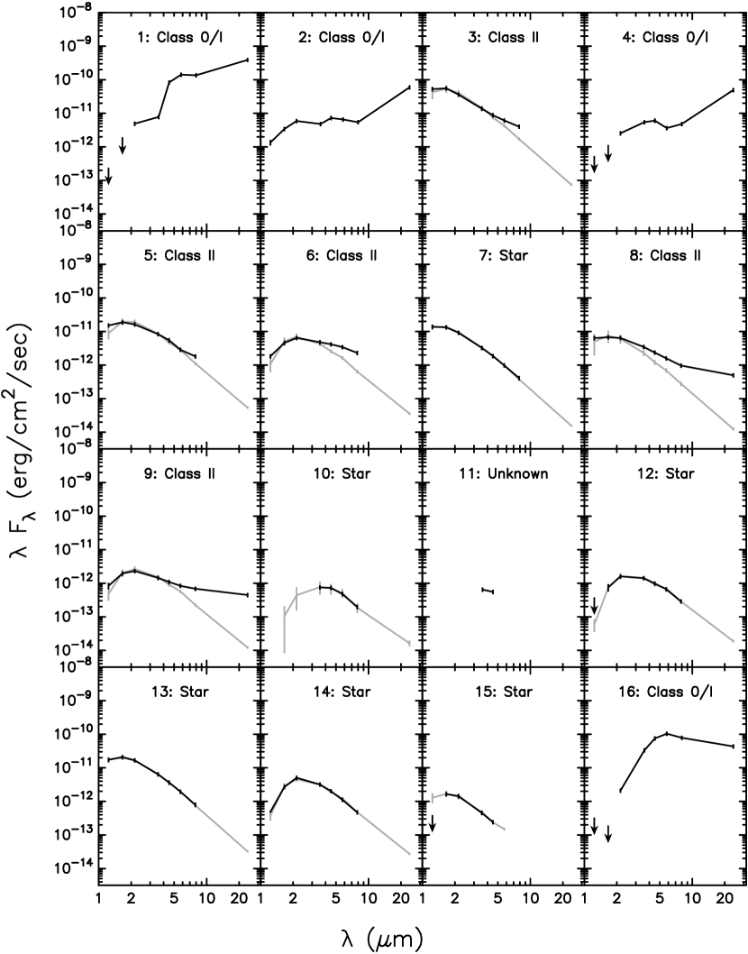
Figure 14 shows stellar model fits on top of SEDs of sources around L1251B. According to the c2d stellar model fits, sources 7, 10, 12, 13, 14, and 15 are possible foreground or background stars reddened by some extinction. Based on the description of the source type by catalogs (Evans et al. 2006; Lai et al. in preparation), IRS1, IRS2, IRS4, and source 16 are potential Class 0/I objects and IRS3, IRS5, IRS6, and sources 8 and 9 are possibly Class II, star/disk objects. These results are consistent with results from the color-color diagram shown in Figure 10.

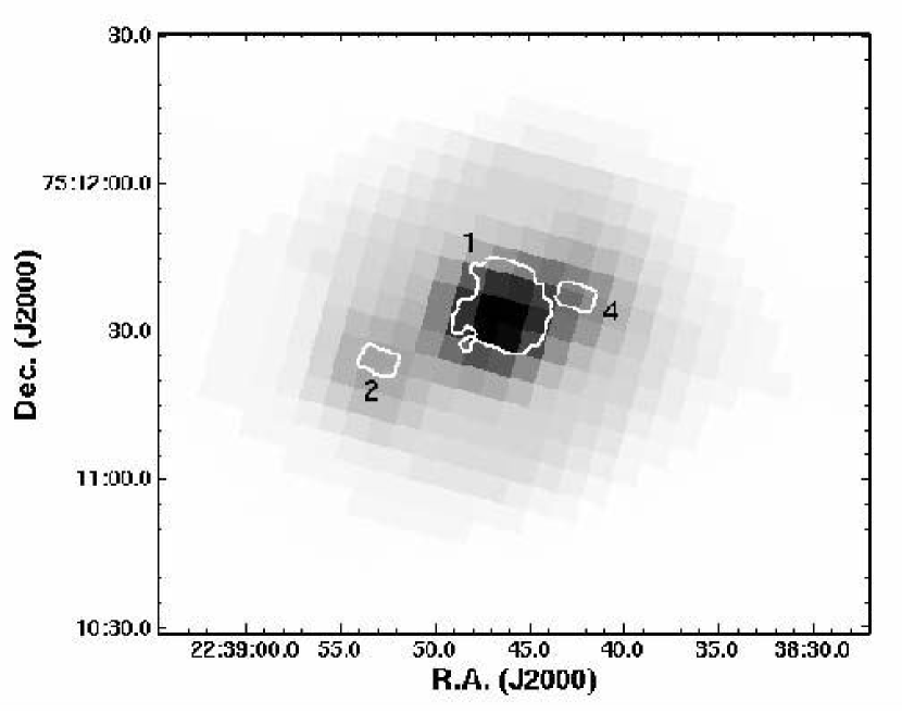
The MIPS 70 µm image for L1251E is shown in Figure 15a. Some of the YSO candidates show diffuse or point source-like emission at 70 µm, though the emission from the inner L1251B region is confused by IRS1, IRS2, and IRS4. To estimate the 70 $\mu$m fluxes of these unresolved sources, 70 $\mu$m fluxes were measured within a 24 $\mu$m intensity contour chosen to separate the three sources (see Figure 15b). Given the ratios of flux between sources enclosed by this contour, the total 70 $\mu$m flux, as measured by annular photometry, was divided among the three sources. (In applying this procedure, we have assumed that the spatial extent of the 70 $\mu$m sources matches that of the 24 $\mu$m resolved sources.) Note that the extent of emission from IRS1 will influence the flux measurements of IRS2 and IRS4. To mitigate the influence of the extended emission from IRS1, therefore, the IRS1 flux has been fitted with a Gaussian profile, and the relative fluxes from IRS2 and IRS4 above the wings of the IRS1 profile have been measured.

We also applied the 70 $\micron$ flux ratios to estimate the 350, 450, and 850 $\micron$ fluxes of the three sources. In Table 4, we list flux densities from 1.2 to 850 µm of IRS1, IRS2 and IRS4 and in Table 5, we list bolometric luminosities ($L_{bol}$), bolometric temperatures ($T_{bol}$), and $L_{smm}/L_{bol}$, where $L_{smm}$ is the luminosity at $\lambda>350$ µm, for these sources based on their SEDs. According to the results, IRS1 is the dominant luminosity source in L1251B by a factor of $\sim$10. Young et al. (2003) found that L1251B should be in Class 0 based on $T_{bol}$ (64 K) and $L_{smm}/L_{bol}$ (0.01), which were calculated from single dish submillimeter continuum observations, and assuming only one heating source (IRAS 22376+7455). However, as seen in Table 5, IRS1, IRS2, and IRS4 are classified to Class I objects based on $T_{bol}$ ($>70$ K) while they are still categorized to Class 0 based on $L_{smm}/L_{bol}$ ($>0.005$). The bolometric luminosities of IRS1 and IRS2 include submillimeter emission from their respective envelopes, but these may also include such emission from the prestellar objects between IRS1 and IRS2. (Such prestellar objects do not have emission at shorter wavelengths to contribute to bolometric luminosities.) Given the proximity of these objects to IRS1, their possible contributions likely affect the bolometric luminosity estimate of IRS1 more than any other in L1251B source. Hence, the luminosity of IRS1 of 10 L_⊙ is likely an upper limit. In contrast, if fluxes at submillimeter wavelengths ($\lambda\geqq 350$ µm) are not considered, the lower limit of the luminosity of IRS1 is 5 L_⊙. To quantify the amount of contribution of fluxes at submillimeter wavelengths from each source, detail models are necessary.

5 DISCUSSION

In L1251E, about 30 point sources were detected in the MIPS 24 µm band, and $\sim$75% of these were classified as YSO candidates (see Figure 11). Based on color-color classifications (see Figure 10), about 22% and 78% of the YSOs in L1251E are in Class 0/I and Class II respectively. (A few YSO candidates, however, have colors that do not fall into the Class 0/I or Class II classifications.) Within L1251B, however, 6 YSOs were detected half of them are classified as Class 0/I candidates, and the other half are classified as Class II protostars. The whole field size of the MIPS observation is about 2.5 pc², so the number density of YSOs in L1251E is about 10 pc^-2. The spatial number density of YSOs in L1251B exceeds that in the whole L1251E region by two orders of magnitude. The area used for the number density calculation in L1251B is $\sim$0.01 pc², which covers emission at submillimeter wavelengths shown in Figure 6.

We compare L1251E and L1251B with two larger cluster forming regions observed with the SST: NGC 2264 (Teixeira et al. 2006) and Perseus (Jorgensen et al. 2006). For this, we concentrate on the “Spokes” cluster in NGC 2264 and NGC 1333 and IC 348 in Perseus. The Spokes cluster ($\sim$2 pc²) and NGC 1333 ($\sim$3.2 pc²) have similar spatial areas to L1251E ($\sim$2.5 pc²), and IC 348 has about three times bigger area ($\sim$6.9 pc²) than L1251E.

Forty YSOs were detected in the Spokes cluster, which is the densest part of NGC 2264, in the MIPS 24 µm band. The area of the Spokes cluster is $\sim$2 pc², yielding a YSO number density of $\sim$20 pc^-2, greater than that of L1251E by a factor of 2. In NGC 2264, however, the magnitude of the weakest YSO detected at 24 µm is about 6.7 mag. With a similar restriction (and keeping in mind the factor of $\sim$2 in distance between regions), the number of point sources detected in the MIPS 24 micron band with [24] $<$ 6.7 in L1251E is 10, and all are classified as YSO candidates (see Figure 11). Based on this number, the spatial number density of YSO candidates in L1251E is $\sim$4 pc^-2, i.e., smaller than that in the Spokes cluster by a factor of 5. Despite this difference in spatial number densities, the fraction of Class 0/I candidates in L1251E ($\sim$22%) is not very different. In addition, the fraction of Class 0/I candidates in L1251B (50%), the densest region in L1251E, is not different from that of the dense region around IRAS 12 in NGC 2264 ($\sim$60%).

IC 348 and NGC 1333 show similar number densities of YSOs to that in L1251E. The fractions of Class 0/I candidates in IC 348 and NGC 1333 are about 14% and 36%, respectively. In the remaining cloud outside IC 348 and NGC 1333, however, the fraction is about 47%, indicative of different formation timescales over Perseus. In summary, therefore, the number density of YSOs in L1251E is similar to those in active star forming regions of NGC 2264 and Perseus.

L1251B has three Class 0/I members (IRS1, IRS2, and IRS4), which have been detected at 24 µm, and three more Class II members (IRS3, IRS5, and IRS6) are located in projection inside L1251B in the IRAC images (e.g., see Figures 3 or 4). The average projected distance among 18 YSOs in L1251E is about 213″ with the standard deviation of $\sim$148″  whereas the average projected distance of 6 YSOs in L1251B is about 24″  indicating clustering. Single dish submillimeter continuum emission, which traces dense envelope material, covers the 6 YSOs of L1251B with intensity peaks between IRS1 and IRS2. In addition, two sources located between IRS1 and IRS2 have been newly detected at 1.3 mm with the SMA. They are not associated to any IRAC or MIPS source; and are possibly prestellar condensations. The shift of intensity peaks in the submillimeter continuum emission (see Figure 6 and §3) observed with single dish telescopes seems related to the variation of physical properties of the two prestellar condensations. For example, the shift of intensity peaks from the north to the south with wavelength can be explained if the prestellar source at the north has a higher temperature than the other one. These observed features covering various evolutionary stages (from prestellar to Class II) suggest that fragmentations during gravitational collapse of a dense molecular core (Boss 1997; Machida et al. 2005) can explain the formation of this small group of pre- and protostellar objects in L1251B. Class 0/I objects in L1251B might help the formation of further prestellar condensations since the external pressure resulting from a previous star formation event could reduce Jeans fragmentation length scales in the remaining matter for the next incidence of star formation (Ward-Thompson et al. 2006 and references). We examine the molecular line data in Paper II to understand how dynamics and chemistry are distributed in L1251B, and how the group members of L1251B are interacting.

Many YSO candidates in various evolutionary stages are distributed all over the extended L1251E region. In addition, the east core has a radius of about 0.3 pc and may harbor future star formation (see Paper II). This suggests that L1251E is a possible example of low-mass cluster formation, and L1251B, which is a small group of pre- and protostellar objects, is just part of the larger, on-going cluster formation.

6 SUMMARY

L1251E, the densest C¹⁸O core of L1251, has been observed by the SST as part of the SST c2d Legacy project. The most interesting region in L1251E is L1251B, which has been revealed by the SST to be a small group of protostars. We have compared the SST data with other continuum data to study L1251B more comprehensively. The summary of our results is as follows:

1. L1251E contains at least two cores, a western one coincident with L1251B and an eastern one detected at 850 µm continuum. No source has been detected in the IRAC or MIPS bands toward the east core, suggesting it is starless. Asymmetrically blue line profiles (see Paper II) have been detected toward the eastern core, however, that are suggestive of infall motions.

2. About 20 YSO candidates (4 in Class 0/I, 14 in Class II, and 3 unclassified YSOs) are distributed all over L1251E, suggesting L1251E is a possible example of low mass clustered star formation.

3. L1251E has a surface number density of young stellar objects of $\sim$10 pc^-2, not very different from those seen in the Spokes cluster of NGC 2264 and the most active star forming regions of Perseus, IC 348 and NGC 1333. The spatial number density in L1251B is, however, larger than that of L1251E by about two orders of magnitude, indicative of highly concentrated star formation. The fractions of Class 0/I candidates in aL1251E and L1251B are similar to those in and around the Spokes cluster, but the fraction in Perseus varies from region to region.

4. Six sources located in projection within L1251B were detected in all IRAC bands but only IRS1, IRS2 and IRS4 are detected clearly at 24 µm (with MIPS) and classified as Class 0/I candidates. IRS2 is associated with a near-infrared bipolar nebula.

5. Dust continuum emission maps made at 350 µm and 450 µm show two intensity peaks in L1251B. The stronger peak is not associated with any IRAC source but the weaker peak is associated with IRS1, the brightest object in L1251B. The stronger peak is located between IRS1 and IRS2. The weaker peak disappears at 850 µm and 1300 µm and the distribution of continuum emission around the stronger peak becomes more spherical (and shifts to the south with increasing wavelength.) Therefore, the stronger peak seems to be a column density peak, and the weaker peak is possibly from dust heated by IRS1.

6. IRS1 and IRS2 are detected as compact objects in the OVRO 3 mm and the SMA 1.3 mm observations, indicating that they are deeply embedded disk sources. In addition, two sources have been newly detected between IRS1 and IRS2 at 1.3 mm with the SMA. These two sources confirm that the stronger intensity peaks at 350 and 450 µm and intensity peaks at 850 and 1300 µm are column density peaks. The positional shift of continuum density peaks with wavelength is possibly caused by a temperature difference between the two newly detected sources.

Table 1: OVRO and SMA Observational Summary

		Gaussian	Synthesized	Synthesized
	Bandwidth	Taper FWHM	Beam FWHM	Beam P.A.	1 $\sigma$ rms
Tracer	(GHz)	(″ $\times$ ″)	(″ $\times$ ″)	(∘)	(Jy beam-1)
OVRO 1.33 mm	2	1.60 $\times$ 1.60	2.4 $\times$ 2.3	309	0.003
OVRO 2.95 mm	2	3.25 $\times$ 3.25	5.2 $\times$ 4.8	321	0.0007
SMA 1.33 mm	4	$\cdots$	4.1 $\times$ 3.5	339	0.003

Table 2: Class 0/I candidates in L1251E

RA (J2000)	Dec (J2000)			Fluxes (mJy)			ID
(h m s)	(∘ $\arcmin$ $\arcsec$)	IRAC 1	IRAC 2	IRAC 3	IRAC 4	MIPS 1
22 38 42.8	75 11 36.8	6.54e+00	9.06e+00	7.02e+00	1.28e+01	3.95e+02	L1251B-IRS4
22 38 46.9	75 11 33.9	9.37e+00	1.25e+02	2.74e+02	3.63e+02	3.12e+03	L1251B-IRS1
22 38 53.0	75 11 23.5	5.76e+00	1.09e+01	1.27e+01	1.45e+01	4.74e+02	L1251B-IRS2
22 39 13.3	75 12 15.8	4.01e+01	1.13e+02	2.01e+02	2.10e+02	3.48e+02	16

Table 3: Class II candidates in L1251E

RA (J2000)	Dec (J2000)			Fluxes (mJy)			ID
(h m s)	(∘ $\arcmin$ $\arcsec$)	IRAC 1	IRAC 2	IRAC 3	IRAC 4	MIPS 1
22 37 49.6	75  4  6.4	1.85e+01	1.30e+01	9.02e+00	7.04e+00	9.55e+01
22 38 11.6	75 12 14.6	8.45e+00	8.13e+00	7.83e+00	8.83e+00	2.88e+01
22 38 15.2	75  7 20.4	1.39e+01	1.32e+01	9.82e+00	9.20e+00	1.73e+01
22 38 18.7	75 11 53.8	1.22e+02	1.63e+02	2.32e+02	2.50e+02	3.22e+02
22 38 29.6	75 14 26.7	8.45e+00	7.16e+00	6.32e+00	7.45e+00	1.09e+01
22 38 40.5	75  8 41.3	7.34e+00	6.83e+00	5.84e+00	5.87e+00	9.64e+00
22 38 42.5	75 11 45.5	1.62e+01	1.32e+01	1.17e+01	1.05e+01	5.66e+01	L1251B-IRS3
22 38 44.0	75 11 26.8	9.91e+00	8.20e+00	5.46e+00	4.73e+00	3.91e+01	L1251B-IRS5
22 38 48.1	75 11 48.8	5.68e+00	6.22e+00	6.54e+00	6.02e+00	-1.92E+00	L1251B-IRS6
22 38 50.7	75 10 35.3	4.10e+00	3.53e+00	3.03e+00	2.53e+00	3.97e+00	8
22 39 4.7	75 11  1.2	1.71e+00	1.64e+00	1.60e+00	1.79e+00	3.57e+00	9
22 39 27.2	75 10 28.4	3.74e+01	3.24e+01	2.88e+01	3.04e+01	6.99e+01
22 39 40.3	75 13 21.6	1.82e+01	1.80e+01	1.86e+01	1.66e+01	1.11e+01
22 39 46.4	75 12 58.7	2.15e+02	1.66e+02	2.43e+02	2.43e+02	2.84e+02

Table 4: Flux densities (mJy) of L1251B sources

Wavelength (µm)	L1251B-IRS1	L1251B-IRS2	L1251B-IRS4
1.235	9.47e-02	5.55e-01	2.13e-01
1.662	1.03e+00	1.89e+00	6.04e-01
2.159	3.52e+00	4.25e+00	1.83e+00
3.555	9.37e+00	5.76e+00	6.54e+00
4.493	1.25e+02	1.09e+01	9.06e+00
5.731	2.74e+02	1.27e+01	7.02e+00
7.872	3.63e+02	1.45e+01	1.28e+01
24.00	3.12e+03	4.74e+02	3.95e+02
70.00	2.5e+04	8.5e+02	1.4e+03
350.0	4.2e+04	2.8e+03	4.0e+03
450.0	2.1e+04	1.3e+03	2.1e+03
850.0	5.8e+03	3.4e+02	5.8e+02

Table 5: Luminosities and bolometric temperatures of L1251B sources

	L1251B-IRS1	L1251B-IRS2	L1251B-IRS4
$\rm L_{bol}$ (L⊙)	10	0.6	0.8
$\rm T_{bol}$ (K)	87	140	98
$\rm L_{smm}\tablenotemark{a}/L_{bol}$	0.03	0.03	0.04

Figure 1: The Digitized Sky Survey (DSS) $R-$band image of L1251E. The box indicates the field of view of Figure 2 and the circles indicate H$\alpha$ stars from Kun & Prusti (1993).

Figure 2: Three-color composite SST image of L1251E. The IRAC 3.6, 4.5, and 8.0 $\micron$ data are presented respectively as blue, green, and red. The small box represents the position of IRAS 22376+7455 and the large box includes the Herbig-Haro (HH) object, HH 373. The circles denote the same H$\alpha$ stars shown in Figure 1. The H$\alpha$ star with the black box seems consistent with IRS3 (Figure 9). The red spiral galaxy located at (22^h40^m54.6^s, +75^∘09′52.5″) is UGC 12160 (Cotton et al. 1999). The white line, which is in the direction of SE-NW and centered around IRSA 22376+7455, indicates a jet-like feature, $\sim$0.3 pc long.

Figure 3: Mid-infrared and submillimeter continuum emission in L1251B. Emission at $\lambda$ = 24 $\mu$m obtained with MIPS is shown in greyscale while emission at $\lambda$ = 850 $\mu$m obtained with SCUBA is shown in black contours. The greyscale range is 15-50 MJy sr^-1 and the contours begin at 0.05 Jy beam^-1 and increase in steps of 0.05 Jy beam^-1. To avoid confusion inside L1251B where emission is very strong and three sources are detected at $\lambda$ = 24 $\mu$m, only 4 contours are used. The white X denotes the position of IRAS 22376+7455 and the open circles denote other IRAS sources found by Kun & Prusti (1993).

Figure 4: The zoomed-in three-color SST composite image around L1251B. The color scheme is the same as in Figure 2. The red source denoted with a square at (22^h38^m38.7^s, +75^∘11′43.9″) is weak and nebulous in the short IRAC bands (see Figure 5). The source marked with a triangle is detected as a point source only at 3.6 µm and 4.5 µm. The X symbols indicate sources detected clearly at 24 µm.

Figure 5: IRAC 3.6, 4.5, and 8.0 µm and the MIPS 24 µm images of L1251B.

Figure 6: Comparisons of submillimeter continuum emission (contours) with near-infrared continuum emission (the IRAC 4.5 µm band; greyscale) toward L1251B. The greyscale range is -3 to 5 MJy sr^-1. a) Emission at $\lambda$ = 350 $\mu$m obtained with SHARCII at the CSO. Contour levels begin at 4 $\sigma$ and increase in steps of 5 $\sigma$ where 1 $\sigma$ = 0.04 Jy beam^-1. b) Emission at $\lambda$ = 450 $\mu$m obtained with SCUBA at the JCMT by Young et al. (2003). Contour levels begin at 5 $\sigma$ and increase in steps of 5 $\sigma$. c) Emission at $\lambda$ = 850 $\mu$m obtained with SCUBA at the JCMT by Young et al. (2003). Contour levels begin at 10 $\sigma$ and increase in steps of 10 $\sigma$. d) Emission at $\lambda$ = 1.3 mm obtained with MAMBO at the IRAM 30 m Telescope. Contour levels begin at 3 $\sigma$ and increase in steps of 3 $\sigma$ = 0.033 Jy beam^-1.

Figure 7: Interferometric maps of continuum emission toward L1251B, where the (0,0) position is defined at the position of IRAS 22376+7455. a) Emission at $\lambda$ = 2.95 mm is shown as black contours while that at $\lambda$ = 1.33 mm is shown in greyscale. Contours begin at 2 $\sigma$ and increase in steps of 1 $\sigma$ = 0.0007 Jy beam^-1. The greyscale range is 2-5 $\sigma$ where 1 $\sigma$ = 0.003 Jy beam^-1. The cross denotes the position of IRAS 22376+7455. The large circle denotes the 32$\farcs$4 FWHM of the OVRO primary beam at $\lambda$ = 1.33 mm. The ellipses at lower left and right denote relative sizes of the synthesized beams at $\lambda$ = 2.95 mm and $\lambda$ = 1.33 mm respectively. b) Emission at $\lambda$ = 2.95 mm is shown as white contours as defined for panel a while that at IRAC Band 2 ($\lambda$ = 4.5 $\mu$m) is shown in greyscale. The greyscale range is -0.17 – 5.0 MJy sr^-1. The cross and lower left ellipse are defined as in panel a, but the black ellipse at lower right denotes the resolution of the Spitzer Space Telescope at 4.5 $\mu$m. Note that the secondary peak at $\lambda$ = 2.95 mm, seen $\sim$25″ SE of the central bright peak (IRS1), is coincident with the IRAC source associated with the bipolar nebula (IRS2).

Figure 8: Comparison of the distribution of YSOs detected in the IRAC 4.5 µm band (gray scale) with the distribution of dust continuum emission (contours) observed at 1.3 mm with the SMA array. Contours begin at 12 mJy beam^-1 and increase in steps of 4 mJy beam^-1. Two new continuum peaks were detected between IRS1 and IRS2. The locations of the new peaks are consistent with the intensity peaks of N₂H⁺ (see Paper II) and submillimeter continuum emission observed with single dish telescopes.

Figure 9: Source identification numbers around L1251B in the IRAC 3.6 µm image. For six sources (from 1 to 6) within L1251B, numbers are assigned along with R.A. after IRS1 and IRS2, which are the brightest source and the bipolar nebula source, respectively. Numbers (from 7 to 16) outside L1251B are, however, randomly assigned.

Figure 10: Color-color diagram for sources in the IRAC bands ($[3.6]-[4.5]$ vs. $[5.8]-[8.0]$). The numbers associated with pluses indicate sources identified as in Figure 9. Grey and black dots denote stars and galaxies, respectively, and open circles indicate YSO candidates, based on the c2d classification (see Figure 11). The dashed boxes delineate the approximate domains of Class 0/I, Class II, and Class III sources based on Allen et al. (2004). The open circles that are not included in Class 0/I and Class II are classified as YSO candidates mainly due to their MIPS 24 µm fluxes, and the open circles, especially, with $[5.8]-[8.0]>1.5$ are possibly extragalactic objects. An extinction vector, which is calculated from Weingartner & Draine (2001) model with $R_{V}=5.5$, is shown for $A_{V}=30$ mag.

Figure 11: The c2d classification of detected sources based on two color-magnitude diagrams. The left panel is an [8.0] vs. [4.5]$-$[8.0] color-magnitude diagram and the right panel is a [24] vs. [8.0]$-$[24] color-magnitude diagram. The grey dots are “stars” while open circles, located at the upper right part of either diagram, are YSO candidates (see §4). The black dots are everything else.

Figure 12: The spatial distribution of YSO candidates in L1251E, based on the c2d classification criteria. The grey map is the IRAC 8.0 µm image, and the open circles and boxes indicate Class 0/I and Class II candidates, respectively. YSOs seem to follow a NE-SW chain, almost perpendicular to the jet direction shown with the white line (NW-SE) in Figure 1.

Figure 13: Color-magnitude diagram for the 2MASS $K$-band and the MIPS 24 $\micron$ band sources. Grey contours present the number densities (1, 2, 4, and 7 per degree²) of background galaxies from the SWIRE data. The numbers with pluses represent sources marked in Figure 9. The symbols are the same as in Figure 10 and 11 except that grey dots for stars have black boundaries to distinguish them better.

Figure 14: The SEDs of sources numbered in Figure 9. The black lines connect observed fluxes while grey lines show respective fits by stellar models.

Figure 15: a) The L1251E MIPS 70 µm image marked with YSO candidates. The symbols are the same as in Figure 12, while X symbols denote the sources that are classified as point sources according to the automated Dophot photometry output. The 70 µm fluxes of two Class II candidates, which are classified as point sources at 70 µm, are 122 $(\pm 8.22)$ MJy sr^-1 and 140 $(\pm 5.5)$ MJy sr^-1 for sources at (22^h39^m41.1^s, +75^∘13′21.5″) and (22^h37^m49.4^s, +75^∘4′6.7″) respectively. b) The 70 $\mu$m image of the L1251B region is shown with 24 $\mu$m contours superposed, indicating the precise locations of the three red sources. The 70 $\mu$m flux measured within each contour was used to determine what portions of the total 70 $\mu$m flux were divided between IRS1, IRS2 or IRS4. The diffraction limit is $\sim 7\mbox{\arcsec}$ and $\sim 20\mbox{\arcsec}$ at 24 $\mu$m and 70 $\mu$m, respectively, for the 85 cm aperture.

References

- (1) Allen, L.E., et al. 2004, ApJS, 154, 363
- (2) Boss, A.P. 1997, 483, 309
- (3) Cotton, W.D., Condon, J.J., & Arbizzani, E. 1999, ApJS, 125, 409
- (4) Di Francesco, J., Evans, N.J., II, Caselli, P., Myers, P.C., Aikawa, Y., & Tafalla, M. 2006, in Protostars and Planets V, eds. B. Reipurth, D. Jewitt, & K. Kiel, (University of Arizona: Tucson), in press (astro-ph/0602379)
- (5) Doty, S.D., van Dishoeck, E.F., van der Tak, F.F.S., & Boonman, A.M.S. 2002, A&A, 389, 446
- (6) Dunham M. et al. 2006, ApJ, submitted
- (7) Eiroa, C., Torrelles, J.M., Miranda, L.F., Anglada, G., Estalella, R. 1994, A&AS, 108, 73
- (8) Eisenhardt. P.R. et al. 2004, ApJS, 154, 48
- (9) Evans, N.J. et al. 2003, PASP, 115, 965
- (10) Evans, N.J., II, Harvey, P. M., Dunham, M. M., Mundy, L. G., Lai, S., Chapman, N., Huard, T., Brooke, T. Y., & Koerner, D. W. 2006, Delivery of Data from the c2d Legacy Project: IRAC and MIPS (Pasadena, SSC), http://ssc.spitzer.caltech.edu/legacy/original.html
- (11) Fazio, G.G., et al. 2004, ApJS, 154, 10
- (12) Harvey, P.M. et al. 2006, ApJ, in press
- (13) Ho, P.T.P., Moran, J.M., and Lo, K.Y. 2004, ApJL, 616, 1
- (14) Hodapp, K. 1994, ApJS, 94, 615
- (15) Johnstone, D., Wilson, C. D., Moriarty-Schieven, G., Giannakopoulou-Creighton, C. & Gregersen, E. 2000, ApJS, 131, 505
- (16) Jorgensen, J.K. et al. 2006, ApJ, in press (astro-ph/0603547)
- (17) Kun, M. & Prusti, T., 1993, A&A, 272, 235
- (18) Lada, C. J. & Lada, E. A. 2003, ARA&A, 41, 57
- (19) Lee, J.-E., Bergin, E.A., & Evans, N.J.II 2004, ApJ, 617, 360
- (20) Machida, M.N., Matsumoto, T., Hanawa, T., & Tomisaka, K. 2005, MNRAS, 362, 382
- (21) Myers, P.C. & Mardones, D. 1998, Star Formation with the Infrared Space Observatory. ASP Conference Proceedings, Vol. 132, p173
- (22) Qi, C. 2006, in “The MIR Cookbook,” a PDF document available online at
- (23) http://cfa-www.harvard.edu/c̃qi/cookbook.pdf
- (24) Rawlings, J.M.C. & Yates, J.A., 2001, MNRAS, 326, 1423
- (25) Rieke, G.H., et al. 2004, ApJS, 154, 25
- (26) Sato, F. & Fukui, Y. 1989, ApJ, 343, 773
- (27) Sato, F., Mizuno, A., Nagahama, T., Onishi, T., Yonecura, Y., & Fukui, Y. 1994, 435, 279
- (28) Sault, R. J., Teuben, P. J. & Wright, M. C. H. 1995, in Astronomical Data Analysis Software and Systems IV, eds. R. A. Shaw, H. E. Payne, & J. J. E. Hayes, ASP Conference Series, Vol. 77, (ASP: San Francisco), p. 433
- (29) Scoville, N. Z., Carlstrom, J. E., Chandler, C. J., Phillips, J. A., Scott, S. L., Tilanus, R. P. J., & Wang, Z. 1993, PASP, 105, 1482
- (30) Tafalla, M., Myers, P.C., Mardones, D., & Bachiller, R. 1999, 348, 479
- (31) Tth, L.V. & Walmsley, C.M 1996, A&A, 311, 981
- (32) Teixeira, P.S. et al. 2006, ApJL, 636, 45
- (33) Ward-Thompson, D. André, P., Crutcher, R., Johnstone, D., Onishi, T., & Wilson, C. 2006, in Protostars and Planets V, eds. B. Reipurth, D. Jewitt, & K. Kiel, (University of Arizona: Tucson), in press (astro-ph/0603474) referenceYoung, C.H., Shirley, Y.L., Evans, N.J.II, & Rawlings, J.M.C. 2003, ApJS, 145, 111
- (34) Young, C.H., Shirley, Y.L., Evans, N.J.II, & Rawlings, J.M.C. 2003, ApJS, 145, 111