Elastic or magnetic? A toy model for global magnetar oscillations with implications for QPOs during flares.

Abstract

We use a simple toy-model to discuss global MHD modes of a neutron star, taking into account the magnetic coupling between the elastic crust and the fluid core. Our results suggest that the notion of pure torsional crust modes is not useful for the coupled system. All modes excite Alfvén waves in the core. However, we also show that the modes that are most likely to be excited by a fractured crust, eg. during a magnetar flare, are such that the crust and the core oscillate in concert. For our simple model, the frequencies of these modes are similar to the “pure crustal” frequencies. In addition, our model provides a natural explanation for the presence of lower frequency ($<30$ Hz) quasi-periodic oscillations seen in the December 2004 giant flare of SGR 1806-20.

1 Introduction

The recent observational evidence (Israel et al, 2005; Strohmayer & Watts, 2005) of quasi-periodic oscillations (QPOs) during giant flares in the soft gamma-ray repeaters (SGRs) $1806-20$ and $1900+14$ may herald the beginning of an exciting new era for neutron star physics (see also Barat et al (1983) for older evidence of a QPO in the flare of SGR 0526-66). These extremely violent events can be understood within the “magnetar” model, introduced by Duncan and Thompson more than a decade ago (Duncan & Thompson, 1992; Thomson & Duncan, 1995). Magnetars are neutron stars endowed with powerful magnetic fields ($\sim 10^{14-15}$ G) masquerading as both SGRs and anomalous X-ray pulsars. The giant flare events are thought to be due to magnetic instabilities leading to fracturing of the crust. The observed QPOs are then associated with shear oscillations of the magnetar’s crust (Duncan, 1998). This interpretation makes sense since the fundamental toroidal crustal modes have frequencies ($\sim 30-100$ Hz) that could match the observations (Van Horn, 1980). The properties of crustal modes have been investigated by several authors, see for example the work by Hansen & Cioffi (1980); McDermott et al (1988); Strohmayer (1991); Messios et al (2001); Piro (2005).

In previous studies the basic fact that the magnetic field strongly couples the crust to the fluid core has been ignored. This key point, which is well known from discussions of pulsar glitch relaxation (Easson, 1979; Abney et al, 1996), was recently emphasised by Levin (2006). A rough estimate for the crust-core coupling timescale is provided by the Alfvén crossing time,

$$t_{\rm A}=2R/v_{\rm A}\sim 70\,B_{15}^{-1}\,\rho_{14}^{1/2}\,R_{6}~{}\mbox{ms}$$ (1)

where the magnetic field, density and radius are normalised according to $B=10^{15}B_{15}$ G, $\rho=10^{14}\rho_{14}~{}\mbox{g}/\mbox{cm}^{3}$ and $R=10^{6}R_{6}$ cm, respectively. We have also introduced the Alfvén velocity $v_{\rm A}^{2}\equiv B^{2}/4\pi\rho$. The coupling timescale is comparable to the period of the fundamental crustal mode (McDermott et al, 1988; Hansen & Cioffi, 1980),

$$P_{\ell}^{0}\approx 60\,R_{6}\,[\ell(\ell+1)]^{-1/2}~{}\mbox{ms}$$ (2)

This means that, for parameters relevant to the crust-core interface of a magnetar, an efficient coupling to the fluid core is already established within a single oscillation of a “crustal” mode. This has crucial implications when one attempts to calculate the properties of the modes. In essence, the notion of modes confined to the crust is no longer useful and one is forced to consider global oscillations of the coupled crust-core system.

In this Letter we demonstrate that a magnetically coupled crust-core system admits oscillations with frequencies that matches the observational data. Clearly, any initial disturbance in the crust region (say, following a starquake induced by a magnetic field eruption) will generically shake the field lines and launch Alfvén waves into the core. In contrast to Levin (2006), we do not think of this process as a damping mechanism. The reason for this is that the Alfvén waves in the core will be capable of reaching the crust at the opposite side of the star and be reflected back. By the time that a given wave-packet is eventually attenuated by viscosity it would have transversed the core some $\sim 10^{7}$ times. Hence, we believe that the correct approach to the problem is to consider the coupled crust-core system and compute global oscillation modes.

2 A simple toy model

We consider a plane-parallel “star” where the fluid core is sandwiched by two slabs of “crust” (this model is similar to the one employed by Piro (2005)). The $z$ coordinate runs from $z=+R$ (the surface) to $z=0$ (the core’s centre) and ends up back at the surface, at $z=-R$. The crust-core interface is located at $z=\pm R_{c}$. The crust is elastic, with a uniform shear modulus $\mu$. Furthermore, uniform density, incompressibility and ideal MHD conditions are assumed everywhere. In the unperturbed configuration the magnetic field is ${\bf B}=B_{\circ}{\bf\hat{z}}$.

The Euler equation in the crustal region is (assuming a harmonic time dependence ${\bf\xi}\sim\exp(i\sigma t)$),

$$-\sigma^{2}\xi_{i}=\frac{1}{\rho}\frac{\partial\sigma_{ik}}{\partial x^{k}}+\frac{1}{4\pi\rho}\left[\,(\nabla\times{\bf b})\times{\bf B_{\circ}}\right]_{i}\ ,\qquad\mbox{ where }\quad\sigma_{ij}=\mu\left[\frac{\partial\xi^{i}}{\partial x^{j}}+\frac{\partial\xi^{j}}{\partial x^{i}}\right]$$ (3)

$\sigma_{ik}$ and ${\bf b}$ are the perturbed shear tensor and magnetic field, respectively. Since the fluid is incompressible and all quantities vary only with respect to $z$ we have,

$${\bf b}=B_{\circ}[\,{\bf\hat{x}}\partial_{z}\xi^{x}+{\bf\hat{y}}\partial_{z}\xi^{y}\,]$$ (4)

Following Piro (2005), we mimic the geometrical factors of the true spherical problem by making the identification $(\partial_{x}^{2}+\partial_{y}^{2}){\bf\xi}\to-\ell(\ell+1){\bf\xi}/R^{2}$. To introduce $\ell$ in this way is, of course, artificial. In the real spherical problem, the $\ell$-multipoles follow from separation of variables. Here they are simply introduced to impose the “correct scaling” for the crust mode frequencies. Eqn. (3) now becomes

$$\left[\,{\tilde{\mu}}+v_{A}^{2}\,\right]\partial_{z}^{2}\xi_{i}+\left[\,\sigma^{2}-{\tilde{\mu}}\frac{\ell(\ell+1)}{R^{2}}\,\right]\xi_{i}=0,\quad i=x,y$$ (5)

where ${\tilde{\mu}}=\mu/\rho$. Clearly, identical equations describe $\xi^{x}$ and $\xi^{y}$, therefore we shall only solve for the former. In addition, as our model has reflection symmetry with respect to the “centre” $z=0$. Hence it is in principle sufficient to solve only for $z>0$.

The boundary conditions are formulated in terms of the traction components (Strohmayer, 1991; Carroll et al, 1986; Piro, 2005). For our combined fluid/magnetic field system the traction takes the following form in the crust region:

$$T^{i}=\rho[{\tilde{\mu}}+v_{A}^{2}]\partial_{z}\xi^{i},\quad i=x,y\qquad\mbox{and}\qquad T^{z}=0$$ (6)

The corresponding expressions for the core region are obtained by setting ${\tilde{\mu}}=0$. Another important element is the perturbed electric field,

$${\bf e}=-\frac{i\sigma}{c}{\bf\xi}\times{\bf B_{\circ}}=\frac{i\sigma B_{\circ}}{c}[-{\bf\hat{x}}\xi^{y}+{\bf\hat{y}}\xi^{x}]$$ (7)

The appropriate MHD boundary conditions are: (i) continuity of the tractions at the crust/core interface, (ii) vanishing tractions at the surface and (iii) continuity of the (normal) transverse components of the (magnetic) electric field at the interface. These translate into,

$$\xi^{x}(R_{c}^{+})=\xi^{x}(R_{c}^{-}),\qquad\partial_{z}\xi^{x}(R)=0\qquad\mbox{and}\qquad\partial_{z}\xi^{x}(R_{c}^{-})=\left[1+{\tilde{\mu}}/v_{A}^{2}\right]\,\partial_{z}\xi^{x}(R_{c}^{+})$$ (8)

These constraints imply that the displacement ${\bf\xi}$ is a continuous function at the crust-core interface. Note also that, in solving the problem one has two options. One can either solve the full problem and impose conditions analogous to (8) for negative $z$. Alternatively, one can use the symmetry of the problem and impose a suitable condition on the solution at the origin (the eigenfunction should be either an odd or an even function).

We begin by considering the special case where the core is decoupled from the crust. As we will see later, this case is artificial in the presence of a magnetic field. However, the magnetic coupling between the crust and the fluid core can be deactivated by altering the boundary conditions at the bottom of the crust (Carroll et al, 1986; Piro, 2005; Messios et al, 2001).

Solving the Euler equation in the crust provides the displacement,

$$\xi^{x}=C_{1}\,e^{{\alpha_{+}}z}+C_{2}\,e^{{\alpha_{-}}z},\qquad\mbox{where}\qquad\alpha_{\pm}=\pm\frac{1}{R}\left[\frac{\ell(\ell+1)-\tilde{\sigma}^{2}}{1+v_{A}^{2}/{\tilde{\mu}}}\right]^{1/2}\quad\mbox{and}\quad\tilde{\sigma}\equiv\sigma\frac{R}{{\tilde{\mu}}^{1/2}}$$ (9)

The effective decoupling between the core and the crust can be achieved by requiring vanishing tractions at the interface. We stress the fact that this is not the correct interface condition in the magnetic problem. Disregarding this we get,

$$C_{2}=C_{1}\,e^{2R_{c}{\alpha_{+}}}$$ (10)

The requirement of vanishing tractions at the surface gives a similar relation

$$C_{2}=C_{1}\,e^{2R{\alpha_{+}}}$$ (11)

These two expressions are compatible provided that

$$e^{2\Delta{\alpha_{+}}}=1\quad\Rightarrow\quad\sigma_{n}=\frac{{\tilde{\mu}}^{1/2}}{R}\,\left[\,\ell(\ell+1)+\left(\frac{n\pi R}{\Delta}\right)^{2}\left\{1+\frac{v_{A}^{2}}{{\tilde{\mu}}}\right\}\right]^{1/2}\quad\mbox{with}\quad n=0,1,2,3,...$$ (12)

where $\Delta=R-R_{c}$ is the crust thickness. This is the prediction of our toy model for the “toroidal” crust mode frequencies. It is in good agreement with more rigorous results (McDermott et al, 1988; Hansen & Cioffi, 1980; Piro, 2005). However, the model is inaccurate for $\ell=1$ since a nodeless eigenfunction is allowed, a feature not found in the rigorous spherical problem. Given the artificial introduction of $\ell$ in the model, this is not surprising. For $\ell\geq 2$ (and $\ell=1,~{}n\geq 1$) the model predicts the correct number of nodes for the eigenfunctions. It is useful to note that the fundamental ($n=0$) and first overtone ($n=1$) quadrupole modes take the respective values $\tilde{\sigma}_{0}=2.45$ and $\tilde{\sigma}_{1}=31.5$ (for the latter we have assumed $\Delta=0.1R$ and $v_{\rm A}=0$).

In the case of the full crust-core model we solve the Euler equations in the two regions. This (again) leads to a solution of the form (9) in the crust, while in the core we find

$$\xi^{x}=D_{1}\,e^{i{\beta_{+}}z}+D_{2}\,e^{i{\beta_{-}}z},\qquad\mbox{where}\qquad\beta_{\pm}=\pm\,\sigma/v_{\rm A}$$ (13)

Once more, the surface boundary conditions enforce (11). On the other hand, eqn. (10) is no longer valid. Instead, the appropriate interface conditions result in a $2\times 2$ homogeneous system for the coefficients $D_{1}$ and $D_{2}$. The requirement that the relevant determinant must vanish provides the following condition

$$e^{-2iR_{c}{\beta_{+}}}\,\left[{\alpha_{+}}\left(1+\frac{{\tilde{\mu}}}{v_{A}^{2}}\right)\sinh(\Delta{\alpha_{+}})-i{\beta_{+}}\cosh(\Delta{\alpha_{+}})\right]^{2}-e^{2iR_{c}{\beta_{+}}}\,\left[{\alpha_{+}}\left(1+\frac{{\tilde{\mu}}}{v_{A}^{2}}\right)\sinh(\Delta{\alpha_{+}})+i{\beta_{+}}\cosh(\Delta{\alpha_{+}})\right]^{2}=0$$ (14)

which determines the complete spectrum of global oscillations. For the amplitudes we find,

$$D_{1}=-C_{1}\frac{i{\alpha_{+}}}{{\beta_{+}}}\,e^{R_{c}{\alpha_{+}}}\left[1+\frac{{\tilde{\mu}}}{v_{A}^{2}}\right]\left[\,\frac{1-e^{2\Delta{\alpha_{+}}}}{e^{i{\beta_{+}}R_{c}}\mp e^{-i{\beta_{+}}R_{c}}}\,\right]\qquad\mbox{ and }\qquad D_{2}=\pm D_{1}$$ (15)

(where the upper/lower signs correspond to the same solution). Up to normalisation, this completely specifies the solution. It is clear that the modes are either odd or even functions with respect to the origin. It is also worth pointing out that, since the limit $v_{\rm A}^{2}\to 0$ is singular, some care is required in analysing how the pure crust modes emerge as the magnetic field vanishes.

3 Results: Global MHD modes

Despite being very simple, the toy-model provides a set of interesting results. First note that we can obtain analytic solutions to (14) for a weak magnetic field. When $v_{A}^{2}\ll{\tilde{\mu}}$ acceptable mode solutions coincide with the Alfvén frequencies:

$$\sigma_{A}=(k\pi/2R_{c})\,v_{\rm A},\quad k=0,1,2,3,...\quad$$ (16)

Remarkably, these frequencies also satisfy (14) when $e^{2\Delta{\alpha_{+}}}=1$, that is, when the frequency coincides with a crustal frequency $\sigma_{n}$. This triple intersection is naturally interpreted as a resonance between the crust and the core.

We have determined the exact spectrum by solving (14) numerically. A part of the spectrum for $\ell=2$ and $\Delta=0.1R$ is shown in the left panel of Fig. 1, together with the Alfvén frequencies (16), as a function of the ratio

$$v_{\rm A}^{2}/{\tilde{\mu}}\approx 0.04\,B_{15}^{2}\,\rho_{14}^{-1}$$ (17)

We have assumed the value ${\tilde{\mu}}\approx 2\times 10^{16}\mbox{cm}^{2}/\mbox{s}^{2}$ (Douchin & Haensel, 2001). Figure 1 shows that, for a given value of the ratio (17), the spectrum consists of a semi-infinite family of modes (we only show the first few). The separation between consecutive modes increases as the ratio attains higher values, i.e. if we increase the magnetic field while keeping the other parameters fixed. The most important feature to note in the spectrum is that there are always mode-frequencies comparable to the crustal frequencies $\sigma_{n}$. Fig. 1 depicts the spectrum in the vicinity of $\sigma_{0}$ but a similar picture arises for all frequencies $\sigma_{n}$ of a given $\ell$. As is apparent in the figure, for certain discrete values of the ratio $v_{\rm A}^{2}/{\tilde{\mu}}$ the mode frequency exactly coincides with a crustal frequency $\sigma_{n}$ as well as one of the Alfvén frequencies (16). For any other realistic value of $v_{\rm A}^{2}/{\tilde{\mu}}$ there is always a mode with frequency very close (with at most a few percent deviation) to each “crustal” frequency $\sigma_{n}$.

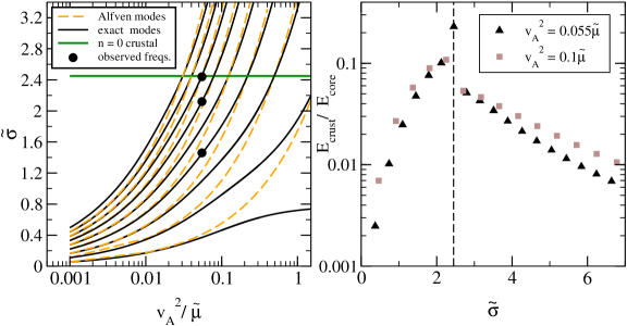
Figure 1: Left panel: A part of the global mode spectrum for the toy model of a magnetar with crust-core coupling, see text for details. The data corresponds to $\ell=2$ and $\Delta=0.1R$. Note the triple intersection between the exact mode solution from eqn. (14), the Alfvén modes from eqn. (16), and the fundamental crustal frequency $\tilde{\sigma}_{0}=2.45$. The black dots correspond to observed QPOs frequencies for SGR 1806-20, see text for discussion. Right panel: Assessing the excitation of various modes by means of the ratio between the mode energy in the crust $E_{\rm crust}$ and that in the core, $E_{\rm core}$. The dashed line labels the crustal frequency $\tilde{\sigma}_{0}$.

The coupled crust-core system obviously has a much richer set of oscillation modes than the decoupled elastic crust. Yet one can interpret most of the observed QPOs as pure crust modes for various values of $\ell$, see the discussion of Strohmayer & Watts (2005). At first sight our results may seem at variance with this interpretation. After all, our system has a number of additional modes. If they are not observed we need to explain why. To do this, we take the standard model for the giant flares at face value. The magnetic field erupts and induces a starquake in the crust. On the grounds of physical intuition we would expect that the initial perturbation in the crust will predominantly excite those global modes which communicate the least amount of energy to the core. To test this idea, we calculate the total energy (kinetic + magnetic) associated with each mode and consider the ratio $E_{\rm crust}/E_{\rm core}$. As can be seen from the right panel of Fig. 1, the results corroborate our intuition. The mode which maximises the energy ratio, i.e. should be easier to excite from an initial crust motion, is the one nearest to the resonant frequency $\sigma_{\rm A}=\sigma_{0}$ (analogous behaviour to that depicted in the right panel of Fig. 1 is found for modes in the vicinity of all higher $\sigma_{n}$ frequencies, for any $\ell$). This would explain why the other modes of the system are more difficult to excite, they are predominantly core-Alfvén modes which would be energetically more expensive to excite via the proposed mechanism. Similar conclusions can be drawn from the displacement $\xi^{x}$, displayed in Fig. 2, for a fixed value of $v_{\rm A}^{2}/{\tilde{\mu}}$, as we move upwards in the spectrum. The oscillation amplitude is generally far greater in the core, but the modes located in the vicinity of the crust frequencies $\sigma_{n}$ are exceptions. In those cases the crust oscillates with a comparable amplitude. However, these modes cannot be considered as “crustal”. The eigenfunctions clearly show that they represent global oscillations.

The conclusion of this discussion is that once the crust is shaken by a starquake the core-crust system will naturally choose to vibrate in those global modes which have frequencies similar to the frequencies of the toroidal modes of the uncoupled crust, with identical values of $\ell$ (and number of nodes in the crust). Hence, the model provides an explanation for all observed QPO frequencies, both intermediate ($\sim 30-155~{}$ Hz, different values of $\ell$) and high frequency ($\sim 625~{}$ Hz, overtone with one node in the crust). Our model differs from previous ones only in that the modes are global, not localised to the crust, and hence have a significant amplitude in the core.

A key feature of Figure 1 is the existence of modes with frequencies below the fundamental crustal frequency $\sigma_{0}$. This is interesting since the presence of low frequency QPOs has been confirmed in the data of both the RXTE and RHESSI satellites (Israel et al, 2005; Watts & Strohmayer, 2006): $18,26~{}$ and $30$ Hz QPOs for the December 2004 giant flare in SGR 1806-20. It is natural to identify the 30 Hz QPO with the fundamental crustal frequency $\sigma_{0}$ (Israel et al, 2005), since the higher frequency QPOs then fit the predictions from Eq. (2) quite well. However, we then find ourselves left with a puzzle: what is the origin of the remaining two frequencies? There are certainly no toroidal crustal modes with frequency below $\sigma_{0}$. Our model offers a natural explanation for these low-frequency modes.

Although our model is not designed to provide us with quantitatively accurate predictions, we can still attempt to match the observed data for the low frequency QPOs of SGR 1806-20. To do this we first identify $\tilde{\sigma}_{0}=2.45$ with the $30$ Hz frequency (presumably, this identification can be made rigorous in a calculation for a realistic neutron star model). Then the frequencies $18$ and $26$ Hz correspond to modes with $\tilde{\sigma}=1.46$ and $2.12$, respectively. Some navigation in Fig. 1 leads us to the value $v_{\rm A}^{2}=0.055{\tilde{\mu}}$ which has all three desired modes (indicated by filled circles in the figure). This value is reasonably consistent with $B_{15}\approx 1$ assuming $\rho_{14}\approx 1$ (note that the magnetic field estimated from the spin-down rate for SGR 1806-20 is $7.8\times 10^{14}$ G (Woods & Thompson, 2004). Moreover, the energy argument indicates that it is reasonable to expect these QPOs to be excited, cf. Fig. 1. Finally, we have an additional mode at $\approx 22$ Hz. In a sense, this could be considered a testable prediction. It would certainly be rewarding if a QPO with this intermediate frequency were to be found in the data!

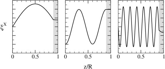
Figure 2: Fluid displacement $\xi^{x}$ for $\ell=2,~{}\Delta=0.1R$ and $v_{\rm A}^{2}=0.055\,{\tilde{\mu}}$. The modes illustrated are, from left to right: $\tilde{\sigma}=0.74,2.45,9.87$. In the middle panel note the comparable oscillation amplitudes in the crust and the core for the mode with $\sigma\approx\sigma_{0}=\sigma_{\rm A}$.

4 Concluding remarks

We have used a simple plane-parallel toy-model to discuss global MHD modes of a neutron star. The model, which takes into account the magnetic coupling between the elastic crust and the fluid core, provides results that are highly suggestive. The system is characterised by a rich spectrum of global modes “living” both in the crust and core, with a mixed magneto-elastic identity. Among myriads of available modes (for a given multipole $\ell$ and ratio of Alfvén velocity to shear velocity) the system will naturally excite the mode(s) which transfer as little energy as possible to the core, thus minimising the overall energy budget. We demonstrated that these favoured global oscillation modes have frequencies that are similar to the “pure crustal” frequencies from the non-magnetic problem. Our model provides support for the asteroseismology interpretation for the observed magnetar QPOs. In addition, it provides a natural explanation for the presence of lower frequency ($<30$ Hz) QPOs seen in the December 2004 giant flare of SGR 1806-20.

Even though our model is based on drastic simplifications, the basic physics predicted should survive for more realistic neutron star models. Obviously, one must expect corrections (and extra technical complications!) once the real problem is considered. A more complex magnetic field configuration will lead to intricate coupling between different multipoles, non-uniform density/crust elasticity and core stratification leading to buoyancy effects are likely to affect the mode structure, and the expected superconductivity will affect that nature of the Alfven waves. Nevertheless, global MHD modes due to the inescapable crust-core coupling are still likely to emerge, leading to intricate resonance phenomena.

References

- Abney et al (1996) Abney M., Epstein R.I., and Olinto A., 1996, ApJ, 466, L91
- Barat et al (1983) Barat C. et al, 1983, A & A, 126, 400
- Carroll et al (1986) Carroll B.W. et al, 1986, ApJ, 305, 767
- Douchin & Haensel (2001) Douchin F. and Haensel P., 2001, A & A, 380, 151
- Duncan & Thompson (1992) Duncan R.C. and Thompson C., 1992, ApJ, 392, L9
- Duncan (1998) Duncan R.C., 1998, ApJ, 498, L45
- Easson (1979) Easson I., 1979, ApJ, 228, 257
- Hansen & Cioffi (1980) Hansen C.J. and Cioffi D.F., 1980, ApJ, 238, 740
- Israel et al (2005) Israel G.L. et al, 2005, ApJ, 628, L53
- Levin (2006) Levin Y., 2006, MNRAS, 368, L35
- McDermott et al (1988) McDermott P.N., Van Horn H.M., and Hansen C.J., 1988, ApJ, 325, 725
- Messios et al (2001) Messios N., Papadopoulos D.M., and Stergioulas N., 2001, MNRAS, 328, 1161
- Piro (2005) Piro A.L., 2005, ApJ, 634, L153
- Strohmayer (1991) Strohmayer T.E., 1991, ApJ, 372, 573
- Strohmayer & Watts (2005) Strohmayer T.E., and Watts A.L., 2005, ApJ, 632, L111
- Thomson & Duncan (1995) Thomson C., and Duncan R.C., 1995, MNRAS, 275, 255
- Van Horn (1980) Van Horn H.M., 1980, ApJ, 236, 899
- Watts & Strohmayer (2006) Watts A.L., and Strohmayer T.E., 2006, ApJ, 637, L117
- Woods & Thompson (2004) Woods P.M., and Thompson C., 2004, in “Compact Stellar X-ray Sources” eds. W.H.G. Lewin and M. Van der Klis (preprint astro-ph/0406133)