Evolution of magnetized, differentially rotating neutron stars: Simulations in full general relativity

Abstract

We study the effects of magnetic fields on the evolution of differentially rotating neutron stars, which can be formed in stellar core collapse or binary neutron star coalescence. Magnetic braking and the magnetorotational instability (MRI) both act on differentially rotating stars to redistribute angular momentum. Simulations of these stars are carried out in axisymmetry using our recently developed codes which integrate the coupled Einstein-Maxwell-MHD equations. We consider stars with two different equations of state (EOS), a gamma-law EOS with $\Gamma=2$, and a more realistic hybrid EOS, and we evolve them adiabatically. Our simulations show that the fate of the star depends on its mass and spin. For initial data, we consider three categories of differentially rotating, equilibrium configurations, which we label normal, hypermassive and ultraspinning. Normal configurations have rest masses below the maximum achievable with uniform rotation, and angular momentum below the maximum for uniform rotation at the same rest mass. Hypermassive stars have rest masses exceeding the mass limit for uniform rotation. Ultraspinning stars are not hypermassive, but have angular momentum exceeding the maximum for uniform rotation at the same rest mass. We show that a normal star will evolve to a uniformly rotating equilibrium configuration. An ultraspinning star evolves to an equilibrium state consisting of a nearly uniformly rotating central core, surrounded by a differentially rotating torus with constant angular velocity along magnetic field lines, so that differential rotation ceases to wind the magnetic field. In addition, the final state is stable against the MRI, although it has differential rotation. For a hypermassive neutron star, the MHD-driven angular momentum transport leads to catastrophic collapse of the core. The resulting rotating black hole is surrounded by a hot, massive, magnetized torus undergoing quasistationary accretion, and a magnetic field collimated along the spin axis—a promising candidate for the central engine of a short gamma-ray burst.

I Introduction

Differentially rotating neutron stars can form from the collapse of massive stellar cores, which likely acquire rapid differential rotation during collapse even if they are spinning uniformly at the outset zm97 ; diffrot (see also liu01 ). Differential rotation can also arise from the mergers of binary neutron stars RS99 ; SU00 ; FR00 . In these new-born, dynamically stable, neutron stars, magnetic fields and/or viscosity will transport angular momentum and cause a substantial change in the configurations on a secular timescale.

Some newly-formed differentially rotating neutron stars may be hypermassive. Specifically, the mass limits for non-rotating stars [the Oppenheimer-Volkoff limit] and for rigidly rotating stars (the supramassive limit, which is only about 20% larger) can be significantly exceeded by the presence of differential rotation BSS ; MBS04 . Mergers of binary neutron stars could lead to the formation of such hypermassive neutron stars (HMNSs) as remnants. This possibility was foreshadowed in Newtonian RS99 , post-Newtonian FR00 , and in full general relativistic simulations SU00 . The latest binary neutron star merger simulations in full general relativity STUa ; STUb ; STUc have confirmed that HMNS formation is indeed a possible outcome. HMNSs could also result from core collapse of massive stars.

Differentially rotating stars tend to approach rigid rotation when acted upon by processes which transport angular momentum. HMNSs, however, cannot settle down to rigidly rotating neutron stars since their masses exceed the maximum allowed by rigid rotation. Thus, delayed collapse to a black hole and, possibly, mass loss may result after sufficient transport of angular momentum from the inner to the outer regions. Several processes can act to transport angular momentum and drive the HMNS to collapse. Previous calculations in full general relativity have modeled the evolution of HMNS driven by viscous angular momentum transport DLSS and by angular momentum loss due to gravitational radiation STUb . In both cases, the core of the HMNS eventually collapses to a black hole. However, in the case of viscosity-driven evolution, a large accretion torus is found to develop around the newly-formed black hole, while for gravitational wave-driven evolution, the disk present after collapse is very small. The size of the disk is of crucial importance, because if a large disk is produced, the post-collapse system may produce a short-duration gamma-ray burst (GRB).

The merger of binary neutron stars has been proposed for many years as an explanation of short-hard GRBs GRB ; GRB-BNS . Possible associations between short GRBs and elliptical galaxies reported recently short make it unlikely that short GRBs are related to supernova stellar core collapse. The merger of compact-object binaries (neutron star-neutron star or black hole-neutron star) is now the favored hypothesis for explaining short GRBs. According to this scenario, after the merger, a stellar-mass black hole is formed, surrounded by hot accretion torus containing $\sim 1$–$10\%$ of the total mass of the system. Energy extracted from this system, either by MHD processes or neutrino-radiation, powers the fireball for the GRB. The viability of this model depends on the presence of a significantly massive accretion disk after the collapse of the remnant core, which in turn depends on the mechanism driving the collapse.

Though magnetic fields likely play a significant role in the evolution of HMNSs, the numerical tools needed to study this problem have not been available until recently. In particular, the evolution of magnetized HMNSs can only be determined by solving the coupled Einstein-Maxwell-MHD equations self-consistently in full general relativity. Recently, Duez et al. DLSS2 and Shibata and Sekiguchi SS independently developed codes designed to do such calculations for the first time (see also valencia:fn ). The first simulations of magnetized hypermassive neutron star collapse (assuming both axial and equatorial symmetry) were reported in DLSSS1 , and the implications of these results for short GRBs were presented in GRB2 . These simulations proved that the amplification of small seed magnetic fields by a combination of magnetic winding and the magnetorotational instability (MRI) is sufficient to trigger collapse in hypermassive stars on the Alfvén timescale, confirming earlier predictions BSS ; Shapiro . In the present work, we describe these collapse calculations in more detail.

We also compare the results for hypermassive stars with the evolution of two differentially rotating models below the supramassive limit in order to highlight the qualitatively different physical effects which arise in the evolution. Given a fixed equation of state (EOS), the sequence of uniformly rotating stars with a given rest mass has a maximum angular momentum $J_{\rm max}$. A nonhypermassive star having angular momentum $J>J_{\rm max}$ is referred to as an “ultraspinning” star. We perform simulations on the MHD evolution of two nonhypermassive stars – one is ultraspinning and the other is not; we refer to the later as “normal.” Instead of collapsing, they settle down to a new equilibrium state after several Alfvén times. The normal star settles down to a uniformly rotating configuration. In contrast, the ultraspinning star settles down to a nearly uniformly rotating central core, surrounded by a differentially rotating torus. In this new equilibrium, the system has adjusted to a state where the angular velocity is constant along the magnetic field lines, which means that the residual differential rotation ceases further magnetic winding. In addition, we find that the final state is also stable against the MRI, although it has differential rotation.

The key subtlety in all of these simulations is that the wavelengths of the MRI modes must be well resolved on the computational grid. Since this wavelength is proportional to the magnetic field strength, it becomes very difficult to resolve for small seed fields. However, the simulations reported here succeed in resolving the MRI.

The structure of this paper is as follows. We give an overview of the MHD effects acting on differentially rotating stars in Sec. II. The initial models are briefly discussed in Sec. III. In Sec. IV we summarize the set of coupled Einstein-Maxwell-MHD equations which are solved during the simulations. We outline our numerical methods for the evolution in Sec. V, and present our simulation results in Sec. VI. Finally, we summarize and discuss our main results in Sec. VII. In what follows, we assume geometrized units such that $G=c=1$.

II Overview of MHD effects

Two distinct processes which are known to transport angular momentum in differentially rotating magnetized fluids are magnetic braking spitzer ; spruit ; BSS ; Shapiro and the MRI MRI0 ; MRI . Magnetic braking transports angular momentum on the Alfvén time scale BSS ; Shapiro :

$$t_{A}\sim\frac{R}{v_{A}}\sim 10^{2}~{}{\rm s}\left(\frac{B}{10^{12}~{}{\rm G}}\right)^{-1}\left(\frac{R}{15~{}{\rm km}}\right)^{-1/2}\left(\frac{M}{3M_{\odot}}\right)^{1/2}\ ,$$ (1)

where $R$ is the radius of the HMNS and $v_{A}$ is the Alfvén speed.

At early times, the effects of magnetic braking grow linearly with time. This can be seen by considering the magnetic induction equation in a perfectly conducting (MHD) plasma [see Eq. (38) below]:

$$\partial_{t}\tilde{B}^{i}+\partial_{j}(v^{j}\tilde{B}^{i}-v^{i}\tilde{B}^{j})=0\ ,$$ (2)

where

$$\tilde{B}^{i}\equiv\sqrt{\gamma}B^{i}=\sqrt{\gamma}n_{\nu}F^{*\nu i}\ .$$ (3)

In the above formulae, $\gamma$ is the determinant of the spatial metric, $n_{\mu}=(-\alpha,0,0,0)$ is the normal to the spatial hypersurface, $\alpha$ is the lapse, $F^{*\mu\nu}$ is the dual of the Faraday tensor, and $v^{i}=u^{i}/u^{0}$ is the 3-velocity of the fluid. Now, if the magnetic field is weak and has a negligible backreaction on the fluid, the velocities will remain constant with time. In cylindrical coordinates, we have (assuming axisymmetry)

$$\partial_{t}\tilde{B}^{i} \approx 0\ ,\ \ \ \ \ \ \ \ \ \ \ \ \ \ \ \ \ (i=\varpi,z)$$ (4)

$$\partial_{t}\tilde{B}^{\varphi} = -\partial_{i}(v^{i}\tilde{B}^{\varphi}-v^{\varphi}\tilde{B}^{i})$$ (5)

$$\approx \partial_{i}(v^{\varphi}\tilde{B}^{i})\ ,\ \ \ \ \ \ \ (i=\varpi,z)$$

where $\varpi$ is the cylindrical radius, and where we have used the fact that $v^{\varpi}=v^{z}=0$ at $t=0$ and remains so under these assumptions. Then, since $v^{\varphi}=\Omega$ (the angular velocity),

$$\partial_{t}\tilde{B}^{\varphi}\approx\tilde{B}^{i}\partial_{i}\Omega+\Omega\partial_{i}\tilde{B}^{i}\ \ \ \ \ (i=\varpi,z).$$ (6)

The second term vanishes by Maxwell’s equations (the no-monopole constraint, $\partial_{i}\tilde{B}^{i}=0$) and the assumption of axisymmetry ($\partial_{\varphi}=0$). At early times, Eq. (6) indicates that the toroidal component of the field $B^{T}\equiv\varpi B^{\varphi}$ grows linearly according to

$$B^{T}(t;\varpi,z)\approx t\varpi B^{i}(0;\varpi,z)\partial_{i}\Omega(0;\varpi,z)\ \ \ \ \ (i=\varpi,z)\ .$$ (7)

The growth of $B^{T}$ is expected to deviate from this linear relation when the tension due to the winding up of magnetic field lines begins to change the angular velocity profile of the fluid.

The MRI is present in a weakly magnetized, rotating fluid wherever $\partial_{\varpi}\Omega<0$ MRI ; MRIrev . When the instability reaches the nonlinear regime, the distortions in the magnetic field lines and velocity field lead to turbulence. To estimate the growth timescale $t_{\rm MRI}$ and the wavelength of the fastest growing mode $\lambda_{\rm max}$, we make use of a simple Newtonian linear analysis given in MRIrev (see also gammie04 ). Linearizing the MHD equations for a local patch of a rotating fluid and imposing $e^{i({\bf k}\cdot{\bf x}-\omega t)}$ dependence on the perturbations leads to the dispersion relation given in Eq. (125) of MRIrev . Specializing this equation for a constant entropy star and considering only modes in the vertical direction, this reduces to

$$\omega^{4}-[2({\bf k}\cdot{\bf v}_{A})^{2}+\kappa^{2}]\omega^{2}+({\bf k}\cdot{\bf v}_{A})^{2}[({\bf k}\cdot{\bf v}_{A})^{2}+\kappa^{2}-4\Omega^{2}]=0\ ,$$ (8)

where ${\bf v}_{A}={\bf B}/\sqrt{4\pi\rho}$ is the (Newtonian) Alfvén velocity, $\rho$ is the mass density and $\kappa$ is the “epicyclic frequency” of Newtonian theory:

$$\kappa^{2}\equiv\frac{1}{r^{3}}\frac{\partial(r^{4}\Omega^{2})}{\partial r}=4\Omega^{2}+2\Omega\frac{\partial\Omega}{\partial\ln r}\ .$$ (9)

We consider vertical modes (${\bf k}=k{\bf e}_{z}$) since we are only looking for an estimate of $\lambda_{\rm max}$, and since these are likely to be the dominant modes.

Since the dispersion relation in Eq. (8) is quadratic in $\omega^{2}$, it can be easily solved for $\omega^{2}$ and then minimized to find the frequency of the fastest-growing mode, $\omega_{\rm max}$:

$$-\omega^{2}_{\rm max}=\frac{s^{4}}{4(s^{2}+\kappa^{2})}=\frac{1}{4}\left(\frac{\partial\Omega}{\partial\ln r}\right)^{2}\ ,$$ (10)

where $s^{2}=4\Omega^{2}-\kappa^{2}=-2\Omega\partial\Omega/\partial\ln r$. This maximum growth rate corresponds to

$$({\bf k}\cdot{\bf v}_{A})^{2}_{\max}=\frac{s^{2}}{4}\left(\frac{s^{2}+2\kappa^{2}}{s^{2}+\kappa^{2}}\right)\ .$$ (11)

For the growth time and wavelength of the fastest growing mode, we then have

$$t_{\rm MRI} = 2\left(\partial\Omega/\partial\ln\varpi\right)^{-1}\ ,$$ (12)

$$\lambda_{\rm max} = \frac{4\pi v_{A}^{z}}{s}\sqrt{\frac{s^{2}+\kappa^{2}}{s^{2}+2\kappa^{2}}}\ .$$ (13)

In order of magnitude,

$$\lambda_{\rm max} \sim 2\pi v_{A}^{z}/\Omega$$ (14)

$$\sim 3~{}{\rm cm}\ \left(\frac{\Omega}{4000\ {\rm rad}\ {\rm s}^{-}1}\right)^{-1}\left(\frac{B}{10^{12}\ {\rm G}}\right)$$

$$t_{\rm MRI} \sim 1/\Omega\sim 0.25~{}{\rm ms}\ \left(\frac{\Omega}{4000\ {\rm rad}\ {\rm s}^{-}1}\right)^{-1}\ .$$ (15)

Here $\Omega=4000~{}{\rm rad}~{}{\rm s}^{-1}$ corresponds to a rotation period $P=1.57$ ms. For realistic HMNS magnetic fields, $\lambda_{\rm max}$ will be much smaller than $R$. We note that, since $\lambda_{\rm max}\propto v_{A}$, larger magnetic fields will result in longer MRI wavelengths. When $\lambda_{\rm max}\mathrel{\raise 1.29167pt\hbox{$>$}\mkern-14.0mu\lower 2.58334pt\hbox{$\sim$}}R$, where $R$ is the equatorial radius of the star, the MRI will be suppressed since the unstable perturbations will no longer fit inside the star. This is why the MRI is regarded as a weak-field instability. Typically, we set magnetic field amplitudes so that $\lambda_{\rm max}\sim R/10$ for the models we consider here. We note that $t_{\rm MRI}$ is independent of the strength of the seed magnetic field. The MRI always grows on a dynamical timescale for a sufficiently differentially rotating configuration. Hence, the MRI is likely to be very important during the early evolution for realistic HMNSs. However, the resulting angular momentum transport is governed by the turbulence and is thus expected to occur on a timescale longer than $t_{\rm MRI}$.

Magnetic fields and turbulence tend to transport specific angular momentum from the rapidly rotating inner region of a differentially rotating star to the more slowly rotating outer layers. This causes the inner part to contract and the outer layers to expand. Since hypermassive stars depend on their strong differential rotation for stability, this angular momentum transport process likely leads to collapse. However, in Section VI.3, we show that very different behavior can result for rapidly rotating nonhypermassive models. In the example we explore, the star readjusts to a new equilibrium state consisting of a nearly rigidly rotating core surrounded by a differentially rotating torus in which the magnetic field lines are everywhere orthogonal to the gradient of the angular velocity (i.e., $B^{j}\partial_{j}\Omega=0$). Hence, magnetic winding shuts down even though the configuration is still differentially rotating. This possibility has been discussed previously by Spruit spruit in the context of Newtonian theory.

III Initial Models

In order to study the effects of rotation and EOS, we evolve four representative differentially rotating stars, which we call “A”, “B1”, “B2” and “C”. Their properties are listed in Table 1. Stars A and C are hypermassive; stars B1 and B2 are not. These configurations are all dynamically stable.

Table 1: Initial Models

Case	EOS	$M_{0}/M_{0,\rm{TOV}}$a	$M_{0}/M_{0,\rm{sup}}$b	$M/M_{\rm sup}$c	$R_{\rm eq}/M$d	$J/M^{2}$${\ }^{\rm e}$	$T_{\rm rot}/|W|$f	$\Omega_{\rm eq}/\Omega_{c}$g	$P_{c}/M$h
A	$\Gamma=2$	1.69	1.46	1.49	4.48	1.0	0.249	0.33	38.4
B1	$\Gamma=2$	0.99	0.86	0.89	8.12	1.0	0.181	0.40	103
B2	$\Gamma=2$	0.98	0.85	0.86	4.84	0.38	0.040	0.34	105
C	hybrid	1.28	1.14	1.17	2.75	0.82	0.241	0.185	15.5

^a The ratio of the rest mass $M_{0}$ to the TOV rest mass limit for the given EOS.

^b The ratio of the rest mass $M_{0}$ to the rest mass limit for uniformly rotating stars of the given EOS (the supramassive limit). If this ratio is greater than unity, the star is hypermassive.

^c The ratio of the ADM mass $M$ to the gravitational mass limit for uniformly rotating stars of the given EOS.

^d The equatorial coordinate radius $R_{\rm eq}$ normalized by the ADM mass.

^e The ratio of the angular momentum $J$ to $M^{2}$ (the angular momentum parameter).

^f The ratio of the rotational kinetic energy to the gravitational binding energy [see Eqs. (58) and (60)].

^g The ratio of the angular velocity at the equator to the central angular velocity.

^h The initial central rotation period $P_{c}$ normalized by the ADM mass.

Stars A, B1 and B2 are constructed using a $\Gamma=2$ polytropic EOS, $P=K\rho_{0}^{\Gamma}$, where $P$, $K$, and $\rho_{0}$ are the pressure, polytropic constant, and rest-mass density, respectively. (In DLSS , which considered evolution with shear viscosity, star A was referred to as “star I” and star B1 was referred to as “star V”). The rest mass of star A exceeds the supramassive limit by 46%, while the rest masses of stars B1 and B2 are below the supramassive limit. The angular momentum of star B1 exceeds the maximum angular momentum ($J_{\rm max}$) for a rigidly rotating star with the same rest mass and EOS, whereas star B2 has angular momentum $J<J_{\rm max}$. Thus, star B1 is “ultraspinning,” while star B2 is “normal.” Stars A, B1 and B2 may be scaled to any desired physical mass by adjusting the value of $K$ CST . In general, $M\propto K^{n/2}$, where $n$ is the polytropic index ($\Gamma=1+1/n$, here $n=1$). For example, choosing $K=2.42\times 10^{5}{\rm g}^{-1}{\rm cm}^{5}{\rm s}^{-2}$ gives the maximum ADM mass (rest mass) of $2.12M_{\odot}$ ($2.32M_{\odot}$) for spherical neutron stars and $2.42M_{\odot}$ ($2.67M_{\odot}$) for rigidly rotating neutron stars.

In order to consider the effects of a more realistic neutron star equation of state, star C is constructed from a cold hybrid EOS zm97 ; SS defined as follows:

$$P=P_{\rm cold}=\left\{\begin{array}[]{ll}K_{1}\rho_{0}^{\Gamma_{1}}&\mbox{for $\rho_{0}\leq\rho_{\rm nuc}$}\\ K_{2}\rho_{0}^{\Gamma_{2}}&\mbox{for $\rho_{0}\geq\rho_{\rm nuc}$}\end{array}\right.\ .$$ (16)

We set $\Gamma_{1}=1.3$, $\Gamma_{2}=2.75$, $K_{1}=5.16\times 10^{14}$ cgs, $K_{2}=K_{1}\rho_{\rm nuc}^{\Gamma_{1}-\Gamma_{2}}$, and $\rho_{\rm nuc}=1.8\times 10^{14}~{}{\rm g/cm^{3}}$. With this EOS, the maximum ADM mass (rest mass) is $2.01M_{\odot}~{}(2.32M_{\odot})$ for spherical neutron stars and $2.27M_{\odot}~{}(2.60M_{\odot})$ for rigidly rotating neutron stars, which are similar values to those in realistic stiff EOSs EOS . Star C exceeds the supramassive limit by 14%. The various parameters of star C are chosen in order to more closely mimic the HMNSs formed through binary neutron star mergers with realistic equations of state in STUb .

Following previous papers (e.g, CST ; BSS ; SBS ; DLSS ), we choose the initial rotation law $u^{0}u_{\varphi}=A^{2}(\Omega_{c}-\Omega)$, where $u^{\mu}$ is the four-velocity, $\Omega_{c}$ is the angular velocity along the rotational axis, and $\Omega\equiv u^{\varphi}/u^{0}$ is the angular velocity. In the Newtonian limit, this rotation law becomes

$$\Omega=\frac{\Omega_{c}}{1+{\frac{\varpi^{2}}{A^{2}}}}\ .$$ (17)

The constant $A$ has units of length and determines the steepness of the differential rotation. In this paper, $A$ is set equal to the coordinate equatorial radius $R_{\rm eq}$ for stars A, B1, and B2, while $A=0.8R_{\rm eq}$ for star C. The corresponding values of $\Omega_{\rm eq}/\Omega_{c}$ are shown in Table 1 (where $\Omega_{\rm eq}$ is the angular velocity at the equatorial surface). The magnitude of the angular momentum is seen from the Kerr parameter $a/M=q\equiv J/M^{2}$. Stars A, B1, and C have $q=$ 1.0, 1.0, and 0.82, respectively. These stars rotate very rapidly and are highly flattened due to centrifugal force. Star B2, on the other hand, has a comparatively low angular momentum parameter: $q=0.38$.

We must also specify initial conditions for the magnetic field. We choose to add a weak poloidal magnetic field to the equilibrium model by introducing a vector potential of the following form $A_{\varphi}=\varpi^{2}{\rm max}[A_{b}(P-P_{\rm cut}),0]$, where the cutoff $P_{\rm cut}$ is 4% of the maximum pressure, and $A_{b}$ is a constant which determines the initial strength of the magnetic field. We characterize the strength of the initial magnetic field by $C\equiv{\rm max}(b^{2}/P)$, i.e. the maximum value on the grid of the ratio of the magnetic energy density to the pressure. We choose $A_{b}$ such that $C\sim 10^{-3}$–$10^{-2}$. We have verified that such small initial magnetic fields introduce negligible violations of the Hamiltonian and momentum constraints in the initial data.

IV Basic Equations

IV.1 Evolution of the gravitational fields

We evolve the 3-metric $\gamma_{ij}$ and extrinsic curvature $K_{ij}$ using the Baumgarte-Shapiro-Shibata-Nakamura (BSSN) formulation BSSN . The fundamental variables for BSSN evolution are

$$\phi \equiv {1\over 12}\ln[\det(\gamma_{ij})]\ ,$$ (18)

$$\tilde{\gamma}_{ij} \equiv e^{-4\phi}\gamma_{ij}\ ,$$ (19)

$$K \equiv \gamma^{ij}K_{ij}\ ,$$ (20)

$$\tilde{A}_{ij} \equiv e^{-4\phi}(K_{ij}-{1\over 3}\gamma_{ij}K)\ ,$$ (21)

$$\tilde{\Gamma}^{i} \equiv -\tilde{\gamma}^{ij}{}_{,j}\ \ \ ({\rm or}~{}~{}F_{i}\equiv\delta^{jk}\tilde{\gamma}_{ij,k})\ .$$ (22)

The evolution equations for these variables are as follows:

$$(\partial_{t}-{\mathcal{L}}_{\beta})\tilde{\gamma}_{ij} = -2\alpha\tilde{A}_{ij}$$ (23)

$$(\partial_{t}-{\mathcal{L}}_{\beta})\phi = -{1\over 6}\alpha K$$ (24)

$$(\partial_{t}-{\mathcal{L}}_{\beta})K = -\gamma^{ij}D_{j}D_{i}\alpha+{1\over 3}\alpha K^{2}$$

$$+\alpha\tilde{A}_{ij}\tilde{A}^{ij}+4\pi\alpha(\rho+S)$$

$$(\partial_{t}-{\mathcal{L}}_{\beta})\tilde{A}_{ij} = e^{-4\phi}(-D_{i}D_{j}\alpha+\alpha(R_{ij}-8\pi S_{ij}))^{TF}$$ (26)

$$+\alpha(K\tilde{A}_{ij}-2\tilde{A}_{il}\tilde{A}^{l}{}_{j})\ ,$$

where $\alpha$ is the lapse function, $\beta^{i}$ is the shift, ${\mathcal{L}}_{\beta}$ is the Lie derivative along the shift, and $D_{i}$ is the covariant derivative with respect to the spatial 3-metric. The Ricci tensor $R_{ij}$ can be written as the sum

$$R_{ij}=\tilde{R}_{ij}+R_{ij}^{\phi}.$$ (27)

Here $R_{ij}^{\phi}$ is

$$R^{\phi}_{ij} = -2\tilde{D}_{i}\tilde{D}_{j}\phi-2\tilde{\gamma}_{ij}\tilde{D}^{l}\tilde{D}_{l}\phi$$ (28)

$$+4(\tilde{D}_{i}\phi)(\tilde{D}_{j}\phi)-4\tilde{\gamma}_{ij}(\tilde{D}^{l}\phi)(\tilde{D}_{l}\phi),$$

where $\tilde{D}^{i}=\tilde{\gamma}^{ij}\tilde{D}_{j}$. The “tilde” Ricci tensor $\tilde{R}_{ij}$ is the Ricci tensor associated with $\tilde{\gamma}_{ij}$, and is computed by

$$\tilde{R}_{ij} = -\frac{1}{2}\tilde{\gamma}^{lm}\tilde{\gamma}_{ij,lm}+\tilde{\gamma}_{k(i}\partial_{j)}\tilde{\Gamma}^{k}+\tilde{\Gamma}^{k}\tilde{\Gamma}_{(ij)k}+$$ (29)

$$\tilde{\gamma}^{lm}\left(2\tilde{\Gamma}^{k}_{l(i}\tilde{\Gamma}_{j)km}+\tilde{\Gamma}^{k}_{im}\tilde{\Gamma}_{klj}\right)\ ,$$

where

$$\tilde{\Gamma}_{ijk}=\frac{1}{2}(\tilde{\gamma}_{ij,k}+\tilde{\gamma}_{ik,j}-\tilde{\gamma}_{jk,i})\ .$$ (30)

The evolution of $\tilde{\Gamma}^{i}$ is given by

$$\partial_{t}\tilde{\Gamma}^{i} = \partial_{j}(2\alpha\tilde{A}^{ij}+{\mathcal{L}}_{\beta}\tilde{\gamma}^{ij})$$

$$= \tilde{\gamma}^{jk}\beta^{i}{}_{,jk}+{1\over 3}\tilde{\gamma}^{ij}\beta^{k}{}_{,kj}-\tilde{\Gamma}^{j}\beta^{i}{}_{,j}$$

$$+{2\over 3}\tilde{\Gamma}^{i}\beta^{j}{}_{,j}+\beta^{j}\tilde{\Gamma}^{i}{}_{,j}-2\tilde{A}^{ij}\partial_{j}\alpha$$

$$-2\alpha\left({2\over 3}\tilde{\gamma}^{ij}K_{,j}-6\tilde{A}^{ij}\phi_{,j}-\tilde{\Gamma}^{i}{}_{jk}\tilde{A}^{jk}+8\pi\tilde{\gamma}^{ij}S_{j}\right)\ .$$

The matter source terms $\rho$, $S_{ij}$, $S_{i}$ and $S$ are related to the stress-energy tensor $T^{\mu\nu}$ as follows:

$$\rho = n_{\alpha}n_{\beta}T^{\alpha\beta}\ ,$$

$$S_{i} = -\gamma_{i\alpha}n_{\beta}T^{\alpha\beta}\ ,$$

$$S_{ij} = \gamma_{i\alpha}\gamma_{j\beta}T^{\alpha\beta}\ ,$$

$$S = S^{i}{}_{i}\ .$$ (32)

In the code of Duez et al. DLSS2 , additional constraint damping terms are included in the BSSN evolution system, as described in ybs02 ; excision (see Eqs. (45) and (46) of ybs02 , Eqs. (6)–(8), (11), (13) and (15) of excision ). The gauge conditions used with this code are the following hyperbolic driver conditions abpst01 ; excision :

$$\partial_{t}\alpha = \alpha{\cal A}\ ,$$

$$\partial_{t}{\cal A} = -a_{1}(\alpha\partial_{t}K+a_{2}\partial_{t}\alpha+a_{3}e^{-4\phi}\alpha K)\ ,$$ (33)

$$\partial^{2}_{t}\beta^{i} = b_{1}(\alpha\partial_{t}\tilde{\Gamma}^{i}-b_{2}\partial_{t}\beta^{i})\ ,$$ (34)

where $a_{1}$, $a_{2}$, $a_{3}$, $b_{1}$, and $b_{2}$ are freely specifiable constants. We usually choose $a_{1}=0.75$, $b_{1}=0.15$, $a_{2}$ and $b_{2}$ between $0.34/M$ and $0.56/M$, and $a_{3}$ between $0.17/M$ and $0.28/M$, where $M$ is the ADM mass of the star. For runs with excision, we use $a_{1}=b_{1}=0.75$, $a_{3}=0$, $0.34/M\leq a_{2}\leq 0.56/M$ and $b_{2}=a_{2}$.

In the code of Shibata and Sekiguchi SS the following dynamical gauge conditions are used:

$$\partial_{t}\alpha = -\alpha K,$$ (35)

$$\partial_{t}\beta^{i} = \tilde{\gamma}^{ij}(F_{j}+\Delta t\partial_{t}F_{j}),$$ (36)

where $\Delta t$ is the timestep, and $F_{i}$ is the function defined in Eq. (22). For the evolution, constraint damping terms are added to the equations for $\phi$ and $\tilde{A}_{ij}$ to suppress high-frequency noise and maintain the accuracy of the Hamiltonian constraint and tr$(\tilde{A}_{ij})=0$.

IV.2 Evolution of the electromagnetic fields

The evolution equation for the magnetic field in a perfectly conducting MHD fluid ($F^{\mu\nu}u_{\nu}=0$) can be obtained in conservative form by taking the dual of Maxwell’s equation $F_{[\mu\nu,\lambda]}=0$. One finds

$$\nabla_{\nu}F^{*\mu\nu}=\frac{1}{\sqrt{-g}}\partial_{\nu}(\sqrt{-g}\,F^{*\mu\nu})=0\ ,$$ (37)

where $\sqrt{-g}=\alpha\sqrt{\gamma}$, $F^{\alpha\beta}$ is the Faraday tensor, and $F^{*\alpha\beta}$ is its dual. Using the fact that the magnetic field as measured by a normal observer $n^{a}$ is given by $B^{i}=n_{\mu}F^{*\mu i}$, the time component of Eq. (37) gives the no-monopole constraint $\partial_{j}\tilde{B}^{j}=0$, where $\tilde{B}^{j}=\sqrt{\gamma}\,B^{j}$. The spatial components of Eq. (37) give the magnetic induction equation, which can be written as

$$\partial_{t}\tilde{B}^{i}+\partial_{j}(v^{j}\tilde{B}^{i}-v^{i}\tilde{B}^{j})=0\ .$$ (38)

IV.3 Evolution of the hydrodynamics fields

The evolution equations for the fluid are as follows DLSS2 ; SS :

$$\partial_{t}\rho_{*}+\partial_{j}(\rho_{*}v^{j}) = 0\ ,$$ (39)

$$\partial_{t}\tilde{S}_{i}+\partial_{j}(\alpha\sqrt{\gamma}\,T^{j}{}_{i}) = \frac{1}{2}\alpha\sqrt{\gamma}\,T^{\alpha\beta}g_{\alpha\beta,i}\ ,$$ (40)

$$\partial_{t}\tilde{\tau}+\partial_{i}(\alpha^{2}\sqrt{\gamma}\,T^{0i}-\rho_{*}v^{i}) = s\ ,$$ (41)

where the density variable is $\rho_{*}=\alpha\sqrt{\gamma}\rho_{0}u^{0}$, the momentum-density variable is $\tilde{S}_{i}=\alpha\sqrt{\gamma}T^{0}_{i}$, the energy-density variable as adopted by Duez et al. DLSS2 is $\tilde{\tau}=\alpha^{2}\sqrt{\gamma}\,T^{00}-\rho_{*}$, and the source term $s$ is

$$s = -\alpha\sqrt{\gamma}\,T^{\mu\nu}\nabla_{\nu}n_{\mu}$$ (42)

$$= \alpha\sqrt{\gamma}\,[(T^{00}\beta^{i}\beta^{j}+2T^{0i}\beta^{j}+T^{ij})K_{ij}$$ (44)

$$-(T^{00}\beta^{i}+T^{0i})\partial_{i}\alpha]\ .$$

The MHD stress-energy tensor is given by

$$T^{\mu\nu}=(\rho_{0}h+b^{2})u^{\mu}u^{\nu}+(P+b^{2}/2)g^{\mu\nu}-b^{\mu}b^{\nu}\ ,$$ (45)

where $b^{\mu}\equiv u_{\nu}F^{*\nu\mu}/\sqrt{4\pi}$, the specific enthalpy is given by $h\equiv 1+\epsilon+P/\rho_{0}$, $\epsilon$ is the specific internal energy, and $b^{2}=b_{\mu}b^{\mu}$.

In the code of Shibata and Sekiguchi SS , the energy evolution variable is chosen to be $\sqrt{\gamma}\,n_{\mu}n_{\nu}T^{\mu\nu}=\tilde{\tau}+\rho_{*}$, and the evolution equation may be obtained by adding Eq. (39) to Eq. (41).

The MHD system of equations is completed by a choice of EOS for the evolution. For stars A, B2, and B2, we adopt a $\Gamma$-law EOS $P=(\Gamma-1)\rho_{0}\epsilon$, with $\Gamma=2$. For star C, we adopt the following hybrid EOS:

$$P=P_{\rm cold}+(\Gamma_{\rm th}-1)\rho_{0}(\varepsilon-\varepsilon_{\rm cold}).$$ (46)

Here, $P_{\rm cold}$ and $\varepsilon_{\rm cold}$ denote the cold component of $P$ and $\varepsilon$ SS . The conversion efficiency of kinetic energy to thermal energy at shocks is determined by $\Gamma_{\rm th}$, which we set to 1.3 to conservatively account for shock heating.

IV.4 Diagnostics

We monitor several global conserved quantities to check the accuracy of our simulations. The ADM mass $M$ and angular momentum $J$ are defined as integrals over surfaces at infinity as follows integrals :

$$M = {1\over 16\pi}\int_{r=\infty}\sqrt{\gamma}\gamma^{im}\gamma^{jn}(\gamma_{mn,j}-\gamma_{jn,m})d^{2}S_{i}\ ,$$ (47)

$$J_{i} = {{1}\over{8\pi}}\varepsilon_{ij}{}^{k}\int_{r=\infty}x^{j}K_{k}^{m}d^{2}S_{m}\ .$$ (48)

In cases for which no singularity is present on the grid, these surface integrals can be converted to volume integrals using Gauss’s theorem (see Appendix A of ybs02 ):

$$M = \int_{V}\left[e^{5\phi}(\rho_{0}+{1\over 16\pi}\tilde{A}_{ij}\tilde{A}^{ij}-{1\over 24\pi}K^{2})\right.$$

$$\left.\quad-{1\over 16\pi}\tilde{\Gamma}^{ijk}\tilde{\Gamma}_{jik}+{1-e^{\phi}\over 16\pi}\tilde{R}\right]d^{3}x$$

$$J_{i} = \varepsilon_{ij}{}^{k}\int_{V}\Bigl{(}{1\over 8\pi}\tilde{A}^{j}_{k}+x^{j}S_{k}$$

$$\quad+{1\over 12\pi}x^{j}K_{,k}-{1\over 16\pi}x^{j}\tilde{\gamma}^{lm}{}_{,k}\tilde{A}_{lm}\Bigr{)}e^{6\phi}d^{3}x\ .$$

These integrals should be exactly conserved. However, using finite grids, we are unable to perform this integral out to infinity, and we expect to see mass and angular momentum losses due to outflows (of fluid, electromagnetic fields, and/or gravitational waves) through the boundaries. These fluxes can be measured, however, and are found to be quite small.

In axisymmetry, the volume integral for the angular momentum (which is entirely in the $z$-direction) simplifies considerably Wald :

$$J=\int_{V}\tilde{S}_{\varphi}d^{3}x\ .$$ (51)

An additional conserved quantity is the total rest mass $M_{0}$:

$$M_{0}=\int_{V}\rho_{\star}d^{3}x\ .$$ (52)

In axisymmetry, gravitational radiation carries no angular momentum, and in this case our GRMHD codes are finite differenced such that $M_{0}$ and $J$ are identically conserved in the absence of flux through the boundaries. Hence, $M_{0}$ and $J$ are not useful diagnostics when volume integrals (51) and (52) are applicable.

For runs with black hole excision, a volume integral must be replaced with an integral over an inner surface surrounding the black hole plus a volume integral extending over the rest of the grid (see ybs02 for details). The integral for $J$ is then no longer identically conserved by our numerical scheme, and the total angular momentum is only constant to the extent that the excision evolution is accurate. During excision evolutions, we separately track the rest mass and angular momentum of matter outside the hole by carrying out the integrals in Eqs. (51) and (52) over the region outside the apparent horizon. Though no longer exact, these integrals allow us to estimate the rest mass and angular momentum of the accretion torus.

When a black hole is present, we detect it by using an apparent horizon finder (see bcsst96 for details). As the system approaches stationarity, the apparent horizon will approach the event horizon. From the surface area of the apparent horizon $\mathcal{A}_{\rm AH}$, we compute the approximate irreducible mass $M_{\rm irr}$ by

$$M_{\rm irr}\approx\sqrt{{\mathcal{A}_{\rm AH}}/16\pi^{2}}\ .$$ (53)

In order to check the accuracy of our simulations, we monitor the L2 norms of the violation in the constraint equations. In terms of the BSSN variables, the constraint equations become, respectively,

$$0=\mathcal{H} = \tilde{\gamma}^{ij}\tilde{D}_{i}\tilde{D}_{j}e^{\phi}-{e^{\phi}\over 8}\tilde{R}$$

$$+{e^{5\phi}\over 8}\tilde{A}_{ij}\tilde{A}^{ij}-{e^{5\phi}\over 12}K^{2}+2\pi e^{5\phi}\rho,$$

$$0={\mathcal{M}}^{i} = \tilde{D}_{j}(e^{6\phi}\tilde{A}^{ji})-{2\over 3}e^{6\phi}\tilde{D}^{i}K-8\pi e^{6\phi}S^{i}\ .$$ (55)

We normalize $\mathcal{H}$ and ${\mathcal{M}}^{i}$ and compute the L2 norms on the grid as described in dmsb03 .

In order to understand the evolution of the magnetic field, it is useful to compute field lines. Below, we plot field lines corresponding to the poloidal magnetic field. In axisymmetry, these field lines correspond to the level surfaces of $A_{\varphi}$ (see Appendix A), which is computed from $B^{\varpi}$ and $B^{z}$. To visualize the toroidal field, we also plot the 3D field lines projected onto the equatorial plane (see Appendix A for details of the method).

We measure several invariant energy integral diagnostics during the evolution. We define the adiabatic internal energy $E_{\rm int,ad}$, the internal energy from heat, $E_{\rm heat}$, rotational kinetic energy $T_{\rm rot}$, the electromagnetic energy $E_{\rm EM}$, and gravitational potential energy $W$, as follows:

$$E_{\rm int,ad} = \int_{V}(\rho_{0}\epsilon_{\rm cold})d{\cal V}\ ,$$ (56)

$$E_{\rm heat} = \int_{V}(\rho_{0}\epsilon_{\rm heat})d{\cal V}\ ,$$ (57)

$$T_{\rm rot} = \int_{V}{1\over 2}\Omega T_{\rm fluid}^{0}{}_{\varphi}d{\cal V}/u^{0}\ ,$$ (58)

$$E_{\rm EM} = \int_{V}n_{\mu}n_{\nu}T_{\rm EM}^{\mu\nu}d{\cal V}/(\alpha u^{0})\ ,$$ (59)

$$W = M-M_{0}-E_{\rm int,ad}-E_{\rm heat}-T_{\rm rot}-E_{\rm EM}\ ,\ \ \ \ \ \ \$$ (60)

where $d{\cal V}=\alpha u^{0}\sqrt{\gamma}\,d^{3}x$ is the proper 3-volume element, $T_{\rm fluid}^{\mu\nu}=\rho_{0}hu^{\mu}u^{\nu}+Pg^{\mu\nu}$ is the perfect fluid stress-energy tensor, $T^{\mu\nu}_{\rm EM}=b^{2}u^{\mu}u^{\nu}+b^{2}g^{\mu\nu}/2-b^{\mu}b^{\nu}$ is the stress-energy tensor associated with the electromagnetic field, $\epsilon_{\rm cold}$ refers to a the cold initial polytrope or hybrid EOS internal energy, and $\epsilon_{\rm heat}$ is the energy due to shock heating $\epsilon_{\rm heat}=\epsilon-\epsilon_{\rm cold}$.

V Numerical Methods

Duez et al. DLSS2 and Shibata and Sekiguchi SS have independently developed new codes to evolve magnetized fluids in dynamical spacetimes by solving the Einstein-Maxwell-MHD system of equations self-consistently. Both codes evolve the Einstein field equations without approximation, and both use high-resolution shock capturing techniques to track the MHD fluid. Several tests have been performed with these codes, including MHD shocks, nonlinear MHD wave propagation, magnetized Bondi accretion, MHD waves induced by linear gravitational waves, and magnetized accretion onto a neutron star. Details of our techniques for evolving the Einstein-Maxwell-MHD system as well as tests can be found in DLSS2 ; SS . In this paper, we have performed several simulations for identical initial data using both codes and found that the results are essentially the same.

The simulations presented in this paper assume axial and equatorial symmetry. We evolve only the $x$-$z$ plane [a (2+1) dimensional problem]. We adopt the cartoon method cartoon for evolving the BSSN equations, and use cylindrical coordinates for evolving the induction and MHD equations. In this scheme, the coordinate $x$ is identified with the cylindrical radius $\varpi$, and the $y$-direction corresponds to the azimuthal direction. For example, for any vector $V^{i}$, $V^{x}\equiv V^{\varpi}$, and $V^{y}\equiv\varpi V^{\varphi}$.

When black holes appear in our simulations, we avoid the singularity by using black hole excision. This technique involves removing from the grid a region inside the event horizon which contains the spacetime singularity. Rather than evolving inside this region, boundary conditions are placed on the fields immediately outside. For details on our excision techniques, see alcubierre ; ybs02 ; excision .

As in many hydrodynamic simulations, we add a tenuous, uniform-density “atmosphere” to cover the computational grid outside the star. For stars A, B1, and B2, the rest-mass density in the atmosphere is set to $\rho_{a}=10^{-7}\rho_{\rm max}(0)$, where $\rho_{\rm max}(0)$ is the initial maximum rest-mass density. The initial pressure in the atmosphere is set to the cold polytropic value ($P=K\rho_{a}^{\Gamma}$). If the density in a given grid cell drops below $\rho_{a}$ after an evolution step, we simply set $\rho=\rho_{a}$. We also impose limits on the pressure in order to prevent negative values of the internal energy and to prevent spurious heating of the atmosphere. In particular, if the pressure drops below $P_{\rm min}=0.5K\rho^{\Gamma}$, we set $P=P_{\rm min}$; similarly, if $P$ rises above $P_{\rm max}=10K\rho^{\Gamma}$, we set $P=P_{\rm max}$. Our main results are not sensitive to the adopted (small) value of $\rho_{a}$; similarly for $P_{\rm min}$ and $P_{\rm max}$.

Due to the hybrid EOS, we found that a different atmosphere scheme is appropriate when evolving star C. For this case, we choose $\rho_{a}=10^{9}~{}{\rm g/cm^{3}}\approx 10^{-6}\rho_{\rm max}(0)$. The specific internal energy $\varepsilon$ of the atmosphere is set to be $K_{1}(100\rho_{a})^{\Gamma_{1}-1}/(\Gamma_{1}-1)\equiv\varepsilon_{\rm min}$. If the value of $\varepsilon$ becomes smaller than this value, we artificially set $\varepsilon=\varepsilon_{\rm min}$. We also limit the maximum value of $\varepsilon$ as $30\varepsilon_{\rm cold}$; if the value of $\varepsilon$ exceeds this value, we artificially set $\varepsilon=30\varepsilon_{\rm cold}$.

VI Numerical Results

VI.1 Star A

We have performed simulations on star A with fixed initial field strength ($C=2.5\times 10^{-3}$). We use a uniform grid with size $(N,N)$ in cylindrical coordinates $(\varpi,z)$, which covers the region $[0,L]$ in each direction. We have performed simulations with $L=4R_{\rm eq}$ and $5R_{\rm eq}$ and found that the results depend only weakly on $L$. In the following, we present results with $L=4.5R_{\rm eq}$. For star A, $R_{\rm eq}=4.5M=18.6~{}{\rm km}(M/2.8M_{\odot})$. To check the convergence of our numerical results, we perform simulations with four different grid resolutions: $N=$ 250, 300, 400 and 500. Unless otherwise stated, all results presented in the following subsections are from the simulation data with resolution $N=500$. We will first describe the general features of the evolution and then discuss the effects of resolution, the behavior of the various components of the energy, and the excision evolution.

VI.1.1 General features of the evolution

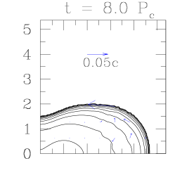
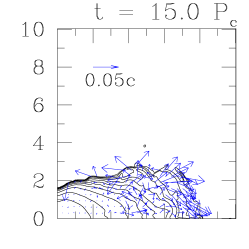
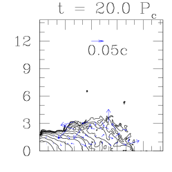
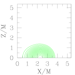
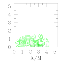
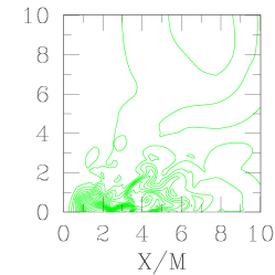
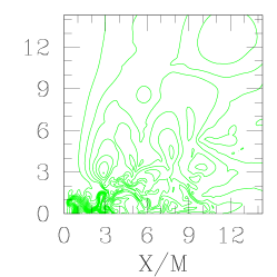
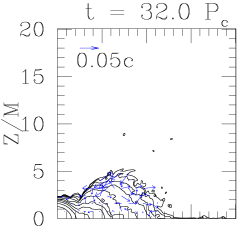
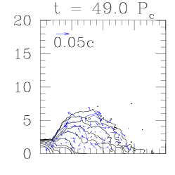
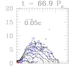
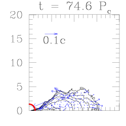
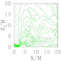
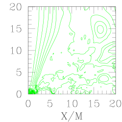
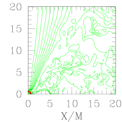
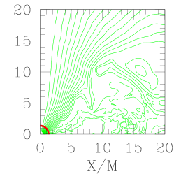
Figure 1: Snapshots of rest-mass density contours and poloidal magnetic field lines for star A at selected times. The first and third rows show snapshots of the rest-mass density contours and velocity vectors on the meridional plane. The second and fourth rows show the corresponding field lines (lines of constant $A_{\varphi}$) for the poloidal magnetic field at the same times. The density contours are drawn for $\rho_{0}/\rho_{\rm max}(0)=10^{-0.36i-0.09}~{}(i=0$–10), where $\rho_{\rm max}(0)$ is the maximum rest-mass density at $t=0$. The field lines are drawn for $A_{\varphi}=A_{\varphi,\rm min}+(A_{\varphi,\rm max}-A_{\varphi,\rm min})i/20~{}(i=1$–19), where $A_{\varphi,\rm max}$ and $A_{\varphi,\rm min}$ are the maximum and minimum values of $A_{\varphi}$, respectively, at the given time. The thick solid (red) curves denote the apparent horizon. In the last panel, the field lines are terminated inside the black hole at the excision boundary.

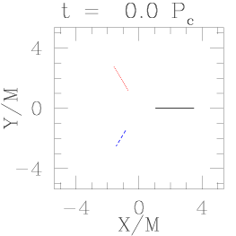
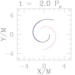
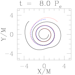
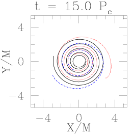
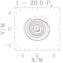
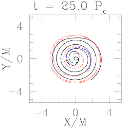
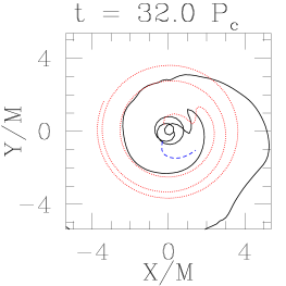
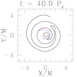
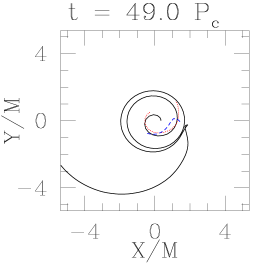
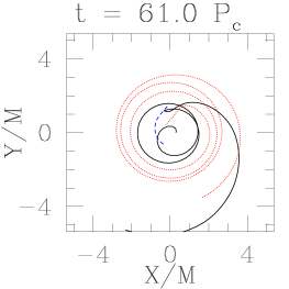
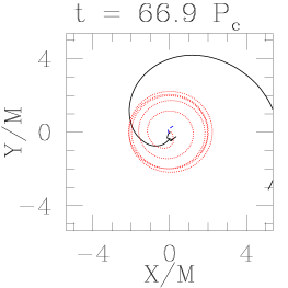
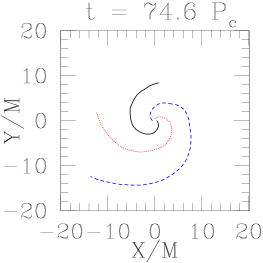
Figure 2: Snapshots of the projected 3D magnetic field lines for star A (see Appendix A for details) at selected times. Only three lines are drawn in each panel to prevent overcrowding of field lines.

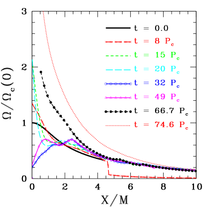
Figure 3: Angular velocity profiles for star A at selected times (corresponding to the times in Fig. 1). The last two profiles correspond to the moment of excision and a late time in the excision run.

Figure 1 shows the snapshots of density contours and poloidal magnetic field lines (lines of constant $A_{\varphi}$) in the meridional plane. Figure 2 shows the snapshots of three-dimensional (3D) magnetic field lines projected onto the equatorial plane.

In the early phase of the evolution, the frozen-in poloidal magnetic fields lines are wound up by the differentially rotating matter, creating a toroidal field which grows linearly in time (see Fig. 2 and Fig. 4d) with the growth rate predicted by Eq. (7). When the magnetic field becomes sufficiently strong, magnetic stresses act back on the fluid, causing a redistribution of angular momentum. The core of the star contracts while the outer layers expand. At $t\gtrsim 6P_{c}$, the effect of the MRI becomes evident, as shown in Figs. 4c and  5, where we see that the maximum value of $|B^{x}|$ ($\equiv|B^{\varpi}|$) suddenly increases, growing exponentially for a short period (about one $e$-folding). We find that the MRI first occurs in the outer layers of the star near the equatorial plane. This is consistent with the linear analysis, as Eq. (12) together with star A’s angular velocity profile gives a shorter $t_{\rm MRI}$ near the outer part of the star. The effect of the MRI can be seen in Fig. 1, where we see that the poloidal field lines are distorted. The growth of the central density slows down once $|B^{x}|_{\rm max}$ and $|B^{y}|_{\rm max}$ ($\equiv|\varpi B^{\varphi}|_{\rm max}=|B^{T}|_{\rm max}$) saturate at $t\sim 20P_{c}$. This may be caused by MRI-induced turbulence redistributing some of the angular momentum to slow down the contraction of the core. The amplitude of the toroidal field begins to decrease after $t\gtrsim 20P_{c}\sim t_{A}$ (see Figs. 2 and 4d) and the core of the star becomes less differentially rotating (Fig. 3). This is consistent with the results of Shapiro , which predict that the magnetic field growth by magnetic winding should saturate after an Alfvén time, the magnetic energy having grown to an appreciable fraction of the initial rotational kinetic energy.

The combined effects of magnetic braking and MRI eventually trigger gravitational collapse to a black hole at $t\approx 66P_{c}\approx 36(M/2.8M_{\odot})~{}{\rm ms}$ when an apparent horizon forms. A collimated magnetic field forms near the polar region at this time (see Fig. 1). However, a substantial amount of toroidal field is still present (see Fig. 2). Without black hole excision, the simulation becomes inaccurate soon after the formation of the apparent horizon because of grid stretching. To follow the subsequent evolution, a simple excision technique is employed alcubierre ; excision . We are able to track the evolution for another $300M\approx 8P_{c}$. We find that not all the matter promptly falls into the black hole. The system settles down to a quasiequilibrium state consisting of a black hole surrounded by a hot torus and a collimated magnetic field near the polar region (see the panels corresponding to time $t=74.6P_{c}$ in Fig. 1). The irreducible mass of the black hole is about $0.9M$ and the rest-mass of the torus is about $0.1M$ (Fig. 7). We estimate that $J/M^{2}\sim 0.8$ for the final black hole. This system is a promising central engine for the short-hard gamma-ray bursts (see Sec. VI.5 and GRB2 ).

VI.1.2 Resolution study

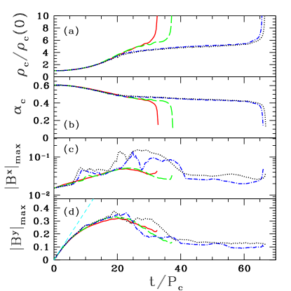
Figure 4: Evolution of the central rest-mass density $\rho_{c}$, central lapse $\alpha_{c}$, and maximum values of $|B^{x}|$ and $|B^{y}|$. $|B^{x}|_{\rm max}$ and $|B^{y}|_{\rm max}$ are plotted in units of $\sqrt{\rho_{\max}(0)}$. The solid (red), long-dashed (green), dot-dash (blue), and dotted (black) curves denote the results with $N$=250, 300, 400, and 500 respectively. The dashed (cyan) line in (d) represents the predicted linear growth of $|B^{y}|_{\rm max}$ at early times from Eq. (7).

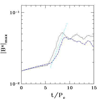
Figure 5: Evolution of $|B^{x}|_{\rm max}$ plotted in the same units as in Fig. 4 for the two highest resolution runs of star A. The dot-dashed (blue), and dotted (black) curves denote the results with $N$=400 and 500, respectively. The dashed (cyan) line represents an approximate slope $\omega=0.18/P_{c}$ for the exponential growth rate of the MRI, $\delta B^{x}\propto e^{\omega t}$.

Four simulations were performed with different resolutions (see Fig. 4): $N=$250, 300, 400 and 500. We find that the results converge approximately when $N\gtrsim 400$. On the other hand, results are far from convergent for $N\lesssim 300$. For example, $|B^{x}|_{\rm max}$ is much smaller at lower resolutions than for runs with higher resolutions, and the growth rate of $|B^{x}|_{\rm max}$ is underestimated. Hence, the effect of MRI, which is responsible for the growth of $|B^{x}|_{\rm max}$, is not computed accurately for low resolutions. This is because the wavelength of the fastest growing MRI mode is not well-resolved for low resolutions. We find that we need a resolution $\Delta/\lambda_{\rm max}\lesssim 0.14$ ($N\gtrsim 400$) in order to resolve the MRI modes. The straight dashed line in Fig. 4d corresponds to the linear growth rate predicted by Eq. (7). This slope agrees with the actual growth of $|B^{y}|_{\rm max}$ in the early (magnetic winding) phase of the simulation, but as back-reaction (magnetic braking) becomes important, the toroidal field begins to saturate.

Figure 5 shows the onset of the MRI in more detail for the two highest resolutions. Also shown is an approximate fit to the growth rate (the short dashed line). This line shows that the perturbation grows approximately as $\delta B^{x}\propto e^{\omega t}$, where $\omega\approx 0.18/P_{c}$. This is a somewhat lower rate than that predicted from linear theory, which gives $\omega_{\rm max}\sim 1/P_{c}$, where $\omega_{\rm max}$ corresponds to the fastest growing MRI mode. This discrepancy could be due to the fact that the linear analysis is inaccurate by a significant factor. One drawback of the linear analysis is the assumption of Newtonian gravity, but star A is highly relativistic. In addition, the linear analysis treats the MRI as a purely local phenomenon, assuming a uniform background state over length scales much longer than the wavelengths of the perturbations. However, since the expected $\lambda_{\rm max}$ is only one order of magnitude smaller than the initial equatorial radius, these assumptions may lead to significant discrepancies between the predicted and actual properties of the MRI.

VI.1.3 Evolution of the energies vs. time

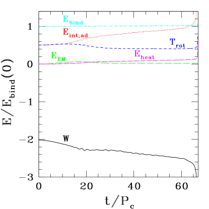
Figure 6: Components of the energy vs. time for star A. All energies are normalized to the binding energy at $t=0$, where the binding energy is defined as $E_{\rm bind}\equiv M_{0}-M$. In the evolution, $E_{\rm bind}$ should be nearly conserved.

Figure 6 shows the evolution of various energies defined in Sec. IV.4. We see that the magnetic energy $E_{\rm EM}$ remains small throughout the entire evolution, even though the magnetic field drives the secular evolution. The gravitational potential energy $W$ and the adiabatic part of the internal energy $E_{\rm int,ad}$ change the most, which results from the drastic change in the configuration of the star. The rotational kinetic energy decreases substantially before the core collapses, presumably because the bulk of the mass of the star rotates slower than at $t=0$. A substantial amount of heat ($E_{\rm heat}$) is also generated by shocks.

VI.1.4 Evolution with excision

Figure 7: Evolution of the irreducible mass and the total rest-mass outside the apparent horizon. (Here, $r_{\rm AH}$ is the local coordinate radius of the apparent horizon.)

Soon after the formation of the apparent horizon, the simulation becomes inaccurate due to grid stretching and an excision technique is required to follow the subsequent evolution. During the excision evolution, we track the irreducible mass of the black hole by computing the area of the apparent horizon $\mathcal{A}_{\rm AH}$ and using $M_{\rm irr}\approx\sqrt{\mathcal{A}_{\rm AH}/16\pi}$. The irreducible mass and the total rest mass outside the apparent horizon are shown in Fig. 7. The total ADM mass of the final state system, consisting of a BH surrounded by a massive accretion torus, is well defined. In contrast, there is no rigorous definition for the mass of the black hole itself. To obtain a rough estimate, we proceed as follows. First, the angular momentum of the black hole is computed from

$$J_{\rm hole}=J-J_{\rm matter}(r>r_{AH})$$ (61)

where the angular momentum of the matter outside the horizon is given by

$$J_{\rm matter}(r>r_{AH})=\int_{V,r>r_{AH}}\tilde{S}_{\varphi}d^{3}x\ ,$$ (62)

as in Eq. (51). Then to estimate the black hole mass, we use

$$M_{\rm hole}\approx\sqrt{M_{\rm irr}^{2}+(J_{\rm hole}/2M_{\rm irr})^{2}}\ ,$$ (63)

which is an approximate relation for the spacetime of our numerical simulation, but would be exact for a Kerr spacetime. We thus find $M_{\rm hole}\sim 0.9M$, where $M$ is the total ADM mass of the system, and $J_{\rm hole}/M_{\rm hole}^{2}\sim 0.8$.

The black hole grows at an initially rapid rate following its formation. However, the accretion rate $\dot{M}_{0}$ gradually decreases and the black hole settles down to a quasi-equilibrium state. By the end of the simulation, $\dot{M}_{0}$ has decreased to a steady rate of $\approx 0.01M_{0}/P_{c}$, giving an accretion timescale of $\sim 10$–$20P_{c}\approx 5$–$10~{}{\rm ms}(M/2.8M_{\odot})$. Also, we find that the specific internal thermal energy in the torus near the surface is substantial because of shock heating. The possibility that this sort of system could give rise to a GRB is discussed in Section VI.5 and GRB2 .

VI.1.5 Constraint violations

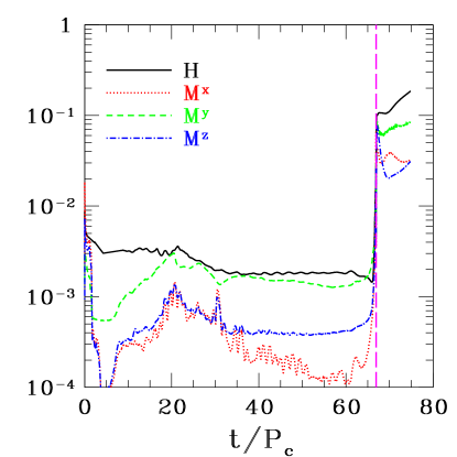
Figure 8: L2 norms of the errors in the Hamiltonian ($\mathcal{H}$) and momentum constraints ($\mathcal{M}^{i}$) for star A. The long-dashed, vertical (magenta) line represents the initial time for the excision run.

We monitor the violation of Hamiltonian and momentum constraints during the evolution. Figure 8 shows the L2 norm of the constraints. We see that in the pre-excision phase, the violation of all constraints are a few $\times 10^{-3}$. Prior to excision, the constraints are satisfied to better than 1%. This indicates that our numerical evolution data accurately satisfy the constraint equations. After excision, the constraint errors jump to $\sim 10$%, but they remain constant for $\gtrsim 300M\approx 8P_{c}$. We thus can track the evolution reliably for $\gtrsim 2800M$ in total, which is a nontrivial feat for highly relativistic, nonvacuum, and dynamical spacetime simulations.

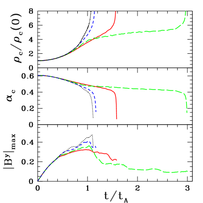
Figure 9: Selected parameters plotted against scaled time ($t/t_{\rm A}$) for evolutions of star A with four different magnetic field strengths: $C=1.25\times 10^{-3}$ (solid red lines), $C=2.5\times 10^{-3}$ (green long-dashed lines), $C=5.0\times 10^{-3}$ (blue short-dashed lines), and $C=10^{-2}$ (black dotted lines). All runs were performed with the same resolution ($400^{2}$ zones with outer boundaries at $20M$). When plotted against scaled time, the curves line up at early times ($t\mathrel{\raise 1.29167pt\hbox{$<$}\mkern-14.0mu\lower 2.58334pt\hbox{$\sim$}}0.5t_{\rm A}=11P_{c}$) when the evolution is dominated by magnetic winding.

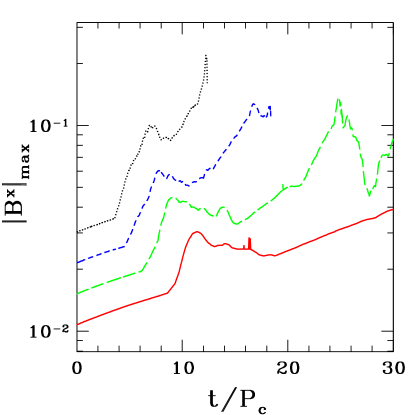
Figure 10: Maximum value of $|B^{x}|$ plotted vs. $t/P_{c}$ for evolutions of star A with four different magnetic field strengths. The line styles correspond to the same values of $C$ as in Fig. 9. The behavior of $|B^{x}|_{\rm max}$ is dominated by the effects of the MRI and thus does not scale with the Alfvén time. The curves corresponding to the two highest values of $C$ (dotted and dashed) terminate at the time when the star collapses.

VI.2 Star A, comparison of different values of $C$

In order to test the scaling of our results for different values of the initial magnetic field strength, we have examined three other values of $C$ in addition to the value of $2.5\times 10^{-3}$ chosen for the results of Section VI.1. Namely, we consider $C=\left\{1.25,2.5,5.0,10\right\}\times 10^{-3}$, and the results are shown in Figs. 9 and 10. For the portion of the simulations in which magnetic winding dominates, the behavior is expected to scale with the Alfvén time Shapiro . In other words, the same profiles should be seen for the same value of $t/t_{A}$. (The Alvén time is inversely proportional to the magnetic field strength and hence proportional to $C^{-1/2}$.) From Fig. 9, it is evident that this scaling holds very well for the toroidal field and for the central density and lapse, while $t\mathrel{\raise 1.29167pt\hbox{$<$}\mkern-14.0mu\lower 2.58334pt\hbox{$\sim$}}0.4t_{A}$. After the toroidal field saturates, the evolution is driven mainly by the MRI, which does not scale with the Alfvén time. The scaling also does not hold during the collapse phase, when the evolution is no longer quasi-stationary. Though the scaling breaks down at late times in these simulations, the qualitative outcome is the same in all cases.

The behavior of $|B^{x}|_{\rm max}$ for these four different values of $C$ is shown in Fig. 10. The sudden sharp rise of $|B^{x}|_{\rm max}$ signals the onset of the MRI, and the approximate agreement of the slopes for different values of $C$ indicates that the exponential growth rate of the MRI does not depend on the initial magnetic field strength (as expected from the linear analysis). In cases with a very weak initial magnetic field, turbulence induced by the MRI may become important much earlier than the effects of magnetic braking, since the timescale for the growth of the MRI does not depend on the initial magnetic field strength. In this case, the scaling with $t_{A}$ would not hold during any phase of the evolution. However, since both the MRI and magnetic braking lead to similar angular momentum transfer, the qualitative outcome may again be the same.

VI.3 Star B1

Here, we present results for the evolution of star B1 with $C=2.5\times 10^{-3}$. This run was performed with resolution $400^{2}$ and outer boundaries located at $4.5R$ ($36.4M$). Since this model is not hypermassive, the redistribution of angular momentum through MHD effects will not lead to collapse. However, since this star is ultraspinning and angular momentum is conserved in axisymmetric spacetimes, it cannot relax to a uniform rotation state everywhere unless a significant amount of angular momentum can be dumped to the magnetic field. We find that this model simply seeks out a magnetized equilibrium state which consists of a fairly uniformly rotating core surrounded by a differentially rotating torus. This is similar to the final state we found in DLSS for the same model when evolved with shear viscosity.

Figure 11: Evolution of central rest-mass density $\rho_{c}$, central lapse $\alpha_{c}$, maximum values of $|B^{x}|$ and $|B^{y}|$ for star B1. The magnetic fields $|B^{x}|_{\rm max}$ and $|B^{y}|_{\rm max}$ are plotted in units of $\sqrt{\rho_{\rm max}(0)}$. Note that the lines become fairly horizontal at late times, indicating that an equilibrium has been reached. The dashed line in (c) represents an approximate slope of $\omega=(0.37/P_{c})$ for the exponential growth rate of the MRI, $\delta B^{x}\propto e^{\omega t}$. The dashed line in (d) represents the predicted linear growth of $|B^{y}|_{\rm max}$ computed from Eq. (7).

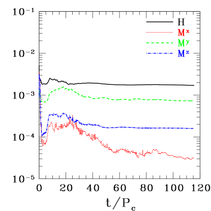
Figure 12: L2 norms of the errors in Hamiltonian and momentum constraints during the evolution of star B1.

Figure 11 presents the evolution of some relevant quantities for this case. From the central density and lapse, it is evident that the star has settled into a more compact equilibrium configuration. This is consistent with the expectation that magnetic braking should transfer angular momentum from the core to the outer layers. A brief episode of poloidal magnetic field growth due to the MRI is indicated by the plot of $|B^{x}|_{\rm max}$ in Figure 11. The instability saturates and quickly dies away fn3 , leaving the strength of the poloidal field largely unchanged. Early in the evolution, the maximum value of the toroidal component $|B^{y}|$ rises due to magnetic winding. This growth saturates at $t\sim 10P_{c}\sim 0.5t_{A}$ . We note, however, that the toroidal magnetic field is non-zero in the final equilibrium state, though it is no longer growing due to magnetic winding. The accuracy of the spacetime evolution is demonstrated by Fig. 12, which shows that the Hamiltonian and momentum constraint errors remain very small throughout the simulation.

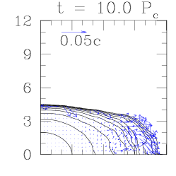
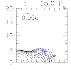
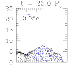
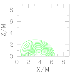
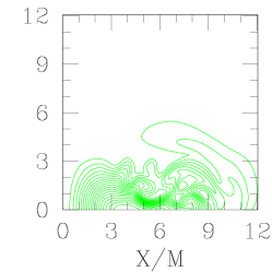
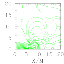
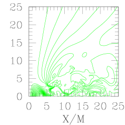
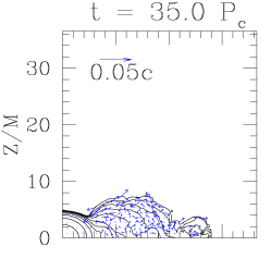
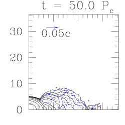
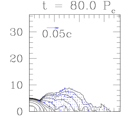
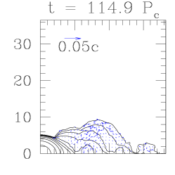
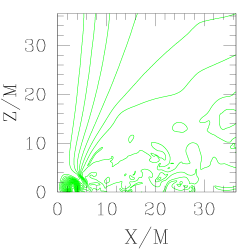
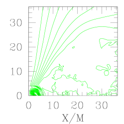
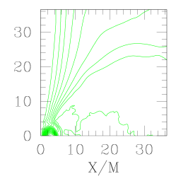
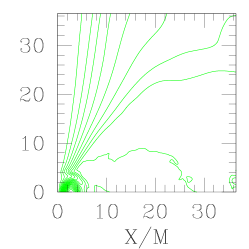
Figure 13: Snapshots of density contours and poloidal magnetic field lines for star B1. The first and third rows show snapshots of the rest-mass density contours and velocity vectors on the meridional plane. The second and fourth rows show the field lines (lines of constant $A_{\varphi}$) for the poloidal magnetic field at the same times as the first and third rows. The density contours are drawn for $\rho_{0}/\rho_{\rm max}(0)=10^{-0.36i-0.09}~{}(i=0$–10). The field lines are drawn for $A_{\varphi}=A_{\varphi,\rm min}+(A_{\varphi,\rm max}-A_{\varphi,\rm min})i/20~{}(i=1$–19), where $A_{\varphi,\rm max}$ and $A_{\varphi,\rm min}$ are the maximum and minimum values of $A_{\varphi}$ respectively at the given time. Note that the field lines and the density contours show little change for $t\gtrsim 35P_{c}$, indicating that the star has settled down to an equilibrium state.

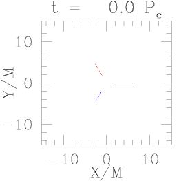
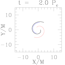
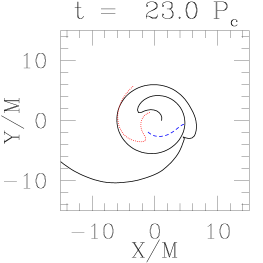
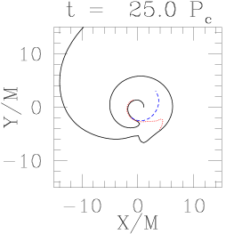
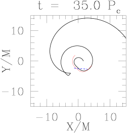
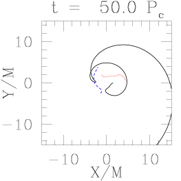
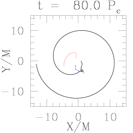
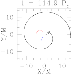
Figure 14: Snapshots of the projected 3D magnetic field lines for star B1.

Snapshots of the evolution in the $x$-$z$ plane are shown in Fig. 13. The density contours for times $t=0$ through $25.0P_{c}$ show that angular momentum redistribution leads to the formation of a more compact star surrounded by a torus. At $t=10P_{c}$, the distortions of the magnetic field lines due to the MRI are clearly visible. As the disk expands, magnetic field lines attached to this low density material open outward, eventually leading to the field structure seen in the last four times shown in Fig. 13, for which some field lines are still confined inside the star while others have become somewhat collimated along the $z$-axis. For $t\mathrel{\raise 1.29167pt\hbox{$>$}\mkern-14.0mu\lower 2.58334pt\hbox{$\sim$}}35P_{c}$, the density contours and poloidal magnetic field lines change very little, indicating that the system has reached an equilibrium state which is quite different from the initial state. The effects of magnetic braking in this case are demonstrated by the series of snapshots in Fig. 14, which is analogous to Fig. 2. The field lines become very tightly wound for $t\sim 10P_{c}$ and relax at later times. However, a significant toroidal field persists at late times when the system has essentially settled down to a final state.

Figure 15: Evolution of the degree of differential rotation $\Delta\Omega$ for star B1. At late times, $\Delta\Omega$ approaches a non-zero constant value. This shows that the final equilibrium state of star B1 is still differentially rotating.

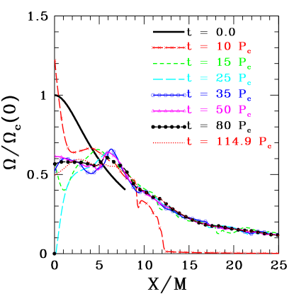
Figure 16: Angular velocity profiles at selected times (corresponding to the times in Fig. 13) for star B1.

Figure 17: Evolution of $\langle|B^{j}\partial_{j}\Omega|\rangle$ (normalized to unity at $t=0$). Note that this quantity drops toward zero at late time, indicating that the star is driven to a differentially rotating equilibrium state in which $\Omega$ is constant along the magnetic field lines.

In order to understand the behavior of this case, we plot in Fig. 15 the degree of differential rotation $\Delta\Omega$, defined as follows:

$$\Delta\Omega=\frac{\sqrt{\langle\Omega^{2}\rangle-\langle\Omega\rangle^{2}}}{\langle\Omega\rangle_{0}}\ ,$$ (64)

where the angular brackets refer to density weighted averages ($\langle f\rangle\equiv\int d^{3}x\rho_{*}f/M_{0}$) and $\langle\Omega\rangle_{0}$ is the average angular velocity at $t=0$. Rather than approaching zero at late times, this quantity approaches a roughly constant value. Thus, the equilibrium final state still has significant differential rotation. The evolution of the angular velocity profile for star B1 is shown in Fig. 16 for the equatorial plane. Figures. 13 and 16 suggest that the final state consists of a fairly uniformly rotating core surrounded by a differentially rotating torus. However, this differential rotation no longer winds up the magnetic field lines (i.e., the toroidal field strength does not grow). This is because the rotation profile has adjusted so that $\Omega$ is approximately constant along magnetic field lines. This is demonstrated in Fig. 17, which shows that

$$\langle|B^{j}\partial_{j}\Omega|\rangle\to 0$$ (65)

at late times. Since the rotation profile is adapted to the magnetic field structure, a stationary final state is reached which allows differential rotation and a nonzero toroidal field.

Since the final state is still differentially rotating and is threaded with magnetic fields, this configuration must be checked for the presence of the MRI. From the linear (and local) analysis discussed in Section II, we found that the predicted wavelength for the fastest growing mode is $\sim 2-3M$ at late times, whereas the radius of the final star is $\sim 6M$. (Since the local analysis does not take into account gradients in the vertical direction, it is qualitative at best in this regime. However, this does suggest that $\lambda_{\rm max}\sim R$.) Thus, the magnetic field is no longer weak, and the MRI is likely suppressed. This is corroborated by the fact that we do not see any rapid magnetic field growth at late times.

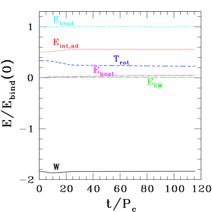
Figure 18: Components of the energy vs. time for star B1. All energies are normalized to the binding energy at $t=0$. In the evolution, $E_{\rm bind}$ should be nearly conserved.

Figure 19: Evolution of magnetic energy $E_{\rm EM}$ for star B1. The energy is normalized by the initial rotational kinetic energy of the star, $T_{\rm rot}(0)$.

Figure 18 shows the evolution of various energies. As in the case of star A, the magnetic energy $E_{\rm EM}$ shows a much smaller change in amplitude than $T_{\rm rot}$, $E_{\rm int,ad}$ and $W$. These results are very different from those found in Shapiro ; zys06 and from those of the star B2 evolution (see the next subsection), where the change in $E_{\rm EM}$ is comparable to the change in $T_{\rm rot}$. This is probably because star B1 is ultraspinning, in contrast to the “normal” models in Shapiro ; zys06 and star B2. Here the seed magnetic field in star B1 causes a substantial change (on a secular Alfvén timescale) in the structure of the star. The energies $E_{\rm int,ad}$, $T_{\rm rot}$ and $W$ readjust to the values of the new configuration, which is significantly different from the initial state. On the other hand, star B2 and the models studied in Shapiro ; zys06 show little or no change in the density profile. As a result, a decrease in $T_{\rm rot}$ results in an increase in $E_{\rm EM}$.

Figure 19 shows the evolution of the magnetic energy $E_{\rm EM}$, normalized to the initial rotational kinetic energy of the star, $T_{\rm rot}(0)$. The value of $E_{\rm EM}/T_{\rm rot}(0)$ rises from its initial value of $6.7\times 10^{-4}$ to a peak of $\sim 0.06$ (the corresponding field strength is about 90 times the initial field strength) mainly due to magnetic braking. Then it gradually decreases to the equilibrium value of 0.014. The final magnetic field strength $|B_{\rm final}|$ is about 4.5 times the initial value. In cgs units, we find that for the initial field considered here,

$$|B_{\rm final}|\sim 10^{17}\left(\frac{2M_{\odot}}{M}\right)~{}{\rm G}\ .$$ (66)

This field is comparable to the field strength of a magnetar. Since the strength of the initial seed magnetic field is much smaller than the strength when it saturates, it is possible that the final equilibrium state will be the same even if the initial seed field is much smaller than the present value. If this is true, a new-born neutron star with mass and angular momentum distribution similar to star B1 is likely to end up as a magnetar due to MHD processes.

VI.4 Star B2

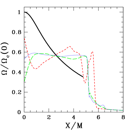
Figure 20: Angular velocity profiles in the equatorial plane for star B2 at times $t=0$ [thick solid (black) line], $t=8.1P_{c}\approx 1t_{A}$ [dashed (red) line], $t=32.5P_{c}\approx 4t_{A}$ [long dashed (green) line], and $t=46.5P_{c}\approx 5.8t_{A}$ [dotted (blue) line]. At late time ($t\gtrsim 30P_{c}\approx 4t_{A}$), the bulk of the star is nearly uniformly rotating.

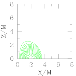
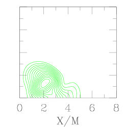
Figure 21: Snapshots of the rest-mass density contours and poloidal magnetic field lines for star B2 at times $t=0$ and $t=46.5P_{c}$. The first row shows snapshots of the rest-mass density contours on the meridional plane. The second row shows the corresponding field lines for the poloidal magnetic field at the same times. The density contours are drawn for $\rho_{0}/\rho_{\rm max}(0)=10^{-0.36i-0.09}~{}(i=0$–10), where $\rho_{\rm max}(0)$ is the maximum rest-mass density at $t=0$. The field lines are drawn for $A_{\varphi}=A_{\varphi,\rm min}+(A_{\varphi,\rm max}-A_{\varphi,\rm min})i/15~{}(i=1$–14), where $A_{\varphi,\rm max}$ and $A_{\varphi,\rm min}$ are the maximum and minimum values of $A_{\varphi}$, respectively, at the given time. The meridional components of the velocity (which are zero initially) at $t=46.5P_{c}$ are very small and so are not shown here.

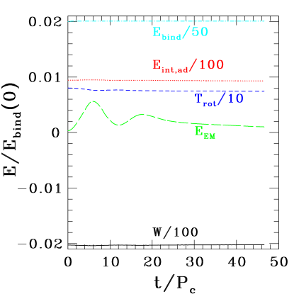
Figure 22: Components of the energy vs. time for star B2. All energies are normalized to the binding energy at $t=0$. Some quantities are normalized by an additional numerical factor (as indicated) to ease visualization.

Figure 23: Change of $T_{\rm rot}$ and $E_{\rm mag}$ vs. time. Here, $\delta T_{\rm rot}\equiv T_{\rm rot}-T_{\rm rot}(0)$ and $\delta E_{\rm mag}\equiv E_{\rm mag}-E_{\rm mag}(0)$.

Both stars B1 and B2 are nonhypermassive. However, star B1 is ultraspinning, whereas B2 is normal. We evolve this star with a seed magnetic field strength $C=2.5\times 10^{-3}$. Our simulation shows that this star evolves to a uniformly rotating configuration with little structural change (see Figs. 20 and 21).

Figure 21 shows the density contours and poloidal magnetic field at the initial time ($t=0$) and at $t=46.5P_{c}\approx 5.8t_{A}$. We see that the density profile of the star does not change appreciably. This is not surprising since the main effect of the MHD processes is to redistribute the angular momentum inside the star. However, the rotational kinetic energy of star B2 is not very large (the initial $T/|W|=0.040$). Hence, the change of the centrifugal force inside the star as a result of angular momentum transport does not disturb the initial equilibrium significantly, unlike the cases of stars A, B1 and C (see the next section).

Figure 22 shows the evolution of various energy components. Unlike stars A, B1 and C (see Fig. 28), the magnetic energy $E_{\rm EM}$ and rotational kinetic energy $T_{\rm rot}$ show the largest fractional variations. The adiabatic internal energy $E_{\rm int,ad}$ and gravitational potential energy $W$ have very small fractional changes. This is because the configuration of the star does not deviate significantly from the initial equilibrium (see Fig. 21). A large fraction of the growth of magnetic energy comes from the rotational kinetic energy (see Fig. 23). This is similar to the results reported in Shapiro ; zys06 .

VI.5 Star C

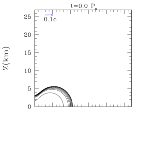
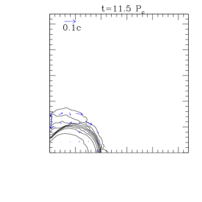
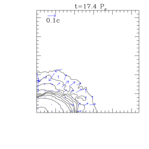
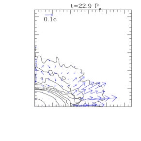
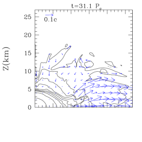
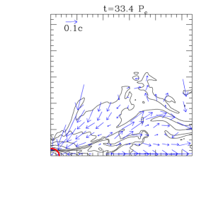
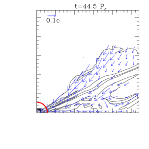
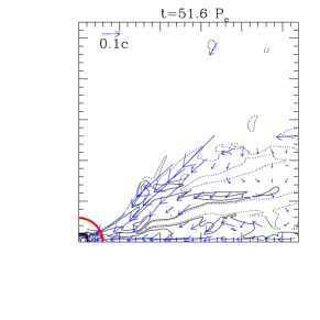
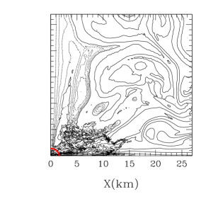
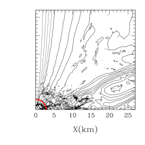
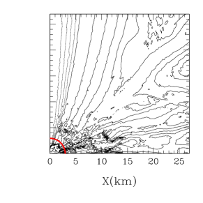
Figure 24: The same as Fig. 1 but for star C. The contours for the first and third rows are drawn for $\rho_{0}=10^{15-0.4i}~{}{\rm g/cm^{3}}~{}(i=0$–9). In the last two panels, curves with $\rho_{0}=10^{11}~{}{\rm g/cm^{3}}$ (solid curves) and with $\rho_{0}=5\times 10^{10}~{}{\rm g/cm^{3}}$ (dotted curves) are also drawn. The circular arc near the bottom-left corner in last three panels denotes an apparent horizon. The second and fourth rows show the poloidal magnetic field lines at the corresponding times. The solid contour curves are drawn for $A_{\varphi}=0.8(1-0.1i)A_{\varphi,{\rm max,0}}~{}(i=0$–9) and the dotted curves are for $A_{\varphi}=0.08(1-0.2i)A_{\varphi,{\rm max,0}}~{}(i=1$–4). Here, $A_{\varphi}=A_{\varphi,{\rm max,0}}$ is the maximum value of $A_{\varphi}$ at $t=0$. Note that the outer computational boundary in this simulation is located at $x\approx 54$ km and $z\approx 54$ km, and that $P_{c}\approx 0.2$ ms. The results with $N=601$ are shown here.

We next demonstrate that the same qualitative features of the MHD-induced hypermassive collapse discussed in Section VI.1 are also present with a more realistic EOS. To do this, we evolve star C, which was constructed using the hybrid EOS described in Section III. The ADM mass of this star is $2.65M_{\odot}$, which is 17% larger than the mass limit of a rigidly rotating neutron star for the adopted hybrid EOS. We choose an initial magnetic field with $C=7.1\times 10^{-3}$ as the fiducial model. In this case, the maximum strength of the magnetic field is $\sim 5\times 10^{16}$ G. The computational domain is $[0,L]$ in the $x$- and $z$-directions, with $L=5R_{\rm eq}\approx 54$km. We performed the same evolution with resolutions $N=501$, $601$, and $751$ to check convergence.

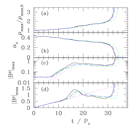
Figure 25: Evolution of the maximum rest-mass density $\rho_{\rm max}$, central lapse $\alpha_{c}$, and maximum values of $|B^{x}|$ and $|B^{y}|$ for star C. $|B^{x}|_{\rm max}$ and $|B^{y}|_{\rm max}$ are plotted in units of $\sqrt{\rho_{\max}(0)}$. The dashed (green), long-dashed (blue), and solid (black) curves denote the results with resolutions of $N=501$, $601$, and $751$ respectively. The dotted lines in (c) and (d) correspond to an exponential growth rate of $1/3P_{c}$ and predicted linear growth of $|B^{y}|_{\rm max}$ at early times from Eq. (7), respectively.

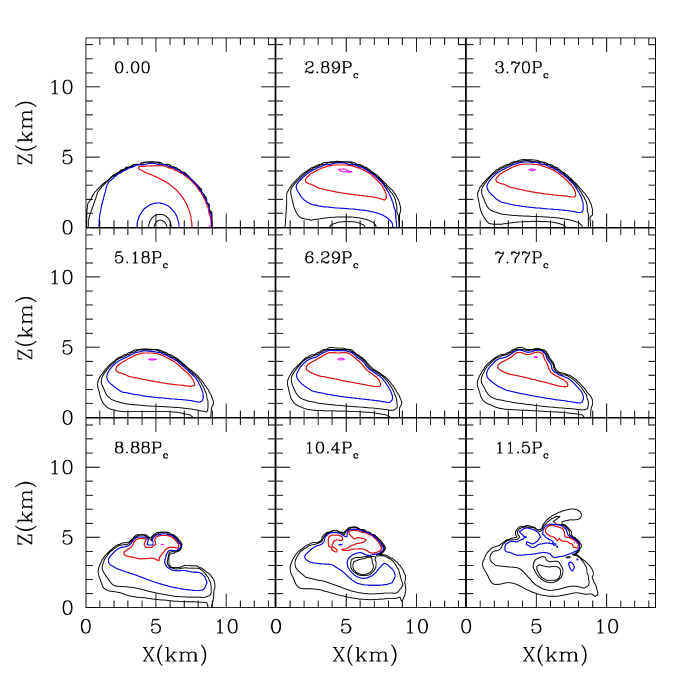
Figure 26: Contour curves for the ratio of the magnetic pressure $P_{\rm mag}$ to the gas pressure $P$ for $t\leq 11.5P_{c}$. The contour curves are drawn for $P_{\rm mag}/P=(P_{\rm mag}/P)_{\rm max}\times 10^{-0.01}$ (magenta), $10^{-0.5}$ (red), $10^{-1}$ (blue), and $10^{-0.5i}~{}(i=3,4)$ (black). The time $t$ is indicated for each snapshot.

Figure 27: Post-excision evolution of star C. The irreducible mass $M_{\rm irr}$ of the black hole and the rest mass of the torus surrounding the black hole settle down to their quasiequilibrium values at late times. The results with $N=601$ are shown.

Snapshots of the evolution at eight selected times are shown in Fig. 24. Figure 25 shows the evolution of the maximum density, central lapse, maximum values of $|B^{x}|$ and $|B^{y}|$ for the three values of $N$, indicating approximate convergence. The maximum values of $|B^{x}|$ and $|B^{y}|$ increase as the value of $N$ is increased. This is a natural consequence of the fact that the profile of the magnetic field is better resolved with increasing $N$.

As in the case of star A, the early phase of the evolution ($t\mathrel{\raise 1.29167pt\hbox{$<$}\mkern-14.0mu\lower 2.58334pt\hbox{$\sim$}}13P_{c}$) is dominated by magnetic winding. The linear growth then saturates and the subsequent evolution is dominated by the MRI (see the snapshots at $t=11.5P_{c}$ in Fig. 24 in which a clear distortion of the poloidal magnetic field lines is seen for $1~{}{\rm km}\mathrel{\raise 1.29167pt\hbox{$<$}\mkern-14.0mu\lower 2.58334pt\hbox{$\sim$}}x\mathrel{\raise 1.29167pt\hbox{$<$}\mkern-14.0mu\lower 2.58334pt\hbox{$\sim$}}4~{}{\rm km}$ and $z\mathrel{\raise 1.29167pt\hbox{$<$}\mkern-14.0mu\lower 2.58334pt\hbox{$\sim$}}3$ km). Soon after the onset of the MRI, the outer layers of the stellar envelope are blown off (see the snapshots for $t/P_{c}=11.5$–31.1). This explosion causes an expansion and redistribution of the magnetic field lines. Eventually, the removal of angular momentum from the central regions by the MRI results in collapse and black hole formation at $t\simeq 33P_{c}$.

The winding up of the toroidal magnetic field leads to strong, inhomogeneous magnetic pressure. The toroidal field is primarily generated in regions where the initial poloidal magnetic field has a significant radial component. Thus, material at high latitudes gains a high magnetic pressure at early times in the evolution. In Fig. 26, contour curves for the ratio of the magnetic pressure $P_{\rm mag}=b^{2}/2$ to the gas pressure $P$ are shown for $t\leq 11.5P_{c}$. It is seen that the region around $x\sim 5$ km and $z\sim 4$ km has the maximum ratio $P_{\rm mag}/P$, and the initial seed magnetic field is roughly radial in this region (see the first snapshots of Fig. 24). This region of strong magnetic pressure beneath the surface of the star is subject to the effects of magnetic buoyancy Kulsrud ; Parker , and toroidal magnetic field lines suddenly emerge from inside the HMNS, propelling material outward in the explosion (see the snapshots of Fig. 26 for $t/P_{c}\mathrel{\raise 1.29167pt\hbox{$>$}\mkern-14.0mu\lower 2.58334pt\hbox{$\sim$}}8$). This behavior may be due to the interchange instability Kulsrud . A similar magnetic buoyancy phenomenon is also observed in star A. However, unlike star C, the magnetic buoyancy does not cause an explosion in star A’s outer layers.

The time scale for the rearrangement of the field and the fluid due to buoyancy is approximately the same as that of the convection instability, and hence, of order $\tau_{\rm buoy}\sim(R^{2}H/GM)^{1/2}(\rho/\Delta\rho)^{1/2}$ or $\sim(R^{2}H/GM)^{1/2}(P/\Delta P_{\rm mag})^{1/2}$ Parker where $R$ and $H$ are the equatorial radius and scale height of the inhomogeneity of magnetic pressure and $\Delta\rho/\rho$ is the degree of inhomogeneity of the density due to the inhomogeneity of the magnetic pressure $\Delta P_{\rm mag}$. For the outer layers of star C, we find $H\sim 2$ km, and $\Delta P_{\rm mag}$ is approximately equal to the magnetic pressure $P_{\rm mag}$. Since $(P/P_{\rm mag})^{1/2}\sim c_{s}/V_{A}$, we have

$$\tau_{\rm buoy} \sim (R^{2}H/GM)^{1/2}c_{s}/V_{A}\sim t_{A}c_{s}/(GM/H)^{1/2}$$ (67)

$$\sim 0.4t_{A}\sim 0.9~{}{\rm ms}\ ,$$

which is comparable to the Alfv́en time scale. Indeed, this churning of field lines and fluid due to magnetic buoyancy seems to begin as soon as the toroidal field is wound up to a significant strength.

The formation of the black hole is accompanied by the formation of a torus (see the last three snapshots of Fig. 24). To follow the growth of the black hole due to accretion, the subsequent evolution of the system is computed with excision. Since the torus is magnetized, turbulent motion is induced which transports angular momentum outward in the accretion torus and encourages the accretion of matter onto the black hole.

In the accretion torus, the magnetic fields have a strong radial component (see, e.g., the snapshots at $t=44.5P_{c}$). This is because, during the formation of the black hole, some material in the envelope of the HMNS is ejected in the radial direction (see the snapshot at $t/P_{c}=31.1$), enhancing the radial magnetic field. The ejected matter soon falls onto the accretion torus, and compresses the magnetic fields. This process leads to a strong magnetic field in the accretion torus. (The typical value of $P_{\rm mag}/P$ is $10^{3}$–$10^{4}$ near the surface of the accretion torus.) As a result, material from high latitudes (which is originally blown away from the HMNS as a wind during the collapse) does not fall toward the equatorial plane, but collides with the surface of the torus, and then falls into the black hole along the surface of the torus (see the vector fields at $t=44.5P_{c}$). Hence, accretion occurs along high latitudes as well as along the equatorial plane. This scenario for black hole accretion is slightly different from those presented, e.g., in mg04 ; dvhkh05 . We also note that the last three panels of Fig. 24 show that the density of the accretion torus gradually decreases, indicating that accretion is quite rapid in the first $\sim 15P_{c}$ after the formation of the black hole.

For $t\mathrel{\raise 1.29167pt\hbox{$>$}\mkern-14.0mu\lower 2.58334pt\hbox{$\sim$}}45P_{c}$, the accretion relaxes to a steady rate $\dot{M}\sim 5\times 10^{-4}M_{0}/P_{c}\sim 5M_{\odot}/$s. The final state consists of a rotating black hole surrounded by a hot torus undergoing quasistationary accretion. At $t=50P_{c}$, the irreducible mass of the black hole is $M_{\rm irr}\approx 0.9M$, while the torus consists of $\sim 1\%$ of the original rest mass and $\sim 4\%$ of the original angular momentum of the system (see Fig. 27). During the simulation, $\sim 1\%$ of the total rest mass and $\sim 5\%$ of the total angular momentum escape from the computational domain through outflows. Following the same calculations as in Sec. VI.1.4, we estimate the mass and spin parameter of the black hole at $t\approx 50P_{c}$ to be $M_{\rm hole}\approx 0.98M$ and $J_{\rm hole}/M_{\rm hole}^{2}\approx 0.75$.

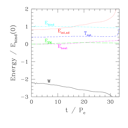
Figure 28: Components of the energy vs. time for star C. All energies are normalized to the binding energy at $t=0$, where the binding energy is defined as $E_{\rm bind}\equiv M_{0}-M$. In the evolution, $E_{\rm bind}$ should be nearly conserved.

Figure 28 shows the evolution of the various energies defined in Sec. IV.4. The magnetic energy $E_{\rm EM}$ reaches a value of at most 8% of the binding energy ($E_{\rm bind}$) throughout the entire evolution, even though the magnetic field drives the secular evolution. The gravitational potential energy $W$ and the adiabatic part of the internal energy $E_{\rm int,ad}$ change the most, which results from the drastic contraction of the stellar core. The fraction of $E_{\rm int,ad}$ is 60–70% larger than that for star A. This is simply due to the fact that star C is more compact. The rotational kinetic energy is nearly constant. A substantial amount of heat ($E_{\rm heat}$) is generated by shocks. When the apparent horizon first appears, this heat is $\sim 1\%$ of the rest-mass energy (i.e., $\sim 5\times 10^{52}$ ergs). Most of the heat is swallowed by the black hole, but a substantial fraction remains in the accretion torus (see below). Finally, the binding energy decreases by $\approx 7\%$ by the end of the pre-excision evolution. This is mainly due to the violation of approximate conservation of the ADM mass by $\approx 0.5\%$ and to the escape of $\sim 1\%$ of the mass from outer boundaries.

The internal energy in the torus corresponds to a typical thermal energy per nucleon of approximately $10^{2}$ MeV GRB2 , giving an equivalent temperature $T\approx$1–2 $\times 10^{11}$ K for the density $\sim 10^{10}$–$10^{12}~{}{\rm g/cm^{3}}$ if the assumed components are free nucleons, ultra-relativistic electrons, positrons, neutrinos, and thermal radiation MPN . The opacity to neutrinos inside the torus (considering only neutrino absorption and scattering interactions with nucleons) is MPN

$$\kappa\sim 7\times 10^{-17}\biggl{(}{T\over 10^{11}~{}{\rm K}}\biggr{)}^{2}~{}{\rm cm}^{2}~{}{\rm g}^{-1}.$$ (68)

Because of its high temperature and density, the torus is optically thick to neutrinos. Thus, the neutrino luminosity is estimated ST as $L_{\nu}\sim\pi R^{2}F$, where $R$ is the typical radius of the emission zone and $F$ is the flux from the neutrinosphere. In the diffusion limit, $F$ is approximated by

$$F\sim{7N_{\nu}\over 3}{\sigma T^{4}\over\kappa\Sigma}$$ (69)

where $\sigma$ is the Stefan-Boltzmann constant, $N_{\nu}$ is the number of thermal neutrino species, taken as 3, and $\Sigma$ is the surface density of the torus $\sim 10^{17}$–$10^{18}~{}{\rm g/cm^{2}}$. We then obtain

$$L_{\nu} \sim 2\times 10^{52}~{}{\rm ergs/s}\biggl{(}{R\over 10~{}{\rm km}}\biggr{)}^{2}$$ (70)

$$~{}~{}\times\biggl{(}{T\over 10^{11}~{}{\rm K}}\biggr{)}^{2}\biggl{(}{\Sigma\over 10^{17}~{}{\rm g/cm^{2}}}\biggr{)}^{-1}.$$

This luminosity will be present for the total duration of the accretion, $\sim 10$ ms. Since the torus has a geometrically thick structure, a substantial fraction of neutrinos are emitted toward the rotation axis, leading to enhanced neutrino-antineutrino pair annihilation along the axis. The pair annihilation could produce a relativistic fireball since the baryon density near the rotation axis is much lower than that in the torus. Furthermore, the luminosity is expected to have a strong time-variability because of the turbulent nature of the torus. Therefore, this massive and hot torus has many favorable properties which may explain a short GRB of energy $\sim 10^{48}$–$10^{49}$ ergs MPN . This possibility was explored by Shibata et al. in GRB2 .

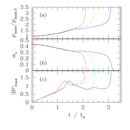
Figure 29: Evolution of the maximum rest-mass density $\rho_{\rm max}$, central lapse $\alpha_{c}$, and maximum values of $|B^{y}|/\sqrt{\rho_{\max}(0)}$ as a function of $t/t_{A}$ for star C with three values of $C$. The solid (blue), dashed (green), and long-dashed (red) curves correspond to results with $C=1.55\times 10^{-2}$, $7.1\times 10^{-3}$, and $3.8\times 10^{-3}$, respectively. The grid size is $N=601$ for all cases. The dotted line in (c) corresponds to the predicted linear growth of $|B^{y}|_{\rm max}$ at early times from Eq. (7).

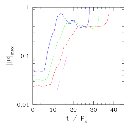
Figure 30: Evolution of the maximum values of $|B^{x}|/\sqrt{\rho_{\max}(0)}$ as a function of $t/P_{c}$ for star C with three values of $C$. The solid (blue), dashed (green), and long-dashed (red) curves denote the results with $C=1.55\times 10^{-2}$, $7.1\times 10^{-3}$, and $3.8\times 10^{-3}$, respectively. The grid size is $N=601$ for all cases. The dotted line segment corresponds to an exponential growth rate of $1/3P_{c}$.

Two other simulations are performed (with $N=601$) for different values of the initial magnetic field strength: $C=3.8\times 10^{-3}$ and $1.55\times 10^{-2}$. In Fig. 29, we show the evolution of the maximum density, central lapse, and maximum value of $|B^{y}|$ as a function of $t/t_{A}$. For star C, we find $t_{A}/P_{c}=8.94$, 13.4, and 17.9 for $C=1.55\times 10^{-2}$, $7.1\times 10^{-3}$, and $3.8\times 10^{-3}$, respectively. Figure 29 shows that the scaling relationship holds for $t/t_{A}\mathrel{\raise 1.29167pt\hbox{$<$}\mkern-14.0mu\lower 2.58334pt\hbox{$\sim$}}1$ as in Fig. 9. The scaling breaks down when $t/t_{A}\gtrsim 1$, indicating that the MRI and other effects such as magnetic buoyancy determine the evolution of the system.

In Fig. 30, we show the evolution of the maximum value of $|B^{x}|_{\rm max}$ as a function of $t/P_{c}$ for three values of $C$. As in Fig. 10, the sudden exponential growth signals the onset of the MRI, and the approximate agreement of the growth rate for different values of $C$ indicates that the exponential growth rate of the MRI does not depend on the initial magnetic field strength. After the exponential growth, the magnitude of $|B^{x}|_{\rm max}$ remains roughly constant until the dynamical collapse occurs. During this phase before collapse, the angular momentum is transported outward gradually by the turbulence. The duration for this angular momentum transport is $\sim 15P_{c}$ irrespective of the value of $C$ as long as $C\mathrel{\raise 1.29167pt\hbox{$>$}\mkern-14.0mu\lower 2.58334pt\hbox{$\sim$}}3.8\times 10^{-3}$. This indicates that the angular momentum is transported by a mechanism independent of the initial magnetic field strength (probably the turbulent transport associated with the MRI).

We note that the collapse time of the HMNS reported here depends slightly on the parameters of the atmosphere, although the timescales for growth of the magnetic field due to winding and the MRI do not. This is inevitable since, just before the collapse, the HMNS is only marginally stable against a quasiradial instability, and thus, a slight increase in the atmospheric mass-energy sensitively shortens the collapse time.

We have also studied models with masses slightly different from that of star C presented here. We find that the mass of the resulting torus varies significantly. For more massive stars, the torus mass is smaller. This is probably due to the fact that the star collapses sooner and hence there is less time for outward angular momentum transport. For a sufficiently large mass, the resulting torus mass is smaller than 0.1% of the total mass, which is probably too small for the system to trigger a short GRB. On the other hand, less massive stellar models result in larger torus masses. This result is interesting since it might explain the variety of short GRBs. The details of this study will be reported in a future paper.

VII Discussion and Conclusions

We have discussed in detail the evolution of magnetized HMNSs as first reported in DLSSS1 ; GRB2 . In addition, we have performed simulations of two differentially rotating, but nonhypermassive, neutron star models with the same initial magnetic field geometry. These simulations have revealed a rich variety of behavior with possible implications for astrophysically interesting systems such as binary neutron star remnants, nascent neutron stars, and GRBs, where magnetic fields and strong gravity both play important roles.

The two hypermassive models considered in this study, stars A and C, both collapse to BHs due to the influence of the initially poloidal, seed magnetic field. The early phase of evolution for both models is dominated by magnetic winding. As the strength of the toroidal magnetic field grows, the resulting magnetic stress begins to transport angular momentum from rapidly moving fluid elements in the inner region to the more slowly moving fluid elements in the outer layers. During this magnetic braking phase, the inner regions of the stars undergo quasistationary contraction, while the outer layers expand and begin to form a low-density torus.

The winding of the magnetic field proceeds until the back-reaction on the fluid becomes strong enough that the growth of the toroidal field ceases. This happens after roughly one Alfvén time. After several rotation periods, we also see the effects of the MRI. Plots of the poloidal magnetic field lines display perturbations with wavelengths similar to $\lambda_{\rm max}$ (the wavelength of the fastest growing mode estimated from the linear analysis). These perturbations first appear in the outer layers of the star, which is consistent with the linear analysis. In order to diagnose the sudden local growth of the poloidal magnetic field due to the MRI, we track the maximum value of $|B^{x}|$ on the grid. We found that $|B^{x}|_{\rm max}$ grows exponentially at a rate which does not depend on the strength of the initial magnetic field, in accord with the properties of the MRI. However, the growth rate observed in our numerical simulations differs significantly from that predicted by the linear analysis. This is due probably to the fact that (a) the linear analysis is based on Newtonian gravity, but the models we study here are highly relativistic, and/or (b) the small MRI wavelength assumption in the analysis might not be applicable to our magnetic field configuration.

The nonlinear outcome of the MRI is turbulence, and this turbulence leads to further angular momentum transport. Eventually, the inner cores of stars A and C become unstable and collapse to BHs. Surrounding the BHs, significant amounts of material remain in magnetized tori which have been heated considerably by shocks resulting from the turbulent motions of the fluid. This final state consisting of a BH surrounded by a massive, hot accretion disk may be capable of producing highly relativistic outflows and a fireball (either through $\nu-\bar{\nu}$ annihilation or MHD processes) and is hence a promising candidate for the central engine of short-hard GRBs. This model predicts that such GRBs should accompany a burst of gravitational radiation and neutrino emission from the HMNS delayed collapse.

The behavior of the nonhypermassive, ultraspinning star B1 under the influence of a seed magnetic field is quite different. Magnetic braking and the MRI operate in this model as well, leading to a mild contraction of the inner core and the expansion of the outer layers into a high angular momentum torus-like structure. The final state consists of a fairly uniformly rotating core surrounded by a differentially rotating torus. The remaining differential rotation does not shear the magnetic field lines (i.e. $\langle|B^{j}\partial_{j}\Omega|\rangle$ approaches zero in the final state), so that the toroidal field settles down. We find that this configuration is not subject to the MRI, probably because it is suppressed by the strong magnetic field (the MRI wavelength is comparable to the size of the star, and the standard local linear analysis breaks down in this regime). The rotation state of the final configuration naturally depends on the geometry of the initial magnetic field. On the other hand, the normal star B2 simply evolves to a uniformly rotating configuration.

Two issues in particular warrant further study. The first is the scaling behavior of our solutions. We begin our simulations with a seed magnetic field which, though far too weak to be dynamically important, may be significantly larger than magnetic fields present in HMNSs formed through stellar collapse or a binary neutron star merger. We have demonstrated that, by varying the strength of the initial magnetic field through a factor of $\sim 3$ (See Fig. 9), our evolution obeys the expected scaling during the magnetic winding phase, and the qualitative outcome of the simulations remains the same. However, since the MRI grows on a timescale $\sim\mbox{few}\times P_{c}$ regardless of the initial magnetic field strength, it is possible that, for very weak initial fields, the effects of the MRI could dominate the evolution long before the effects of magnetic braking become important. In this case, the scaling of our numerical results with the Alfvén time (relevant for magnetic winding) may break down. The relative importance of magnetic winding and the MRI for different seed field strengths deserves further study. Unfortunately, the wavelength of the fastest growing MRI mode becomes very difficult to resolve numerically as the strength of the initial magnetic field decreases. However, our results seem to indicate that magnetic braking and MRI-induced turbulence have similar effects in magnetized HMNSs. Thus, the qualitative features of the evolutions described here may also be present for HMNSs with much weaker initial seed fields.

Another issue which warrants further study concerns the effects on our evolutions of relaxing the axisymmetry assumption. Rapidly and differentially rotating neutron stars may be subject to bar and/or one-armed spiral mode instabilities which could affect the dynamics (though star A was shown in BSS ; DLSS to be stable against such instabilities, at least on dynamical timescales). Additionally, the development of the MRI in 2D differs from the 3D case hgb95 . Turbulence arises and persists more readily in 3D due to the lack of symmetry. More specifically, according to the axisymmetric anti-dynamo theorem moffatt78 , sustained growth of the magnetic field energy is not possible through axisymmetric turbulence. This phenomenon has been demonstrated by numerical simulations hb92 . However, McKinney and Gammie mg04 have performed axisymmetric simulations of magnetized tori accreting onto Kerr BHs and have found good quantitative agreement with the 3D results of De Villiers and Hawley dvhkh05 for the global quantities $\dot{E}/\dot{M}_{0}$ and $\dot{J}/\dot{M}_{0}$ fn4 , which are the rates of total energy and angular momentum falling into the horizon, normalized by the accretion rate. Though simulations in full 3D will eventually be necessary to capture the full behavior of magnetized HMNSs, the 2D results presented here likely provide (at least) a good qualitative picture.

Appendix A Drawing magnetic field lines

The vector potential $A^{i}$ is related to the magnetic field $B^{i}$ by $B^{i}=n_{\mu}\epsilon^{\mu ijk}\partial_{j}A_{k}$, where $\epsilon^{\alpha\beta\gamma\delta}$ is the Levi-Civita tensor. It is easy to show that in axisymmetry, the poloidal components of a magnetic field ($B^{\varpi}$ and $B^{z}$) are determined by $A_{\varphi}$ alone as follows:

$$\varpi\sqrt{\gamma}\,B^{\varpi} = -\partial_{z}A_{\varphi}\ ,$$ (71)

$$\varpi\sqrt{\gamma}\,B^{z} = \partial_{\varpi}A_{\varphi}\ .$$ (72)

Poloidal magnetic field lines are two-dimensional curves on which $d\varpi/dz=B^{\varpi}/B^{z}=-\partial_{z}A_{\varphi}/\partial_{\varpi}A_{\varphi}$. Hence we have

$$dA_{\varphi}=(\partial_{\varpi}A_{\varphi})d\varpi+(\partial_{z}A_{\varphi})dz=0$$ (73)

on the curves. This means that contours of constant $A_{\varphi}$ are the poloidal magnetic field lines. All the poloidal field lines shown in this paper are drawn by the contours of $A_{\varphi}$. There are two ways of calculating $A_{\varphi}$. One method is to integrate Eqs. (71) and (72). The other method is to evolve $A_{\varphi}$ according to the equation

$$\partial_{t}A_{\varphi}=\varpi\sqrt{\gamma}(v^{z}B^{\varpi}-v^{\varpi}B^{z})\ .$$ (74)

This equation can be derived from Eqs. (35) and (42) of bs03 .

In order to show the toroidal component of the magnetic field, we draw field lines projected onto the equatorial plane. To do this, we first choose three points $\varpi_{(j)}$ ($j=$1, 2, 3) in the equatorial plane so that at the given time,

$$A_{\varphi}(\varpi_{(j)},z_{\rm min})=A_{\varphi,{\rm min}}+(A_{\varphi,{\rm max}}-A_{\varphi,{\rm min}})j/4\ ,$$ (75)

where $A_{\varphi,{\rm max}}$ and $A_{\varphi,{\rm min}}$ are the maximum and minimum values of $A_{\varphi}$ at the given time fn5 , and $z_{\rm min}=0$ when there is no apparent horizon in the time slice. If there is an apparent horizon, we set $z_{\rm min}=0$ if $\varpi_{(j)}>0.5r_{AH}$ and $z_{\rm min}=\sqrt{0.25r_{AH}^{2}-\varpi_{(j)}^{2}}$ if $\varpi_{(j)}<0.5r_{AH}$. Here $r_{AH}$ is the coordinate radius of the apparent horizon. Next we integrate the equations

$$\frac{dx_{(j)}}{d\lambda} = B^{x}(x_{(j)},y_{(j)},z_{(j)})\ ,$$ (76)

$$\frac{dy_{(j)}}{d\lambda} = B^{y}(x_{(j)},y_{(j)},z_{(j)})\ ,$$ (77)

$$\frac{dz_{(j)}}{d\lambda} = B^{z}(x_{(j)},y_{(j)},z_{(j)})\ ,$$ (78)

with the initial locations $(x_{j},y_{j},z_{j})$ given by:

$$x_{(j)}|_{\lambda=0} = \varpi_{(j)}\cos\left[\frac{2(j-1)\pi}{3}\right],$$

$$y_{(j)}|_{\lambda=0} = \varpi_{(j)}\sin\left[\frac{2(j-1)\pi}{3}\right],$$

$$z_{(j)}|_{\lambda=0} = z_{\rm min}\ \ \ \ \ \ \ \ (j=1,2,3)\ .$$ (79)

Here $\lambda$ serves as a parameter of the 3D curves. The integration is terminated when the curve goes beyond the boundary of the grid. The projected field lines are the trajectories $(x_{(j)}(\lambda),y_{(j)}(\lambda))$ traced out by $\lambda$. On the other hand, the poloidal field lines determined by the contours of $A_{\varphi}$ are equivalent to the trajectories of $(\sqrt{x^{2}+y^{2}},z)$.

References

- (1) T. Zwerger and E. Müller, Astron. Astrophys. 320, 209, 1997.
- (2) M. Rampp, E. Müller, and M. Ruffert, Astron. Astrophys. 332, 969 (1998); H. Dimmelmeier, J. A. Font, and E. Müller, Astron. Astrophys. 388, 917 (2002); 393, 523 (2002); M. Shibata and Y. Sekiguchi, Phys. Rev. D 69, 084024 (2004); C. D. Ott, A. Burrows, E. Livne, and R. Walder, Astrophys. J. 600, 834 (2004).
- (3) Y. T. Liu and L. Lindblom, Mon. Not. R. Astron. Soc. 324, 1063 (2001); Y. T. Liu, Phys. Rev. D, 65, 124003 (2002).
- (4) F. A. Rasio and S. L. Shapiro, Astrophys. J. 432, 242 (1994); Class. Quant. Grav. 16 R1 (1999).
- (5) M. Shibata and K. Uryū, Phys. Rev. D 61, 064001 (2000).
- (6) J. A. Faber and F. A. Rasio, Phys. Rev. D 62, 064012 (2000).
- (7) T. W. Baumgarte, S. L. Shapiro, and M. Shibata, Astrophys. J. Lett. 528, L29 (2000).
- (8) I. A. Morrison, T. W. Baumgarte, S. L. Shapiro, and V. R. Pandharipande, Astrophys. J., 610, 941 (2004).
- (9) M. Shibata, K. Taniguchi, and K. Uryū, Phys. Rev. D 68, 084020 (2003).
- (10) M. Shibata, K. Taniguchi, and K. Uryū, Phys. Rev. D 71, 084021 (2005).
- (11) M. Shibata, and K. Taniguchi, submitted to Phys. Rev. D.
- (12) M. D. Duez, Y. T. Liu, S. L. Shapiro, and B. C. Stephens, Phys. Rev. D 69, 104030 (2004).
- (13) R. Narayan, B. Paczynski, and T. Piran, Astrophys. J. Lett. 395, L83 (1992); M. Ruffert and H.-T. Janka, Astron. Astrophys. 344, 573 (1999).
- (14) B. Zhang and P. Mészáros, Int. J. Mod. Phys. A 19, 2385 (2004); T. Piran, Rev. Mod. Phys. 76, 1143 (2005).
- (15) J. S. Bloom, et al., Astrophys. J., in press, astro-ph/0505480; E. Berger et al., Nature, in press, astro-ph/0508115; D. B. Fox, et al., Nature, 437, 845 (2005); J. Hjorth, et al., Nature, 437, 859 (2005).
- (16) M. D. Duez, Y. T. Liu, S. L. Shapiro, and B. C. Stephens, Phys. Rev. D 72, 024028 (2005).
- (17) M. Shibata and Y.-I. Sekiguchi, Phys. Rev. D 72, 044014 (2005).
- (18) L. Antón, O. Zanotti, J. A. Miralles, J. M. Martí, J. M. Ibáñez, J. A. Font, and J. A. Pons, Astrophys. J., in press, astro-ph/0506063 (2005).
- (19) M. D. Duez, Y. T. Liu, S. L. Shapiro, M. Shibata, and B. C. Stephens, Phys. Rev. Lett. 96, 031101 (2006) (astro-ph/0510653).
- (20) M. Shibata, M. D. Duez, Y. T. Liu, S. L. Shapiro, and B. C. Stephens, Phys. Rev. Lett. 96, 031102 (2006) (astro-ph/0511142).
- (21) S. L. Shapiro, Astrophys. J. 544, 397 (2000); J. N. Cook, S. L. Shapiro, and B. C. Stephens, Astrophys. J. 599, 1272 (2003); Y. T. Liu and S. L. Shapiro, Phys. Rev. D, 69, 104030 (2004).
- (22) L. Spitzer, Jr., Physical Processes in the Interstellar Medium (John Wiley, New York, 1978).
- (23) H. C. Spruit, Astron. and Astrophys., 349, 189 (1999)
- (24) V. P. Velikhov, Soc. Phys. JETP, 36, 995 (1959); S. Chandrasekhar, Proc. Natl. Acad. Sci. USA, 46, 253 (1960).
- (25) S. A. Balbus and J. F. Hawley, Astrophys. J. 376, 214 (1991)
- (26) S. A. Balbus and J. F. Hawley, Rev. Mod. Phys. 70, 1 (1998).
- (27) C. F. Gammie, Astrophys. J. 614, 309 (2004).
- (28) G. C. Cook, S. L. Shapiro, and S. A. Teukolsky, Astrophys. J. 422, 227 (1994).
- (29) A. Akmal, V. R. Pandharipande, and D. G. Ravenhall, Phys. Rev. C 58, 1804 (1998); F. Douchin and P. Haensel, Astron. Astrophys. 380, 151 (2001).
- (30) M. Shibata, T. W. Baumgarte, and S. L. Shapiro, Astrophys. J. 542, 453 (2000).
- (31) M. Shibata and T. Nakamura, Phys. Rev. D 52, 5428 (1995); T. W. Baumgarte and S. L. Shapiro, Phys. Rev. D 59, 024007 (1999).
- (32) H.-J. Yo, T. W. Baumgarte, and S. L. Shapiro, Phys. Rev. D 66, 084026 (2002);
- (33) M. D. Duez, S. L. Shapiro, and H.-J. Yo, Phys. Rev. D 69, 104016 (2004).
- (34) M. Alcubierre, B. Brügman, D. Pollney, E. Seidel, and R. Takahashi, Phys. Rev. D 69, 024012 (2004).
- (35) N. Ó Murchadha and J. W. York, Jr., Phys. Rev. D 10, 2345, (1974); J. W. York, Jr., in Sources of Gravitational Radiation, edited by L. L. Smarr (Cambridge Univ. Press, Cambridge, 1979); J. M. Bowen and J. W. York, Jr., Phys. Rev. D 21 2047 (1980).
- (36) R. M. Wald, General Relativity (Univ. of Chicago, Chicago, 1984), p. 297.
- (37) T. W. Baumgarte, G. B. Cook, M. A. Scheel, S. L. Shapiro, and S. A. Teukolsky, Phys. Rev. D 54, 4849 (1996); M. Shibata, Phys. Rev. D., 55, 2002 (1997).
- (38) M. D. Duez, P. Marronetti, S. L. Shapiro, and T. W. Baumgarte, Phys. Rev. D,67, 024004 (2003).
- (39) M. Alcubierre, S. Brandt, B. Brügmann, D. Holz, E. Seidel, R. Takahashi, and J. Thornburg, Int. J. Mod. Phys. D10, 273 (2001).
- (40) M. Alcubierre and B. Brügmann, Phys. Rev. D 63, 104006 (2001).
- (41) Note that this may be due to the artifact of the axisymmetry assumption. As explained in hb92 and MRIrev , this artifact is related to the axisymmetric anti-dynamo theorem moffatt78 .
- (42) Z. Etienne, Y. T. Liu, and S. L. Shapiro, in preparation.
- (43) See, e.g., Appendix I of S. L. Shapiro and S. A. Teukolsky, Black Holes, White Dwarfs, and Neutron Stars, Wiley Interscience (New York, 1983).
- (44) Di Matteo, R. Perna, and R. Narayan, Astrophys. J. 579, 706 (2002); W. H. Lee, E. R. Ruiz, and D. Page, Astrophys. J. 632, 421 (2005).
- (45) J. F. Hawley, C. F. Gammie, and S. A. Balbus, Astrophys. J. 440, 742 (1995); J. F. Hawley, Astrophys. J. 528, 462 (2000).
- (46) H. K. Moffatt, Magnetic Field Generation in Electrically Conducting Fluids (Cambridge Univ. Press, 1978).
- (47) J. F. Hawley and S. A. Balbus, Astrophys. J., 400, 595 (1992).
- (48) R. M. Kulsrud, Plasma Physics for Astrophysics (Princeton University Press, 2005), Sec. 7.3.1.
- (49) E. N. Parker, Cosmical Magnetic Fields (Oxford University Press, Newyork, 1979), Chap. 13.
- (50) J. C. McKinney and C. F. Gammie, Astrophys. J., 611, 977 (2004).
- (51) The expression for , and are as follows: , , and . All the integrands are evaulated at a constant spherical radius inside the black hole horizon.
- (52) J.-P. De Villiers, J. F. Hawley, J. H. Krolik, and S. Hirose, Astrophys. J. 620, 878 (2005).
- (53) T.W. Baumgarte and S.L. Shapiro, Astrophys. J. 585, 921 (2003).
- (54) Note that there may be more than one value of for each that satisfies Eq. (75). We choose the minimum value in this case. In the last panel in Fig. 2 (), Eq. (75) has no solution for all . We instead choose so that (=1, 2, 3).