On the formation of H$\alpha$ line emission around classical T Tauri stars

Abstract

We present radiative transfer models of the circumstellar environment of classical T Tauri stars, concentrating on the formation of the H$\alpha$ emission. The wide variety of line profiles seen in observations are indicative of both inflow and outflow, and we therefore employ a circumstellar structure that includes both magnetospheric accretion and a disc wind. We perform systematic investigations of the model parameters for the wind and the magnetosphere to search for possible geometrical and physical conditions which lead to the types of profiles seen in observations. We find that the hybrid models can reproduce the wide range of profile types seen in observations, and that the most common profile types observed occupy a large volume of parameter space. Conversely, the most infrequently observed profile morphologies require a very specific set of models parameters. We find our model profiles are consistent with the canonical value of the mass-loss rate to mass-accretion rate ratio ($\mu=0.1$) found in earlier magneto-hydrodynamic calculations and observations, but the models with $0.05<\mu<0.2$ are still in accord with observed H$\alpha$ profiles. We investigate the wind contribution to the line profile as a function of model parameters, and examine the reliability of H$\alpha$ as a mass accretion diagnostic. Finally, we examine the H$\alpha$ spectroscopic classification used by Reipurth et. al, and discuss the basic physical conditions that are required to reproduce the profiles in each classified type.

1 Introduction

T Tauri stars (TTS) are young ($\gtrsim 3\times 10^{6}\,\mathrm{yrs}$, Appenzeller & Mundt 1989) low-mass objects, and are the progenitors of solar-type stars. Classical T Tauri stars (CTTS) exhibit strong H$\alpha$ emission, and typically have spectral types of F–K. Some of the most active CTTS show emission in higher Balmer lines and metal lines (e.g., Ca ii H and K). They also exhibit excess continuum flux in the ultraviolet (UV) and infrared (IR). Their spectral energy distribution and polarisation data suggest the presence of circumstellar discs, which play an important role in regulating dynamics of gas flows around CTTS (e.g. Camenzind 1990).

Many observational studies (e.g., Herbig 1962; Edwards et al. 1994; Kenyon et al. 1994; Reipurth, Pedrosa & Lago 1996; Alencar & Basri 2000) of CTTS line profiles have revealed evidence for both outward wind flows and inward accretion flows, characterised by the blue-shifted absorption features in H$\alpha$ profiles and redshifted inverse P Cygni (IPC) profiles respectively. Typical mass-loss rates of CTTS are about $10^{-9}$ to $10^{-7}\,\mathrm{M_{\sun}\,yr^{-1}}$ (e.g., Kuhi 1964; Edwards et al. 1987; Hartigan, Edwards & Ghandour 1995), and the mass-accretion rates are also about $10^{-9}$ to $10^{-7}\,\mathrm{M_{\sun}\,yr^{-1}}$ (e.g., Kenyon & Hartmann 1987; Bertout, Basri & Bouvier 1988; Gullbring et al. 1998). Recent H$\alpha$ spectro-astrometric observations by Takami, Bailey & Chrysostomou (2003) provide indirect evidence for the presence of bipolar and monopolar outflows down to $\sim 1\,\mathrm{au}$ scale (e.g. CS Cha and RU Lup). Similarly, ESO VLT observations using high-resolution ($R=50\,000$) two-dimensional spectra of edge-on CTTS (HH 30, HK Tau B, and HV Tau C) by Appenzeller et al. (2005) show extended H$\alpha$ emission in the direction perpendicular to the obscuring circumstellar disc, suggesting the presence of the bipolar outflows. On an even larger scale, HST observations of HH30 (Burrows et al., 1996) trace the jet to within $\lesssim 30$ au of the star. The jet has a cone shape with an opening angle of $3^{\circ}$ between 70 and 700 au (Königl & Pudritz, 2000). Alencar & Basri (2000) found about 80 per cent of their sample (30 CTTS) show blue-shifted absorption components in at least one of the Balmer lines and Na D.

In the currently favoured model of accretion in CTTS, the accretion disc is disrupted by the magnetosphere, which channels the gas from the disc onto the stellar surface (e.g., Uchida & Shibata 1985; Königl 1991; Collier Cameron & Campbell 1993; Shu et al. 1994). This picture is supported by recent measurements of strong ($\sim 10^{3}\mathrm{G}$) magnetic fields in CTTS (e.g., Johns-Krull et al. 1999; Symington et al. 2005b) and by radiative transfer models which reproduce the gross characteristics of observed profiles for some CTTS (Muzerolle, Calvet & Hartmann 2001). In particular the magnetospheric accretion (MA) model explains blue-ward asymmetric emission line profiles as resulting from the partial occultation of the flow by the stellar photosphere and by the inner part of the accretion disc, while inverse P Cygni profiles in the MA model result from inflowing material at near free-fall velocities seen projected against hotspots on the stellar surface.

Despite these successes, the overwhelming observational evidence for outflows in CTTS suggests that the MA model is only one component of a complex circumstellar environment. Clearly, one must include the contribution of any wind/jet flow if one wishes to both accurately predict the mass-accretion rate and also determine the mass-loss rate of a CTTS via emission profile modelling. The first attempt in this direction was made by Alencar et al. (2005) who demonstrated that the observed H$\alpha$, H$\beta$ and Na D lines of RW Aur are better reproduced by the radiative transfer model which included a collimated disc-wind arising from near the inner edge of the accretion disc.

The main aim of this paper is to find a simple kinematic model which can reproduce the wide variety of the observed profiles, and to perform empirical studies of line formation in an attempt to place morphological classification schemes on a firmer physical footing. We will also discuss whether our model is consistent with some predictions made by recent (magneto-hydrodynamics) MHD studies i.e.  $\mu=\dot{M}_{\mathrm{wind}}/\dot{M}_{\mathrm{acc}}\approx 0.1$ (e.g. Königl & Pudritz 2000).

In Section 2, the model assumptions and the basic model configurations are presented. We discuss the radiative transfer model used to compute the profiles in Section 3, and the results of model calculations are given in Section 4. We discuss our results in the context of Reipurth’s classification scheme in Section 5, and our summary and conclusions are presented in Section 6.

2 Model configuration

In order to understand how the different parts of the CTTS circumstellar environment contribute to the formation of H$\alpha$, the model space is divided into four different regions: (1) a central continuum source, (2) the magnetospheric accretion flow, (3) the wind outflow, and (4) the accretion disc. Fig. 1 depicts the relative location of the regions in the model space. The density is assumed to be rotationally symmetric around the $z$-axis. The innermost radius of the magnetosphere at the equatorial plane coincides with the the inner radius of the accretion disc. From the innermost part of the accretion disc, the gas falls freely, moving along the magnetic field onto the surface of the star. In the following subsections we describe the details of the model components.

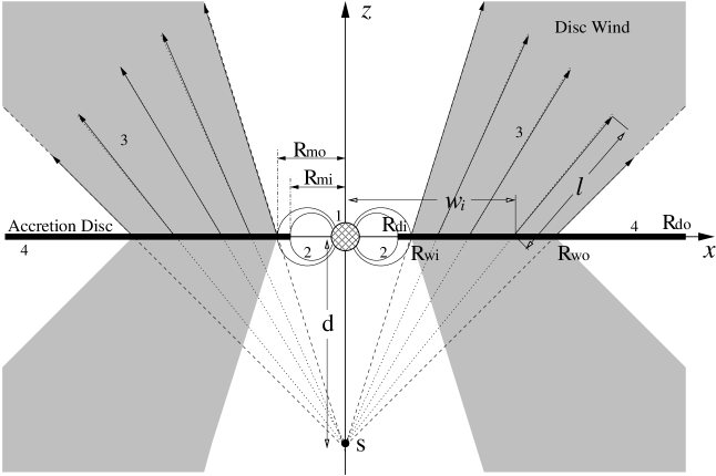
Figure 1: Basic model configuration of the disc-wind-magnetosphere hybrid model. The system consist of four components: (1) the continuum source located at the origin of the cartesian coordinates $\left(x,y,z\right)$ – the $y$-axis is into the paper, (2) the magnetospheric accretion flow, (3) the disc wind, and (4) the accretion disc. The disc wind originates from the disc surface between $w_{i}=R_{\mathrm{wi}}$ and $w_{i}=R_{\mathrm{wo}}$ where $w_{i}$ is the distance from the $z$ axis on the equatorial plane. The wind source points ($S$), from which the stream lines diverge, are placed at distance $d$ above and below the star. The degree of wind collimation is controlled by changing the value of $d$.

2.1 The continuum source

We adopt stellar parameters of a typical classical T Tauri star for the central continuum source, i.e. radius ($R_{*}$), mass ($M_{*}$), and effective temperature of the photosphere ($T_{\mathrm{ph}}$) are $2\,\mathrm{R_{\sun}}$, $0.5\,\mathrm{M_{\sun}}$, and $4000\,\mathrm{K}$ respectively. The model atmosphere of Kurucz (1979) with $T_{\mathrm{ph}}=4000\,\mathrm{K}$ and $\log g_{*}=3.5$ (cgs) defines the photospheric contribution to the continuum flux. The parameters are summarised in Table 1.

An additional continuum source is considered for models which include magnetospheric accretion: as the infalling gas approaches the stellar surface, it decelerates in a strong shock, and is heated to $\sim 10^{6}\,\mathrm{K}$. The X-ray radiation produced in the shock will be absorbed by the gas locally, and re-emitted as optical and UV light (Calvet & Gullbring 1998; Gullbring et al. 2000). This will create hot rings where the magnetic field intersects with the surface. We assume that the free-falling kinetic energy is thermalized in the radiating layer, and is re-emitted as blackbody radiation with a single temperature. With the parameters of the magnetosphere and the star given above (Table 1), about $8$ per cent of the surface is covered by the hot rings. In our model, the fraction of hot-ring coverage area is determined only by the geometry of the magnetosphere (Section 2.2). Gullbring et al. (2000) estimated the fractions of the hot-ring coverage area for three intermediate CTTS by using the observed UV and optical spectra. They found the range of fraction to be 0.3–3.0 per cent. This is smaller than the value adopted here; however, even if we use 1 per cent hot-ring area coverage model (by changing the width of the magnetosphere), we find the line shapes of H$\alpha$ do not change significantly (see also Fig. 5 of Muzerolle et al. 2001).

If the mass-accretion rate is $10^{-7}\,\mathrm{M_{\sun}\,yr^{-1}}$, the ratio of the accretion luminosity to the photospheric luminosity is about $0.5$, and the corresponding temperature of the hot rings is about $6400\,\mathrm{K}$. The luminosity ratio and the temperature depend on an adopted mass-accretion rate. The continuum emission from the hot rings is taken into account when computing the line profiles.

Table 1: Summary of the reference classical T Tauri star model parameters. Note that a typical mass-accretion rate of CTTS is $\sim 3\times 10^{-8}\,\mathrm{M_{\sun}\,yr^{-1}}$ (e.g. Gullbring et al. 1998; Calvet et al. 2004); however, a slightly higher mass-accretion rate is adopted here to demonstrate the effect of line-broadening more clearly (c.f. Section 4.1).

Parameters	$R_{*}$	$M_{*}$	$T_{\mathrm{ph}}$	$R_{\mathrm{mi}}$	$R_{\mathrm{mo}}$	$\dot{M}_{\mathrm{acc}}$	$\dot{M}_{\mathrm{wind}}$	$R_{\mathrm{di}}$	$R_{\mathrm{do}}$
	$\left[\mathrm{R_{\sun}}\right]$	$\left[\mathrm{M_{\sun}}\right]$	$\left[\mathrm{K}\right]$	$\left[R_{*}\right]$	$\left[R_{*}\right]$	$\left[\mathrm{M_{\sun}}\,\mathrm{yr^{-1}}\right]$	$\left[\mathrm{M_{\sun}}\,\mathrm{yr^{-1}}\right]$	$\left[R_{*}\right]$	$\left[\mathrm{au}\right]$
	$2.0$	$0.5$	$4000$	$2.2$	$3.0$	$10^{-7}$	$10^{-8}$	$2.2$	$100$

2.2 The magnetosphere

We adopt the MA flow model of Hartmann, Hewett & Calvet (1994), as done by Muzerolle et al. (2001) and by Symington, Harries & Kurosawa (2005a), in which the gas accretion on to the stellar surface from the innermost part of the accretion disc occurs through a dipolar stellar magnetic field. The magnetic field is assumed to be so strong that the gas flow does not affect the underlying magnetic field itself. As shown in Fig. 1 (region 2), the innermost radius ($R_{\mathrm{mi}}$) of the magnetosphere at the equatorial plane ($z=0$) is assigned to be the same as the inner radius ($R_{\mathrm{di}}$) of the accretion disc where the flow is truncated. In our models, $R_{\mathrm{mi}}$ and the outer radius ($R_{\mathrm{mo}}$) of the magnetosphere (at the equatorial plane) are set to be $2.2\,R_{*}$ and $3.0\,R_{*}$ respectively. The geometry of the magnetic field/stream lines is fixed for all calculations. We note that this magnetospheric geometry is identical to the “small/wide” model of Muzerolle et al. (2001).

The magnetic field and the gas stream lines are assumed to have the following simple form

$$r=R_{\mathrm{m}}\sin^{2}\theta$$ (1)

(see Ghosh, Pethick & Lamb, 1977) where $r$, and $\theta$ are the radial and the polar component of a field point position vector in the accretion stream. $R_{\mathrm{m}}$ is the radial distance to the field line at the equatorial plane ($\theta=\pi/2$), and its value is restricted between $R_{\mathrm{mi}}$ and $R_{\mathrm{mo}}$ (Fig. 1). Using the field geometry above and conservation of energy, the velocity and the density of the accreting gas along the stream line are found as in Hartmann et al. (1994).

The temperature structure of the magnetosphere used by Hartmann et al. (1994) is adopted here. They computed the temperature, assuming a volumetric heating rate which is proportional to $r^{-3}$, by solving the energy balance of the radiative cooling rate of Hartmann et al. (1982) and the heating rate (Hartmann et al., 1994). Martin (1996) presented a self-consistent determination of the thermal structure of the inflowing gas along the dipole magnetic field (equation 1) by solving the heat equation coupled to the rate equations for hydrogen. He found that main heat source is adiabatic compression due to the converging nature of the flow, and the major contributors to the cooling process are bremsstrahlung radiation and line emission from Ca II and Mg II ions. Muzerolle, Calvet, & Hartmann (1998) found that the line profile models computed according to the temperature structure of Martin (1996) do not agree with observations, unlike profiles based on the (less self-consistent) Hartmann et al. (1994) temperature distribution. It is clear that the temperature structure of the magnetosphere is still a large source of uncertainty in the accretion model; here we adopted the model of Hartmann et al. (1994).

2.3 The disc wind

The magneto-centrifugal wind paradigm, first proposed by Blandford & Payne (1982), has been often used to model the large-scale wind structure of T Tauri stars, or the observed optical jets (e.g. HH 30 jet by Burrows et al. 1996; Ray et al. 1996). The launching of the wind from a Keplerian disc is typically done by treating the equatorial plane of the disc as a mass-injecting boundary condition (e.g., Shu et al. 1994; Ustyugova et al. 1995; Ouyed & Pudritz 1997; Krasnopolsky et al. 2003). Depending on the location of the open magnetic fields anchored to the disc, two different types of winds are produced. If the field is constrained to be near the co-rotation radius of the stellar magnetosphere, an “X-wind” (Shu et al., 1994) is produced. If the open field lines are located in a wider area of the disc, a “disc-wind” similar to that of Königl & Pudritz (2000) is produced (see also Krasnopolsky et al. 2003). Recent reviews on the jet/wind-disc connection can be found in Königl & Pudritz (2000) and Pudritz & Banerjee (2005). Clearly there are several alternative outflow scenarios. Here we adopt a simple kinematical model, based on the disc-wind paradigm, which broadly represents the results of MHD simulations,

Knigge, Woods & Drew (1995) introduced the “split-monopole” kinematic disc-wind model in their studies of the UV resonance lines formed in the winds of cataclysmic variable stars. Their formalism provides a simple parameterisation of a disc wind that has similar properties to those found by MHD modelling. In this model, the outflow arises from the surface of the rotating accretion disc, and has a biconical geometry. The specific angular momentum is assumed to be conserved along a stream line, and the poloidal velocity component is assumed to be simply a radial from “sources” vertically displaced from the central star. Here we briefly describe the disc-wind model, and readers are referred to Knigge et al. (1995) and Long & Knigge (2002) for details.

The four basic parameters of the model are: (1) the mass-loss rate, (2) the degree of the wind collimation, (3) the velocity gradient, and (4) the wind temperature. The basic configuration of the disc-wind model is shown in Fig. 1. The disc wind originates from the disc surface, but the “source” point ($S$), from which the stream lines diverge, are placed at distance $d$ above and below the centre of the star. The angle of the mass-loss launching from the disc is controlled by changing the value of $d$. The mass-loss launching occurs between $R_{\mathrm{wi}}$ and $R_{\mathrm{wo}}$ where the former is set to be equal to the outer radius of the magnetosphere ($R_{\mathrm{mo}}$) and the latter is set to $1$ au, as in Krasnopolsky et al. (2003).

The local mass-loss rate per unit area ($\dot{m}$) is assumed to be proportional to the mid-plane temperature of the disc, and is a function of the cylindrical radius $w=\left(x^{2}+y^{2}\right)^{1/2}$, i.e.

$$\dot{m}\left(w\right)\propto\left[T\left(w\right)\right]^{4\alpha}\,\,.$$ (2)

The mid-plane temperature of the disc is assumed to be expressed as a power-law in $w$; thus, $T\propto w^{q}$. Using this in the relation above, one finds

$$\dot{m}\left(w\right)\propto w^{p}$$ (3)

where $p=4\alpha\times q$. The index of the mid-plane temperature power law is adopted from the dust radiative transfer model of Whitney et al. (2003) who found the innermost part of the accretion disc has $q=-1.15$. In order to be consistent with the collimated disc-wind model of Krasnopolsky et al. (2003) who used $p=-7/2$, the value of $\alpha$ is set to 0.76. The constant of proportionality in equation 3 is found by integrating $\dot{m}$ from $R_{\mathrm{wi}}$ to $R_{\mathrm{wo}}$, and normalising the value to the total mass-loss rate $\dot{M}_{\mathrm{wind}}$.

The azimuthal/rotational component of the wind velocity $v_{\phi}\left(w,z\right)$ is computed from the Keplerian rotational velocity at the emerging point of the stream line i.e. $v_{\phi}\left(w_{i},0\right)=\left(GM_{*}/w_{i}\right)^{1/2}$ where $w_{i}$ is the distance from the rotational axis ($z$) to the emerging point on the disc, and by assuming the conservation of the specific angular momentum along a stream line:

$$v_{\phi}\left(w,z\right)\,=v_{\phi}\left(w_{i},0\right)\,\left(\frac{w_{i}}{w}\right)\,\,.$$ (4)

Based on the canonical $\beta$ velocity law of hot stellar winds (c.f. Castor, Abbott & Klein 1975), the poloidal component of the wind velocity ($v_{p}$) parameterised as:

$$v_{p}\left(w_{i},l\right)=c_{\mathrm{s}}\left(w_{i}\right)+\left[f\,v_{\mathrm{esc}}-c_{\mathrm{s}}\left(w_{i}\right)\right]\left(1-\frac{R_{s}}{l+R_{s}}\right)^{\beta}$$ (5)

where $c_{\mathrm{s}}$, $f$, and $l$ are the sound speed at the wind launching point on the disc, the constant scale factor of the asymptotic terminal velocity to the local escape velocity (from the wind emerging point on the disc), and the distance from the disc surface along stream lines respectively. $R_{s}$ is the wind scale length, and its value is set to 10 $R_{\mathrm{wi}}$ by following Long & Knigge (2002).

Assuming mass-flux conservation and using the velocity field defined above, the disc wind density as a function of $w_{i}$ and $l$ can be written as

$$\rho\left(w_{i},l\right)=\frac{\dot{m}\left(w_{i}\right)}{v_{p}\left(w_{i},l\right)\,\left|\cos\delta\right|}\,\left\{\frac{d}{D\left(w_{i},l\right)\,\cos\delta}\right\}^{2}$$ (6)

where $D$ and $\delta$ are the distance from the source point ($S$) to a point along the stream line and the angle between the stream line and the disc normal, respectively. Fig. 2 shows the density and the velocity components along the mid stream line, passing through $w_{i}=\left(R_{\mathrm{wi}}+R_{\mathrm{wo}}\right)/2$, on the disc plane ($z=0$) for different values of the wind acceleration parameter $\beta$.

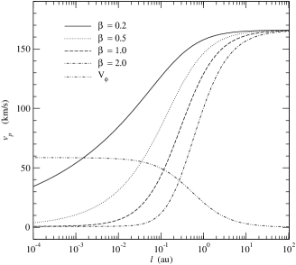
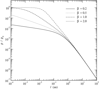
Figure 2: The dependency of the disc-wind density and velocity on the wind acceleration parameter $\beta$. The wind density $\rho$ (right panel) and the poloidal velocity component $v_{p}$ (left panel) along the stream line starting from the mid point of the wind launching zone, i.e. $\left(w,z\right)=\left(w_{\mathrm{mid}},0\right)$ where $w_{\mathrm{mid}}=\left(R_{\mathrm{wi}}+R_{\mathrm{wo}}\right)/2$, are shown as a function of the distance ($l$) from the wind launching point (c.f.  equations 5 and 6). The azimuthal velocity component ($v_{\phi}$), which is independent of $\beta$ (c.f. equation 4), is also shown in the left panel for comparison. The density is normalised to the density $\rho_{0}$ at the wind launching point for the $\beta=1.0$ case. The $v_{p}$ reaches the terminal velocity by 100 au for all $\beta$. In the far field ($l>10$ au), the density is approximately proportional to $\sim l^{-2}$.

2.4 The accretion disc

We adopt a simple analytical accretion disc model, the $\alpha$-disc ‘standard model’ (Shakura & Sunyaev 1973; Frank, King & Raine 2002) with the inner radius fixed at the inner radius of the magnetosphere at equatorial plane. This corresponds to Region 4 in Fig. 1.

2.4.1 Density and velocity

The disc density distribution is given by

$$\rho_{\mathrm{d}}\left(w,z\right)=\Sigma\left(w\right)\,\frac{1}{\sqrt{2\pi}h\left(w\right)}e^{-\left(\frac{z}{2h\left(w\right)}\right)^{2}}$$ (7)

where $w=\sqrt{x^{2}+y^{2}}$, $h$, $z$ and $\Sigma$ are the distance from the symmetry axis, the scale height, the distance from the disc plane, and the surface density at the mid-plane, respectively. The mid-plane surface density and the scale height are given as:

$$\Sigma\left(w\right)=\frac{5M_{\mathrm{d}}}{8\pi R_{\mathrm{do}}^{2}}\,w^{-3/4}$$ (8)

where $R_{\mathrm{do}}$ and $M_{\mathrm{d}}$ are the disc radius and the disc mass respectively, and

$$h\left(w\right)=0.05\,R_{\mathrm{do}}\,w^{9/8}\,.$$ (9)

With these parameters, the disc is slightly flared. The inner radius of the disc is set to $R_{\mathrm{di}}=R_{\mathrm{mi}}$ . The disc mass, $M_{\mathrm{d}}$, is assumed to be 1/100 of the stellar mass ($M_{*}$), and the outer disc radius ($R_{\mathrm{do}}$) is 100 au. The velocity of the gas/dust in the disc is assumed to be Keplerian.

Because of the geometrical constraints imposed by the magnetosphere and the disc wind, the finite height of the $\alpha$ disc causes an undesirable interface problem at the boundary; hence, the inner part ($R_{\mathrm{di}}<w<R_{\mathrm{wo}}$) of the disc is replaced by the geometrically thin (but opaque) disc. Since the emissivity of the disc at optical wavelengths is negligible, and the disc scale height is relatively small in the inner part of disc, this simplification is reasonable: the most important factor in determining the shape of the H$\alpha$ profiles is the finite height of the disc at large radii for large inclinations.

2.4.2 Dust model

In order to calculate the dust scattering and absorption cross section as a function of wavelength, the optical constants of Draine & Lee (1984) for amorphous carbon grains and Hanner (1988) for silicate grains are used. The model uses the “large grain” dust model of Wood et al. (2002) in which the dust grain size distribution is described by the following function:

$$n\left(a\right)da=\left(C_{\mathrm{C}}+C_{\mathrm{Si}}\right)\,a^{-p}\exp\left[-\left(\frac{a}{a_{c}}\right)^{q}\right]da$$ (10)

where $a$ is the grain size restricted between $a_{\mathrm{min}}$ and $a_{\mathrm{max}}$, and $C_{\mathrm{C}}$ and $C_{\mathrm{Si}}$ are the terms set by requiring the grains to completely deplete a solar abundance of carbon and silicon. The parameters adopted in our model are: $C_{\mathrm{C}}=1.32\times 10^{-17}$, $C_{\mathrm{Si}}=1.05\times 10^{-17}$, $p=3.0$, $q=0.6$, $a_{\mathrm{\mathrm{min}}}=0.1\,\mathrm{\mathrm{\mathrm{\mu m}}}$, $a_{\mathrm{\mathrm{max}}}=1000\,\mathrm{\mathrm{\mathrm{\mu m}}}$, and $a_{c}=50\,\mathrm{\mathrm{\mathrm{\mu m}}}$. This corresponds to Model 1 of the dust model used by Wood et al. (2002). See also their Fig. 3. The relative numbers of each grain is assumed to be that of solar abundance, C/H$\sim 3.5\times 10^{-4}$ (Anders & Grevesse, 1989) and Si/H$\sim 3.6\times 10^{-5}$ (Grevesse & Noels, 1993) which are similar to values found in the ISM model of Mathis, Rumpl & Nordsieck (1977) and Kim, Martin & Hendry (1994).

3 The radiative transfer model

We have extended the TORUS radiative transfer code (Harries 2000; Kurosawa et al. 2004; Symington et al. 2005a) to include the multiple circumstellar components described above. In previous calculations (Symington et al., 2005a), the model was used with a three-dimensional (3-D) adaptive mesh refinement (AMR) grid to investigate the line variability associated with rotational modulation of complex geometrical configurations of magnetospheric inflow (see also Kurosawa, Harries & Symington 2005). We modified the code to handle a two-dimensional (2-D) density distribution, and restricted our models to be axi-symmetric. Note that the velocity field is still in 3-D – the third component can be calculated by using symmetry for a given value of azimuthal angle.

The computation of H$\alpha$ is divided in two parts: (1) the source function calculation ($S_{\nu}$) and (2) the observed flux/profile calculation. In the first process, we have used the method of Klein & Castor (1978) (see also Rybicki & Hummer 1978; Hartmann et al. 1994) in which the Sobolev approximation method is applied. The population of the bound states of hydrogen are assumed to be in statistical equilibrium, and the gas to be in radiative equilibrium. Our hydrogen atom model consist of 14 bound states and a continuum. Readers are refer to Harries (2000) for details.

Monte Carlo radiative transfer (e.g. Hillier 1991), under the Sobolev approximation, can be used when (1) a large velocity gradient is present in the gas flow, and (2) the intrinsic line width is negligible compared to the Doppler broadening of the line. In our earlier models (Harries 2000; Symington et al. 2005a), this method was adopted since these conditions are satisfied. However, as noted and demonstrated by Muzerolle et al. (2001), even with a moderate mass-accretion rate ($\leavevmode\nobreak\ 10^{-7}\,\mathrm{M_{\sun}\,yr^{-1}}$), Stark broadening becomes important in the optically thick H$\alpha$ line. Muzerolle et al. (2001) also pointed out that the observed H$\alpha$ profiles from CTTS typically have the wings extending to $500\,\mathrm{km\,s^{-1}}$(e.g. Edwards et al. 1994; Reipurth et al. 1996) which cannot be explained by the infall velocity alone.

We have implemented the broadening mechanism following the formalism described by Muzerolle et al. (2001). First, the emission and absorption profiles are replaced from the Doppler to the Voigt profile, which is defined as:

$$H\left(a,y\right)\equiv\frac{a}{\pi}\int_{-\infty}^{\infty}\frac{e^{-y^{\prime 2}}}{\left(y-y^{\prime}\right)^{2}+a^{2}}\,dy^{\prime}$$ (11)

where $a=\Gamma/4\pi\Delta\nu_{\mathrm{D}}$, $y=\left(\nu-\nu_{0}\right)/\Delta\nu_{\mathrm{D}}$, and $y^{\prime}=\left(\nu^{\prime}-\nu_{0}\right)/\Delta\nu_{\mathrm{D}}$ (c.f. Mihalas 1978). $\nu_{0}$ is the line centre frequency, and $\Delta\nu_{\mathrm{D}}$ is the Doppler line width of hydrogen atom (due to its thermal motion) which is given by $\Delta\nu_{\mathrm{D}}=\left(2kT/m_{\mathrm{H}}\right)^{1/2}\times\left(\nu_{0}/c\right)$ where $m_{\mathrm{H}}$ is the mass of a hydrogen atom. The damping constant $\Gamma$, which depends on the physical condition of the gas, is parameterised by Vernazza, Avrett & Loeser (1973) as follows:

$$\Gamma = C_{\mathrm{rad}}+C_{\mathrm{vdW}}\left(\frac{n_{\mathrm{HI}}}{10^{16}\,\mathrm{cm^{-3}}}\right)\left(\frac{T}{5000\,\mathrm{K}}\right)^{0.3}$$ (12)

$$+\,C_{\mathrm{Stark}}\left(\frac{n_{e}}{10^{12}\,\mathrm{cm^{-3}}}\right)^{2/3}$$

where $n_{\mathrm{H\,I}}$ and $n_{e}$ are the number density of neutral hydrogen atoms and that of free electrons. Also, $C_{\mathrm{rad}}$, $C_{\mathrm{vdW}}$ and $C_{\mathrm{Stark}}$ are natural broadening, van der Waals broadening, and linear Stark broadening constants respectively. We adopt this parameterisation along with the values of broadening constants for H$\alpha$ from Luttermoser & Johnson (1992), i.e. $C_{\mathrm{rad}}=6.5\times 10^{-4}$ Å, $C_{\mathrm{vdW}}=4.4\times 10^{-4}$ Å  and $C_{\mathrm{Stark}}=1.17\times 10^{-3}$ Å. In terms of level populations and the Voigt profile, the line opacity for the transition $i\rightarrow j$ can be written as:

$$\chi_{l}=\frac{\pi^{1/2}e^{2}}{m_{e}c}f_{ij}n_{j}\left(1-\frac{g_{j}n_{i}}{g_{i}n_{j}}\right)H\left(a,y\right)$$ (13)

where $f_{ij}$, $n_{i}$, $n_{j}$, $g_{i}$and $g_{j}$ are the oscillator strength, the population of $i$-th level, the population of $j$-th level, the degeneracy of the $i$-th level, and the degeneracy of the $j$-th level respectively. $m_{e}$ and $e$ are the electron mass and charge (c.f. Mihalas 1978).

We further modified torus by replacing the Monte Carlo line transfer algorithm with a direct integration method (c.f. Mihalas 1978) for computing the observed flux as a function of frequency. The integration of the flux is performed in the cylindrical coordinate system $\left(p,\,q,\,t\right)$ which is obtained by rotating the original stellar coordinate system $\left(\rho,\,\phi,\,z\right)$ around the $y$ axis by the inclination of the line of sight. Note that the $t$-axis coincides with the line of sight with this rotation. The observed flux ($F_{\nu}$) is given by:

$$F_{\nu}=\frac{1}{4\pi d^{2}}\int_{0}^{p_{\mathrm{max}}}\int_{0}^{2\pi}p\,\sin q\,I_{\nu}\mathrm{\,d}q\,\mathrm{d}p$$ (14)

where $d$, $p_{\mathrm{max}}$, and $I_{\nu}$ are the distance to an observer, the maximum extent to the model space in the projected (rotated) plane, and the specific intensity ($I_{\nu}$) in the direction on observer at the outer boundary. For a given ray along $t$, the specific intensity is given by:

$$I_{\nu}=I_{0}e^{-\tau_{\infty}}+\int_{t_{0}}^{t_{\infty}}S_{\nu}\left(t\right)\,e^{-\tau}\mathrm{d}\tau$$ (15)

where $I_{0}$ and $S_{\nu}$ are the intensity at the boundary on the opposite to the observer and the source function ($\eta_{\nu}/\chi_{\nu}$) of the stellar atmosphere/wind at a frequency $\nu$. For a ray which intersects with the stellar core, $I_{0}$ is computed from the stellar atmosphere model of Kurucz (1979) as described in Section 2.1, and $I_{0}=0$ otherwise. If the the ray intersects with the hot ring on the stellar surface created by the accretion stream, we set $I_{0}=B_{\nu}\left(T_{\mathrm{ring}}\right)$ where $B_{\nu}$ is the Planck function and $T_{\mathrm{ring}}$ is the temperature of the hot ring. The initial position of each ray is assigned to be at the centre of the surface element ($\mathrm{d}A=p\,\sin q\,\mathrm{d}q\,\mathrm{d}p$). The code execution time is proportional to $n_{p}\,n_{q}\,n_{\nu}$ where $n_{p}$ and $n_{q}$ are the number of cylindrical radial and angular points for the flux integration, and $n_{\nu}$ is the number of frequency points. In the models presented in the following section, $n_{p}=180$, $n_{q}=100$, and $n_{\nu}=101$ are used unless specified otherwise. A linearly spaced radial grid is used for the area where the ray intersects with magnetosphere, and a logarithmically spaced grid is used for the wind and the accretion disc regions.

The optical depth $\tau$ in equation 15 is defined as:

$$\tau\left(t\right)\equiv\int_{t}^{\tau_{\infty}}\chi_{\nu}\left(t^{\prime}\right)\,\mathrm{d}t^{\prime}$$

where $\chi_{\nu}$ is the opacity of media the ray passes through. $\tau_{\infty}$ is the total optical depth measured from the initial ray point to the observer (or to the outer boundary closer to the observer). Initially, the optical depth segments $\mathrm{d\tau}$ are computed at the intersections of a ray with the original AMR grid in which the opacity and emissivity information are stored. For high optical depth models, additional points are inserted between the original points along the ray, and $\eta_{\nu}$ are $\chi_{\nu}$ values are interpolated to those points to ensure $\mathrm{d}\tau<0.05$ for the all ray segments.

For a point in the magnetosphere and the wind flows, the emissivity and the opacity of the media are given as:

$$\left\{\begin{array}[]{rcl}\eta_{\nu}&=&\eta_{\mathrm{c}}^{\mathrm{H}}+\eta_{l}^{\mathrm{H}}\\ \chi_{\nu}&=&\chi_{c}^{\mathrm{H}}+\chi_{l}^{\mathrm{H}}+\sigma_{\mathrm{es}}\end{array}\right.$$ (16)

where $\eta_{\mathrm{c}}^{\mathrm{H}}$ and $\eta_{l}^{\mathrm{H}}$ are the continuum and line emissivity of hydrogen. $\chi_{c}^{\mathrm{H}}$, $\chi_{l}^{\mathrm{H}}$, and $\sigma_{\mathrm{es}}$ are the continuum, line opacity (equation 13) of hydrogen, and the electron scattering opacity. Similarly, for a point in the accretion disc,

$$\left\{\begin{array}[]{rcl}\eta_{\nu}&=&0\\ \chi_{\nu}&=&\kappa_{\mathrm{abs}}^{\mathrm{dust}}+\kappa_{\mathrm{sca}}^{\mathrm{dust}}\end{array}\right.$$ (17)

where $\kappa_{\mathrm{abs}}^{\mathrm{dust}}$ and $\kappa_{\mathrm{sca}}^{\mathrm{dust}}$ are the dust absorption, and scattering opacity which are calculated using the dust property described in Section 2.4.2. We neglect the emissivity from the disc: since the disc masses of CTTS are rather small ($\sim 0.01\,\mathrm{M_{\sun}}$) and low temperature ($\lesssim 1600\,\mathrm{K}$), the continuum flux contribution at H$\alpha$ wavelength is expected to be negligible (e.g. Chiang & Goldreich 1997).

4 Results

4.1 Magnetosphere only models

Figure 3: H$\alpha$ model profiles for wide ranges of mass accretion rate ($\dot{M}_{\mathrm{acc}}$) and temperature ($T_{\mathrm{max}}$). The profiles are computed using only the magnetospheric accretion flow (i.e. no outflow). All the profiles are computed using the parameters of the reference model (Table 1) and inclination $i=55^{\circ}$. The temperature (indicated along the vertical axis) of the model increases from top to bottom, and the mass accretion rate (indicated by the values in $\mathrm{M_{\sun}\,yr^{-1}}$ along the top) decreases from left to right.

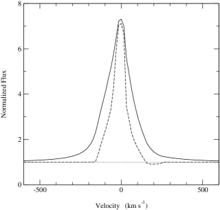
Figure 4: The effect of line broadening on H$\alpha$. A model computed with a damping constant ($\Gamma$), described in Section 3 (solid), is compared with a model with no damping, $\Gamma=0$ (dashed). Both models are computed with $T_{\mathrm{max}}=7500\leavevmode\nobreak\ \mathrm{K}$, $i=55^{\circ}$, and the reference parameters given in Table 1. The two models have similar peak flux levels (around $V\sim 0\leavevmode\nobreak\ \mathrm{km\leavevmode\nobreak\ s^{-1}}$), but the total flux and the EW of the line increased drastically for the model with the damping constant. The broad wings extend to $\sim\pm 800\,\mathrm{km\leavevmode\nobreak\ s^{-1}}$. The redshifted absorption feature seen (very weakly) in the $\Gamma=0$ model is not seen in the model with the broadening.

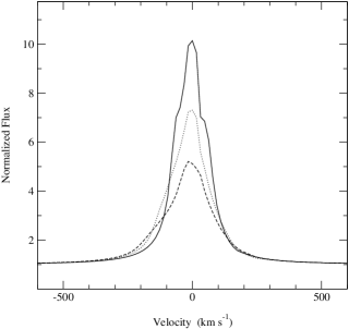
Figure 5: The dependency of the H$\alpha$ profile on inclination ($i$). The profiles are computed with a magnetospheric accretion flow only using the reference parameters given in Table 1 and $T_{\mathrm{max}}=7500\leavevmode\nobreak\ \mathrm{K}$. The solid, dotted, and dashed lines are for $i=10^{\circ}$, $55^{\circ}$, and $80^{\circ}$ respectively. As the inclination becomes larger, the peak flux and the equivalent width of the line become smaller.

Using the reference model parameters (Table 1) for the central star and the magnetosphere, we examine the dependency of H$\alpha$ on the temperature ($T_{\mathrm{max}}$) of the accretion flow and the mass accretion rate ($\dot{M}_{\mathrm{acc}}$), as done by Muzerolle et al. (2001) for H$\beta$. The temperature structure of Hartmann et al. (1994) is adopted here, and the parameter $T_{\mathrm{max}}$ sets the maximum temperature of the accretion streams. We note that here we have computed the hot ring temperature self-consistently, whereas Muzerolle et al. (2001) used a constant hot ring temperature ($8000\,\mathrm{K}$) for most of their models. The accretion luminosity ($L_{\mathrm{acc}}$) for models with $\dot{M}_{\mathrm{acc}}=10^{-7}\,\mathrm{M_{\sun}\,yr^{-1}}$ is about a half of the photospheric luminosity.

H$\alpha$ line profiles for a range of $T_{\mathrm{max}}$ and $\dot{M}_{\mathrm{acc}}$ are presented in Fig. 3. The overall dependency on $T_{\mathrm{max}}$ and $\dot{M}_{\mathrm{acc}}$ is similar to that of Muzerolle et al. (2001). In general, the line strength weakens as the accretion rate and the temperature drop. The red-shifted absorption becomes less visible for the higher accretion rate and higher temperature models as it becomes filled-in by the stronger Stark-broadened line-wing emission.

We demonstrate this effect in Fig. 4, which shows an example for an H$\alpha$ model with $T_{\mathrm{max}}=7500\,\mathrm{K}$ and $\dot{M}_{\mathrm{acc}}=10^{-7}\,\mathrm{M_{\sun}\,yr^{-1}}$, both with and without damping. Although the maximum flux of the model with broadening is almost identical to that of the model with no damping constant ($\Gamma=0$), a significant increase of the line flux in both red and blue wings is seen. The weak red-shifted absorption component (which is a signature of the magnetospheric accretion) is weakened or eliminated by the flux in broadened wing.

Table 2 shows the equivalent width (EW) for the models in Fig. 3. The EWs for half the models fall within the range of EWs ($\sim 3$ to $\sim 160$ Å) measured by Alencar & Basri (2000). The EWs of models with the lowest mass accretion rates fall below the minimum EW observed by Alencar & Basri (2000), while several models would be designated as weak-lined T Tauri stars (WTTS) using the traditional 10 Å cut-off (e.g. Herbig & Bell, 1988). White & Basri (2003) empirically showed that the full width of H$\alpha$ at 10 per cent of its peak flux (10 per cent width) is a better indicator for an accretion than the EW criteria. They proposed that if a T Tauri star shows a 10 per cent width greater than $270\,\mathrm{km\,s^{-1}}$, the star should be a CTTS. The 10 per cent widths of the model H$\alpha$ profiles (Fig. 3) are summarised in Table 3. Using the criteria of White & Basri (2003), half of the models shown in the figure can be classified as CTTS, and the other half as WTTS. However, the profiles corresponding to the WTTS designations have an inverse P-Cygni morphology that is rarely seen in observations (Reipurth et al. 1996 and Section 5.1).

The dependency of the line profile on inclination angle ($i$) is demonstrated in Fig. 5. The model has $T_{\mathrm{max}}=7500\,\mathrm{K}$ and $\dot{M}_{\mathrm{acc}}=10^{-7}\,\mathrm{M_{\sun}\,yr^{-1}}$. The figure shows that the peak (normalised) flux decreases as the inclination angle increases, as does the EW. The line flux and the EWs decrease mainly because (1) the fraction of the accretion stream blocked by the photosphere increases as the inclination increases (c.f. Fig. 1, lower-left part of the accretion stream i.e. $z<0$ and $x<0$), and (2) the fraction of the accretion stream blocked by the inner part of the accretion disc increases as the inclination increases (c.f. Fig. 1, lower-right part of accretion stream i.e. $z<0$ and $x>0$). While the photosphere mostly blocks the blue-shifted part of the stream, the inner disc blocks the red-shifted part. The line EW in Fig. 5 changes from 32 to 21 Å  as the inclination changes from $10^{\circ}$ to $80^{\circ}$, i.e. a fractional change of 0.65. On the other hand, the 10 per cent width of the line changes from 290 to 470 $\mathrm{km\leavevmode\nobreak\ s^{-1}}$; hence, the fractional change is 1.6. A similar EW dependence on inclination angle is found for the models with different magnetospheric temperatures and the mass-accretion rates.

Because of the geometry of the magnetospheric accretion (c.f. Fig. 1) and of the presence of the gas with the highest velocity close to the stellar surface, the highest blue-shifted line-of-sight velocity is seen only at the high inclination angles. For example, the accretion stream close to the photosphere ($\sim 1R_{*}$ above the photosphere) on the upper-left quadrant in Fig. 1 ($x<0$ and $z>0$) will be more aligned with the line-of-sight of an observer in the upper-right quadrant in the same figure ($x>0$ and $z>0$) as the inclination increases. This results in a slight increase in the blue wing flux for a higher inclination model as seen in Fig. 5.

Our models show a blue-shifted line peak and a blueward asymmetry caused by occultation of the accretion flow by the stellar photosphere (see also Hartmann et al. 1994; Muzerolle et al. 2001). However, Alencar & Basri 2000 (see their fig. 9) found a substantial fraction of the observed H$\alpha$ profiles show a red-shifted peak. Furthermore, a recent study by Appenzeller et al. (2005) demonstrated that the equivalent width of H$\alpha$ from CTTS increases as the inclination angle increases. Clearly a magnetospheric accretion only model cannot explain the full properties of the H$\alpha$ profiles in CTTS.

Table 2: Summary of H$\alpha$ equivalent widths (Å) from the magnetospheric accretion flow models shown in Fig. 3. Note that the equivalent widths are positive when the lines are in emission.

$T_{\mathrm{max}}\,\,\left(\mathrm{K}\right)$		$\dot{M}_{\mathrm{acc}}$  $\left(\mathrm{M_{\sun}\,yr^{-1}}\right)$
	$10^{-7}$	$10^{-8}$	$10^{-9}$
$6500$	$17.9$	$0.1$	$0.0$
$7500$	$25.2$	$-0.9$	$-0.5$
$8500$	$68.3$	$6.5$	$-0.7$
$9500$	$98.6$	$52.4$	$1.3$

Table 3: Summary of 10 per cent widths ($\mathrm{km\,s^{-1}}$) from the magnetospheric accretion flow models shown in Fig. 3.

$T_{\mathrm{max}}\,\,\left(\mathrm{K}\right)$		$\dot{M}_{\mathrm{acc}}$  $\left(\mathrm{M_{\sun}\,yr^{-1}}\right)$
	$10^{-7}$	$10^{-8}$	$10^{-9}$
$6500$	$300$	$120$	$100$
$7500$	$360$	$145$	$120$
$8500$	$790$	$330$	$130$
$9500$	$1530$	$520$	$200$

4.2 Disc-wind only models

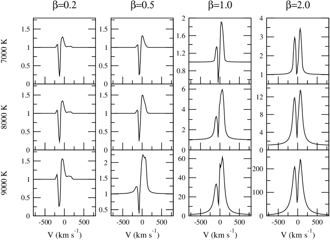
Figure 6: H$\alpha$ profiles computed with the disc-wind only. The wind mass-loss rate is fixed at $\dot{M}_{\mathrm{wind}}=10^{-8}\,\mathrm{M_{\sun}\,yr^{-1}}$, and the line profiles are computed with different combinations of the wind acceleration rate ($\beta$) and isothermal disc-wind temperature ($T_{\mathrm{wind}}$). The wind emission grows as the values of $\beta$ and $T_{\mathrm{wind}}$ increase. The position of the wind absorption moves toward the line centre as $\beta$ becomes larger.

In this section, we examine profiles produced using the disc wind outflow model described in Section 2.3. The parameters used for the central star are as in Section 2.1, and the disc-wind parameters are summarised in Table 4. Although the line is potentially sensitive to the temperature structure of the wind, determination of a self-consistent wind temperature is beyond the scope of this paper. Readers are refereed to Hartmann et al. (1982) in which the wind temperature structure is determined by balancing the radiative cooling rate (assuming optically thin) with the MHD wave heating rate. We pragmatically assume that the wind is isothermal at $T_{\mathrm{wind}}$.

Initially we examine the characteristics of the H$\alpha$ profile as a function of the wind acceleration parameter $\beta$ and the isothermal wind temperature $T_{\mathrm{wind}}$. The mass-loss rate is kept constant at $\dot{M}_{\mathrm{wind}}=10^{-8}\,\mathrm{M_{\sun}\,yr^{-1}}$. Fig. 6 shows the model profiles computed for the wind temperatures between $7000\,\mathrm{K}$ and $9000\,\mathrm{K}$, and those with $\beta$ between $0.2$ and $2.0$, computed at inclination $i=55^{\circ}$. The morphology of the profile exhibited by the model changes from FU-Ori type (c.f. Reipurth et al. 1996) for the models with small $\beta$ to the stronger emission types, which are more commonly seen in the observed H$\alpha$ (c.f. Reipurth et al. 1996), as the value of $\beta$ increases. Classical P Cygni profiles are prominent in the models with lower values of $T_{\mathrm{wind}}$ and $\beta$ (a colder and faster accelerating wind). As the value of $\beta$ increases, the position of the blue-shifted absorption component moves toward the line centre. The blue edge of the absorption component in the fastest accelerating wind ($\beta=0.2$) model is almost at the terminal velocity ($v_{\infty}\sim 160\,\mathrm{km\leavevmode\nobreak\ s^{-1}}$) of the disc wind (c.f. Fig. 2), that for the slowest wind acceleration model ($\beta=2.0$) is located close the line centre ($\sim 20\,\mathrm{km\leavevmode\nobreak\ s^{-1}}$).

The intensity of the emission component increases as $\beta$ increases for a fixed $T_{\mathrm{wind}}$. This is mainly because the density near the photosphere increases as the value of $\beta$ increases (Fig. 2); hence, the emissivity increases. Most of the profiles show a red-ward asymmetry, mainly due to the presence of the classical P-Cygni absorption. However we find that the disc-wind models with the fastest acceleration ($\beta=0.2$ and $0.5$) and viewed at low inclinations, show a strong blue asymmetry due to occultation of the receding half of the outflow by the optically thick disc.

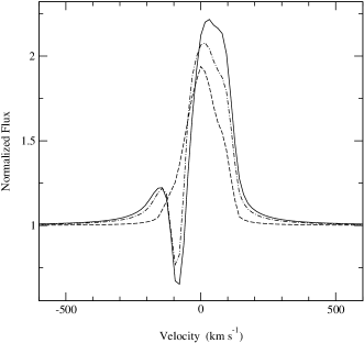
Figure 7: The dependency of the H$\alpha$ profile on the source displacement parameter $d$. The line profiles are computed with the wind parameter $T_{\mathrm{wind}}=9000\mathrm{K}$ and $\beta=0.5$ for $i=55^{\circ}$. The profiles in the figure use $d=2\leavevmode\nobreak\ R_{*}$ (dashed), $7\leavevmode\nobreak\ R_{*}$ (dash-dot) and $22\leavevmode\nobreak\ R_{*}$ (solid). All the other parameters are same as in Fig. 6. As the wind becomes more collimated (larger $d$), the wind emission becomes stronger. The P-Cygni absorption disappears for the model with a small collimation (e.g. $d=2\leavevmode\nobreak\ R_{*}$ case) since the opening angle of the disc wind is larger than the inclination angle.

We now examine the sensitivity of the model profiles to the wind collimation or the source displacement parameter $d$. As we can see from Fig. 1, the disc wind geometry/collimation is determined by $d$ and the wind launching radii ($R_{\mathrm{wi}}$ and $R_{\mathrm{wo}}$). Here, we fix the values of $R_{\mathrm{wi}}$ and $R_{\mathrm{wo}}$ as in Table 4, and inspect the model dependency on $d$ alone. The minimum wind opening angle (measured from the symmetry axis) is given by $\theta_{\mathrm{open}}=\arctan\left(R_{\mathrm{wi}}/d\right)$. Fig. 7 shows the profiles computed for $d=2\leavevmode\nobreak\ R_{*}$, $7\leavevmode\nobreak\ R_{*}$ and $22\leavevmode\nobreak\ R_{*}$ for the inclination angle $i=55^{\circ}$. As the wind becomes more collimated (larger $d$), the wind opening angle becomes smaller and the wind density is enhanced towards the symmetry axis ($z$); hence, the wind emission increases. When the collimation of the wind is small (as in the $d=2\leavevmode\nobreak\ R_{*}$ case), the P-Cygni absorption is absent from the profile because the opening angle of the disc wind is greater than the inclination angle. For the disc wind models presented in Fig. 6, we use $d=22\leavevmode\nobreak\ R_{*}$ in order to have a moderate amount of wind absorption at a moderate inclination angle ($i\sim 60^{\circ}$).

Blandford & Payne (1982) showed that in order to launch a wind from a disc plane magneto-centrifugally, the launching angle ($\theta_{L}$, measured from the equatorial disc plane) must be less than $60^{\circ}$. In our models, the wind launching zone is restricted in between $R_{\mathrm{wi}}<w_{i}<R_{\mathrm{wo}}$ (see Fig. 1 and Table 1) with $R_{\mathrm{wi}}=3\,R_{*}$ and $R_{\mathrm{wo}}=1$ au. This sets the upper limit of the source displacement distance ($d$) to be around $5.2\,R_{*}$ if we want to satisfy the launching angle condition of Blandford & Payne (1982) for all the stream lines in our disc wind model. In the models presented in Fig. 6 (and later in Fig. 9 in next section), we have adopted $d=22\,R_{*}$ instead. This means that some part of the disc wind ($3\,R_{*}<w_{i}<12.7\,R_{*}$) may not be able to be launched from the disc plane according to the model of Blandford & Payne (1982). We have used a larger launching angle or a larger source displacement distance for the following two reasons.

First, we want to simulate a more collimated wind (toward the symmetry axis). Since the stream lines in our simple disc wind are represented by straight lines, the wind never bends toward the symmetry axis ($z$-axis) as the distance from the disc increases unlike the model of Blandford & Payne (1982). We therefore used a larger launching angle to simulate the stream lines in the far field (at a larger distance from the disc plane) in their model. This is an intrinsic problem with approximating the stream lines with straight lines.

Second, the larger source displacement model would provide a greater consistency with the fraction of H$\alpha$ profiles affected by wind absorption seen in observations. According to the observations of Reipurth et al. (1996) and Alencar & Basri (2000), more than 50 per cent of CTTS show wind absorption features in their H$\alpha$ profiles. In our model, if the launching angle is too small ($\theta_{\mathrm{L}}<60^{\circ}$), the wind absorption feature would not be seen or would be very small for profiles computed with $i<60^{\circ}$, as demonstrated in Fig. 7. The situation will however change if the field/stream line is not straight and bending towards the symmetry axis as the wind travels higher above the disc.

In addition to the models given in Figs. 6 and 9, we have computed the models with $d=5\,R_{*}$ (not shown here) which satisfy the wind launching condition of Blandford & Payne (1982) in all parts of the disc wind zone in our model. These models showed that the wind absorption and emission features weaken, but overall morphology dependence of the profiles on the wind temperature and the wind acceleration rate is similar to what we found in the models shown in Figs. 6 and 9. The minimum inclination angle at which the wind absorption becomes important is larger than that of the models with a larger source displacement ($d=22\,R_{*}$) as expected.

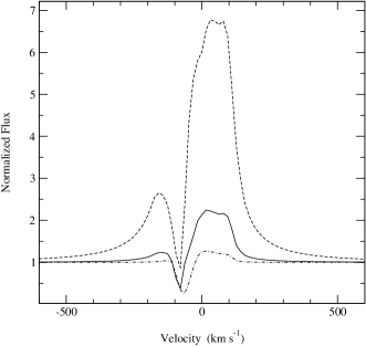
Figure 8: The effect of the wind mass-loss rate. The profiles computed with $\left(T_{\mathrm{wind}},\leavevmode\nobreak\ \beta\right)=\left(9000\mathrm{K},0.5\right)$, and $\dot{M}_{\mathrm{wind}}=2.0\times 10^{-8}\leavevmode\nobreak\ \mathrm{M_{\sun}\,yr^{-1}}$  (dashed), $1.0\times 10^{-8}\leavevmode\nobreak\ \mathrm{M_{\sun}\,yr^{-1}}$  (solid), and $0.5\times 10^{-8}\leavevmode\nobreak\ \mathrm{M_{\sun}\,yr^{-1}}$  (dash-dot) are shown above. With all other parameter fixed, the mass-loss rate behaves as a scaling factor for the wind density (c.f. equation 6).

Finally, the effect of varying the wind mass-loss rate is shown in Fig. 8. With all other parameters fixed, $\dot{M}_{\mathrm{wind}}$ acts as a scaling factor for the wind density (equation 6). The most important process that populates the $n=3$ level is recombination, and therefore the line emissivity varies as the square of the density (assuming that the ionisation fraction remains constant); hence the line is very sensitive to changes in $\dot{M}_{\mathrm{wind}}$. We indeed find that the line flux of the models is approximately proportional to the square of the mass-loss rate.

Table 4: A summary of the reference disc-wind model parameters used in Sections 4.2 and 4.3. See also Section 2.3.

$R_{\mathrm{wi}}$	$R_{\mathrm{wo}}$	$\dot{M}_{\mathrm{wind}}$	$p$	$f$	$R_{\mathrm{s}}$
$\left[R_{*}\right]$	$\left[\mathrm{au}\right]$	$\left[\mathrm{M_{\sun}\,yr^{-1}}\right]$	$[-]$	$[-]$	$\left[R_{*}\right]$
$3.0$	$1.0$	$10^{-8}$	$-7/2$	$2.0$	$30$

4.3 Disc-wind-magnetosphere hybrid models

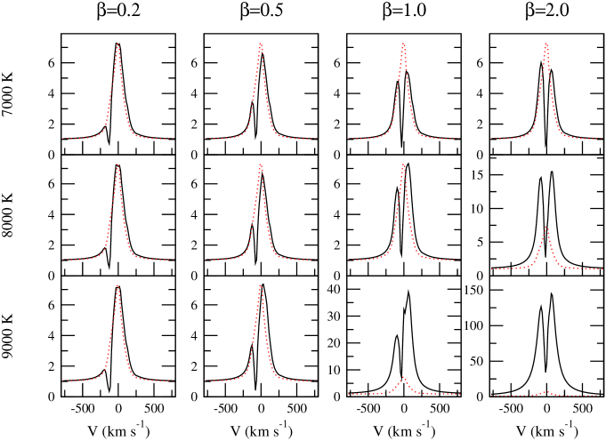
Figure 9: The disc-wind-magnetosphere hybrid model. These models (solid lines) have the same parameters as Fig. 6, but also include the magnetospheric accretion flow ($T_{\mathrm{\max}}=7500\leavevmode\nobreak\ \mathrm{K}$ and $\dot{M}_{\mathrm{acc}}=10^{-7}\,\mathrm{M_{\sun}\,yr^{-1}}$). While the emission from the magnetosphere dominates for the models with smaller $\beta$ and $T_{\mathrm{wind}}$, the emission from the wind dominates the profiles for models with larger $\beta$ and $T_{\mathrm{wind}}$. The contribution of the magnetosphere can be judged from the profiles computed with the magnetosphere only (dotted lines).

We now consider models computed with a combination of the disc-wind and magnetospheric accretion components. The parameters used for the magnetosphere are same as in Fig. 5 (with $i=55^{\circ}$ ), and the mass-loss rate of the disc wind is $\dot{M}_{\mathrm{wind}}=10^{-8}\,\mathrm{M_{\sun}\,yr^{-1}}$ (i.e. $\mu=\dot{M}_{\mathrm{wind}}/\dot{M}_{\mathrm{acc}}=0.1$). Fig. 9 shows the models profiles computed (at $i=55^{\circ}$) using the same ranges of the disc-wind temperature and wind acceleration parameter as in the previous cases.

As in the disc-wind only models (Fig. 6), the location of the absorption component moves toward the line centre as the value of $\beta$ increases. The figure shows that in the models with smaller $\beta$ and $T_{\mathrm{wind}}$, the line emission from the magnetosphere dominates, while this situation reverses for the models with larger $\beta$ and $T_{\mathrm{wind}}$. The model with $\left(T_{\mathrm{wind}},\,\beta\right)=\left(9000\,\mathrm{K},\,2.0\right)$ results in an H$\alpha$ profile that is far too strong to be compatible with observations (Reipurth et al. 1996; Alencar & Basri 2000); however, the lower mass-loss rate models (while keeping $\mu$ constant) produce profiles with the line strengths comparable to observations (c.f. Appendix A). Although the models in Fig. 9 are computed with limited ranges of $T_{\mathrm{wind}}$, $\beta$ and a fixed $i$, the resulting profiles exhibit a wide variety of line profile shapes, many of which are similar to the types of H$\alpha$ profiles seen in the observations (c.f. Reipurth et al. 1996).

In order to quantify the relative contributions of the wind emission and the magnetosphere, we have computed the ratio of the EW of the hybrid model in Fig. 9 to the EW of the magnetosphere only model (Table 5). This ratio falls below 1.0 when the wind only contributes to the line absorption, but not to the emission. In some models (e.g. with $T_{\mathrm{wind}}=8000\,\mathrm{K}$ and $\beta=2.0$), the contribution of the wind to the EW is much larger than that of the magnetosphere (EW ratio is 3.2). This clearly demonstrates that the difficulty of using the EW of H$\alpha$ alone as an accretion measure. We have also seen in Fig. 6 that disc wind models without a magnetosphere can produce an H$\alpha$ line with significantly large EW.

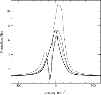
Figure 10: The effect of the mass-loss rate to mass-accretion rate ratio ($\mu=\dot{M}_{\mathrm{wind}}/\dot{M}_{\mathrm{acc}}$). The H$\alpha$ profile computed with only the magnetospheric accretion (thick solid) is compared to the disc-wind-magnetosphere hybrid models for $\mu=$ 0.05 (dash-dot), 0.1 (solid) and 0.2 (dash). The magnetosphere used here has $T_{\mathrm{max}}=7500\,\mathrm{K}$ and $\dot{M}_{\mathrm{acc}}=10^{-7}\,\mathrm{M_{\sun}\,yr^{-1}}$. The temperature and the acceleration parameter of the disc wind are $T_{\mathrm{wind}}=9000\,\mathrm{K}$ and $\beta=0.5$ respectively. All the models are computed with the inclination angle $i=55^{\circ}$. As $\mu$ increases the emission component becomes stronger and the wings becomes broader, as expected. The absorption component is relatively insensitive to the value of $\mu$ in this example. The wide range of $\mu$ reasonably reproduces the profiles similar to ones seen in observations (e.g. Reipurth et al. 1996).

An examination of the profiles in Figs. 6 and 9 reveals some problems with uniqueness that must inevitably occur when trying to assign an individual profile as wind or accretion dominated i.e. very similar profiles may arise from very different circumstellar geometries. For example, the disc-wind only model with $\left(T_{\mathrm{wind}},\,\beta\right)=\left(8000\,\mathrm{K},\,1.0\right)$ in Fig. 6 and the accretion dominated model with $\left(T_{\mathrm{wind}},\,\beta\right)=\left(9000\,\mathrm{K},\,0.5\right)$ in Fig. 9 give very similar profiles.

The effect of changing the ratio of the wind mass-loss rate to mass-accretion rate ($\mu=\dot{M}_{\mathrm{wind}}/\dot{M}_{\mathrm{acc}}$) is demonstrated in Fig. 10. With a fixed value of mass-accretion rate ($\dot{M}_{\mathrm{acc}}=10^{-7}\,\mathrm{M_{\sun}\,yr^{-1}}$), the mass-loss rate is varied. The figure shows that as $\mu$ increases the P-Cygni absorption deepens only slightly, and the position of minimum flux in the absorption trough appears to remain at same location. On the other hand, the flux peak increases and the line wings become stronger as $\mu$ increases. Although MHD models suggest (e.g. Königl & Pudritz 2000) that $\mu\sim 0.1$, the figure suggest that models with a relatively wide range of $\mu$ (e.g. between 0.05 and 0.2 in this case) produce profiles similar to observations.

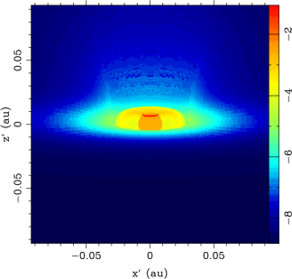
Figure 11: An H$\alpha$ image of the disc-wind hybrid model viewed at an inclination of 80^∘. The false-colour scale shows logarithmic (base 10) surface brightness (arbitrary units) and the axes are linear dimensions in au. The parameters used for the magnetosphere are as the reference model in Table 1. The wind temperature of $T_{\mathrm{max}}=7000\leavevmode\nobreak\ \mathrm{K}$ and the wind acceleration parameter $\beta=1.0$ are adopted here.

By inspecting the model H$\alpha$ images computed (Fig. 11), we have found that the extent of the H$\alpha$ emission region is relatively small (i.e. $h\sim 0.1\,\mathrm{au}$ or $10\,R_{*}$ where $h$ is the vertical distance from the disc) when compared to the spectro-astrometric observations of Takami et al. (2003) for RU Lup and CS Cha which show 1–5 au scale outflows. In our model, the wind emission flux drops by $\sim 10^{4}$ by the time the wind reaches $h\approx 0.1\,\mathrm{au}$. The extent of the line emission region becomes slightly larger ($\sim 0.4$ au) if a slower wind acceleration rate (e,g, $\beta=4$) is used. The discrepancy between the observations and the model is perhaps caused by the lack of the material connecting the disc wind to a collimated jet in our model, which may be excited by alternative heating mechanism (e.g. shocks) thus producing observable H$\alpha$ emission at large distances from the central object.

Table 5: The ratio of the line equivalent width (EW) of the disc-wind magnetosphere hybrid models in Fig. 9 to the EW of the magnetosphere only model.

$T_{\mathrm{max}}\,\,\left(\mathrm{K}\right)$		$\beta$
		$0.2$	$0.5$	$1.0$	$2.0$
$7000$		$1.1$	$.94$	$.89$	$.96$
$8000$		$1.1$	$.92$	$1.2$	$3.2$
$9000$		$1.0$	$1.1$	$7.5$	$36.$

5 Discussion

5.1 The morphological classification scheme proposed by Reipurth et. al (1996)

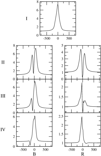
Figure 12: Sample H$\alpha$ model profiles which characterise the classification scheme of Reipurth et al. (1996). The combination of magnetospheric accretion flow, the accretion disc, and the disc-wind can reproduce the wide range of H$\alpha$ profiles seen in observations. The model parameters used for each profile along with short comments are given in Table 6. The horizontal axes are velocities in $\mathrm{km\leavevmode\nobreak\ s^{-1}}$, and the vertical axes are normalised flux.

Reipurth et al. (1996) proposed a two-dimensional classification of H$\alpha$ emission profiles of T Tauri stars and Herbig Ae/Be stars. Their classification scheme contains four classes (I, II, III and IV) differentiated by the ratio of the secondary-to-primary emission components in the profiles. Each class is divided into two sub-classes (B and R) which depends whether the secondary peak is on the blue or red side of the primary peak. Readers are referred to Fig. 4 of their paper. Fig. 12 shows sample model profiles which are classified according to the definition of Reipurth et al. (1996). The combination of the disc wind, magnetospheric accretion flow, and the accretion disc can reproduce all the classes of the profiles seen in observations. The corresponding parameters of the disc-wind-magnetosphere hybrid model used to reproduce the profiles in the figure are summarised in Table 6 along with brief comments on possible physical conditions which lead to the profiles in each class. Below we discuss the Reipurth scheme in the context of our models parameters. Readers are referred to Appendix A for the complete model profiles used in this discussion. Although in general H$\alpha$ in the spectra of CTTS shows a significant amount of variablity, which may in some cases be induced by the rotational motion of an inclined magnetosphere (e.g. Johns & Basri 1995; Bouvier et al. 2003), we restrict our discussion in this section to the axi-symmetric case only.

Type I: Reipurth et al. (1996) found that Type I profiles (symmetric around line centres) constituted 26 per cent of the 43 CTTS H$\alpha$ profiles in their sample, making it the second most common morphological type. We find that Type I profiles are dominated by magnetospheric emission at rates in excess of $\approx 10^{-8}\,\mathrm{M_{\sun}\,yr^{-1}}$. Type I profiles appear at a wide range of inclinations (Fig. 5). An object that displays a Type I profile may have relatively weak disc wind, but in this case it must be viewed from the pole (in order that no wind material is seen projected against the stellar photosphere).

Type II-B: These profiles have a secondary blue peak that is in excess of half the strength of the primary peak, and comprised 16 per cent of the Reipurth sample. We find that Type II-B profiles only occur at medium to high inclinations, and for systems with mass accretion rates of $\approx 10^{-7}\,\mathrm{M_{\sun}\,yr^{-1}}$. If the system is viewed at high inclination, a Type II-B profile implies a fast wind acceleration, and conversely a moderate inclination angle suggests a more modest wind acceleration.

Type II-R: These profiles are characterised by a secondary red peak that is in excess of half the strength of the primary peak. They are approximately as common as the Type II-B lines. For the $\dot{M}_{{\rm acc}}=10^{-7}\,\mathrm{M_{\sun}\,yr^{-1}}$ a switch from Type II-B profiles to Type II-R occurs when the inclination angle changes from $55^{\circ}$ to $80^{\circ}$. This profile type is also seen at lower mass-accretion rates, but typically only in the models with the slowest accelerating winds. It is perhaps unsurprising that the Type II-B and Type II-R profiles are equally common, since (in general) the split between the profile types results from a geometrical (viewing angle) effect rather than a marked difference in physical parameters (mass accretion rate, wind acceleration etc).

Type III-B: Profiles with a blue secondary peak that is less than half the strength of the primary peak are classified as Type III-B. This type of profile is the most common in the Reipurth sample, comprising 14 out of 43 (33 per cent) CTTS. We find Type III-B profiles only in our $\dot{M}_{{\rm acc}}=10^{-7}\,\mathrm{M_{\sun}\,yr^{-1}}$ models. A fast wind acceleration and a moderate inclination are necessary, or a slower accelerating wind viewed pole-on. We do not see this profile type in our high inclination models. Although Type III-B profiles do not occur at $\dot{M}_{\mathrm{acc}}=1.0\times 10^{-8}\,\mathrm{M_{\sun}\,yr^{-1}}$, we have examined the intermediate case of $\dot{M}_{\mathrm{acc}}=3\times 10^{-8}\,\mathrm{M_{\sun}\,yr^{-1}}$, which may represent a typical T Tauri mass accretion rate (Gullbring et al. 1998; Calvet et al. 2004). We find that the models with fast accelerating, high temperature winds do display Type III-B profiles. It is clear that our model, as it stands, requires above-average (but perhaps not atypical) mass-accretion rates in order to produce Type III-B profiles. It is less clear whether the 14 Type III-B objects found by Reipurth et al. (1996) constitute the highest mass-accretion rate objects in their sample: the average EW for T Tauri stars with Type III-B profiles is 64 Å, which is in the top quartile of their complete T Tauri star sample, perhaps indicating that Type III-B profiles are associated with high EWs, and therefore strong mass-accretion.

Type III-R: This profile type has a red secondary peak that is less than half the strength of the primary peak, and only one object with this type of profile was observed in the Reipurth sample (SZ Cha). We are able to reproduce this profile type, but only using a very narrow range of parameter space. In fact there are no Type III-R profiles in our model grid, but we obtain one by ‘tweaking’ the magnetospheric temperature, and using an inclination ($85^{\circ}$) sufficient that the disc starts to obscure the central H$\alpha$ emission. For completeness, the final model parameters we used to achieve the profiles are: very high inclination, $T_{\mathrm{max}}\sim 8300\,\mathrm{K}$, and $\dot{M}_{\mathrm{acc}}\sim 10^{-8}\,\mathrm{M_{\sun}yr^{-1}}$. It is interesting that the most infrequently observed profile type was in fact the most difficult for us to reproduce. It appears that this profile morphology requires some obscuration effects by the dust disc, and therefore a high inclination; this naturally explains the rarity of the profile in the observations.

Type IV-B: This profile classification is the classical P-Cygni, in which the blue-shifted absorption component has a sufficient velocity to be present beyond the emission line wing. It occurs infrequently in observations (7 per cent of the Reipurth sample). No Type IV-B profiles were produced in our model grid, since the blue wing of the magnetosphere has generally such a large extent that it always exceeds the projected wind terminal velocity, and thus the bluemost extent of the absorption component. Only by running a model with a larger terminal velocity or with a smaller magnetospheric temperature, were we able to achieve a classical P-Cygni shape. We suspect that the disc-wind geometry is not the best kinematic model for producing this morphology. A more straightforward explanation lies with a bipolar flow, viewed along its axis, or even a simple spherical wind.

Type IV-R: This is the inverse P-Cygni profile type, and only occurs in about 5 per cent of H$\alpha$ profiles. Type IV-R profiles occur very infrequently in our hybrid model grid, with only the lowest mass-accretion rate models viewed at high inclination showing the characteristic shape (although using the EW criterion these models would not be classified as CTTS). The inverse P-Cygni profile requires that the observer view the hot accretion footprints through the fast moving magnetospheric accretion flow, and this means that the inclination angle is restricted to small range. We can reproduce Type IV-R profiles more readily if we adopt a cooler magnetospheric temperature than indicated by the accretion-rate/temperature relationship presented by Muzerolle et al. (2001). The restriction in the inclination angle mentioned above would be relaxed if the axis of the magnetosphere was tilted with respect to the rotational axis since the line-of-sight from an observer to the hot rings will pass through different parts of the magnetosphere as the rotational phase changes.

Table 6: The summary of model parameters for the profiles in Fig. 12 and brief comments. The temperatures are in $10^{3}\,\mathrm{K}$. $\dot{M}_{\mathrm{acc}}$ and $\dot{M}_{\mathrm{wind}}$ are in $\mathrm{M_{\sun}\,yr^{-1}}$.

Class	$i$	$\dot{M}_{\mathrm{acc}}$	$T_{\mathrm{max}}$	$\dot{M}_{\mathrm{wind}}$	$T_{\mathrm{wind}}$	$\beta$	Comment
I	$55^{\circ}$	$10^{-7}$	$7.5$	$-$	$-$	$-$	Accretion dominated. Wide range of inclination.
II-B	$55^{\circ}$	$10^{-7}$	$7.5$	$10^{-8}$	$8.0$	$1.0$	Wide range of wind acceleration rates. Mid–high inclination.
II-R	$80^{\circ}$	$10^{-7}$	$7.5$	$10^{-8}$	$7.0$	$2.0$	Slow wind acceleration rate. High inclination.
III-B	$55^{\circ}$	$10^{-7}$	$7.5$	$10^{-8}$	$9.0$	$0.5$	Fast wind acceleration rate. Mid inclination.
III-R	$85^{\circ}$	$10^{-8}$	$8.2$	$10^{-9}$	$6.0$	$1.0$	Mid wind acceleration rate. Very high inclination.
IV-B	$30^{\circ}$	$10^{-7}$	$5.5$	$10^{-8}$	$6.0$	$0.2$	Fast wind acceleration rate. Mid–high inclination.
IV-R	$55^{\circ}$	$10^{-9}$	$9.5$	$-$	$-$	$-$	Accretion dominated. Low mass-accretion rate. Mid inclination.

5.2 The inclination dependence of H$\alpha$ profiles

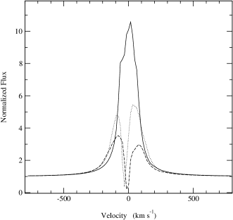
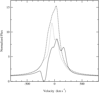
Figure 13: The dependence of the H$\alpha$ model profiles on the inclination angle. The profiles computed at $i=10^{\circ}$ (solid line), $55^{\circ}$ (dotted line) and $80^{\circ}$ (dashed line) using (1) the disc-wind-magnetosphere hybrid model (left; c.f. Section 4.2) and (2) the disc, stellar wind, magnetosphere hybrid model (right panel; c.f. Fig. 14). The parameters used for the magnetosphere are same for the both models, i.e. $T_{\mathrm{max}}=7500\leavevmode\nobreak\ \mathrm{K}$ and $\dot{M}_{\mathrm{acc}}=10^{-7}\leavevmode\nobreak\ \mathrm{M_{\sun}\leavevmode\nobreak\ yr^{-1}}$. The isothermal wind temperature and the wind acceleration parameter used in (1) are $T_{\mathrm{wind}}=7000\leavevmode\nobreak\ \mathrm{K}$ and $\beta=1.0$, and those in (2) are $T_{\mathrm{wind}}=9000\leavevmode\nobreak\ \mathrm{K}$ and $\beta=1.0$ respectively. The wind mass-loss rate used in both models is $\dot{M}_{\mathrm{wind}}=10^{-8}\leavevmode\nobreak\ \mathrm{M_{\sun}\leavevmode\nobreak\ yr^{-1}}$ . All the other parameters are same as in Sections 4.3 and 4.2.

Recently, Appenzeller et al. (2005) have shown that the EW of the observed H$\alpha$ from CTTS is inclination dependent, with the EW increasing as the inclination angle increases. Next, we will examine whether the hybrid model is consistent with the inclination dependency found in the observation. The left-hand panel in Fig. 13 shows the profiles computed with the disc-wind, magnetosphere hybrid model (Section 4.2) at inclination angles $i=10^{\circ}$, $55^{\circ}$ and $80^{\circ}$. The magnetospheric accretion component uses the parameters used as the reference model (Table 1). The figure shows that the absorption feature becomes stronger as the inclination increases, mainly because of the geometrical configuration. The optical depth to the observer becomes larger as the inclination angle increases, since the density of the disc wind increases towards the equatorial plane – as a result, the EW becomes smaller as the inclination angle increases: 41, 27, and 19 Å  for $i=10^{\circ}$, $55^{\circ}$, and $80^{\circ}$ respectively. This is a robust result, and is insensitive to the adopted wind parameters. Recall that this is the same EW/inclination dependency as the magnetosphere only models (Fig. 5).

Clearly the inclination dependency of the line strength is in contradiction with the Appenzeller et al. (2005) result, and thus merits further investigation. In the previous sections, we have considered H$\alpha$ line formation in a disc wind, which mimics the density distribution of the magneto-centrifugal launched jet models (e.g. Krasnopolsky et al. 2003). The density in this model is more concentrated toward the equatorial plane in the region where the line emissivity is highest, although further out the material becomes collimated into a bipolar jet, this would not contribute significantly to the line emission in our models.

As an alternative, we consider a wind model in which the outflow density increases towards the pole, rather than the equator. In this model, the disc-wind is replaced by a stellar wind, propagating only in the radial direction, accelerating under the classical beta-velocity law (c.f. Castor & Lamers, 1979) i.e. $v_{r}\left(\ r\right)=v_{\infty}\left(1-R_{*}/r\right)^{\beta}$ where $v_{\infty}$ and $R_{*}$ are the wind terminal velocity and the stellar radius respectively. $\beta$ is the wind acceleration parameter similar to the one seen in the disc-wind model (c.f. equation 5). The wind emerges from the stellar surface, but restricted to be within $\sim 30^{\circ}$ from the symmetry axis hence forming the cone-shaped regions both above and below the poles. The density is computed from assuming a constant mass-loss rate per unit area over the stellar surface, requiring mass-flux conservation, and using the beta velocity law above. The schematic of the model configuration is shown in Fig. 14. Again, we assume the wind temperature ($T_{\mathrm{wind}}$) is isothermal for simplicity. This model configuration is motivated by the recent study by Matt & Pudritz (2005) who demonstrated that a stellar wind along open magnetic field lines originating from the star may cause significant spin-down torque.

The right-hand panel in Fig. 13 shows H$\alpha$ profiles computed using the alternative model at the same inclination angles used for the disc-wind-magnetosphere hybrid model. The mass-loss rate of the stellar wind in this model is $10^{-8}\,\mathrm{M_{\sun}\,yr^{-1}}$, which is the same as the mass-loss rate used in the disc-wind magnetosphere hybrid model in the same figure. In both models, the mass-accretion rate of $10^{-7}\,\mathrm{M_{\sun}\,yr^{-1}}$ is used. The wind acceleration parameter ($\beta$) and the wind temperature ($T_{\mathrm{wind}}$) used here are $1.0$ and $9000\,\mathrm{K}$ respectively. All the other parameters are the same as in the disc-wind magnetosphere model. With this set of $\beta$ and $T_{\mathrm{wind}}$, the wind emission is significantly larger than the emission from the magnetosphere. Because of the geometry of the wind, the P-Cygni absorption feature weakens as the inclination increases: the optical depth of the wind is much higher in the polar direction. For the same reason, the EW of the line increases as the inclination increases, as clearly seen in the figure. Specifically the values are 54, 69, and 98 Å  for $i=10^{\circ}$, $55^{\circ}$, and $80^{\circ}$ respectively. This inclination dependency of EW is seen in the models with wide ranges of $\beta$ and $T_{\mathrm{wind}}$, provided that the wind emission of the model is dominating the emission from magnetosphere. A similar inclination dependency of EW is found for lower wind mass-loss rate models (e.g. $\dot{M}_{\mathrm{wind}}=10^{-9}\,\mathrm{M_{\sun}\,yr^{-1}}$) while keeping $\mu=0.1$.

The Appenzeller et al. (2005) study used just 12 objects, and a significantly greater sample should be investigated before firm conclusions are drawn. However our models indicate a significant difference in the inclination dependence of the line morphology which may be simply tested against observation. For example, one possible way to distinguish the two different wind models is to examine the profile shape of a CTTS which is known to be viewed close to pole-on (e.g. a CTTS with a very low $v\sin i$). If the profile contains a prominent blue-shifted absorption component (e.g. Type IV-B), the system is more likely to be associated with the bipolar stellar wind type of outflow, and not with the disc-wind. In reality, however, the two types of winds may be present in the same object, in a similar fashion to that seen in the models of Drew, Proga & Stone (1998) and Matt & Pudritz (2005). In these models, the fast stellar wind is present in the polar directions, while at the same time a slower, denser disc-wind is present near the equatorial plane.

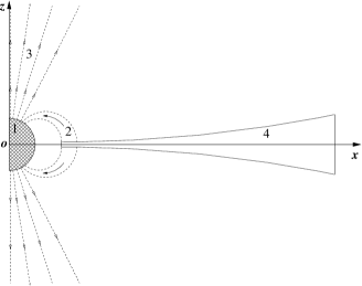
Figure 14: The alternative outflow model. This model replaces the disc-wind with a stellar wind. The wind is launched from the stellar surface, and is limited to cones with opening angles of $\sim 30^{\circ}$. The system consists of four components: (1) the continuum source located at the origin $\left(o\right)$ of the cartesian coordinates $\left(x,y,z\right)$ – the $y$-axis is into the paper, (2) the magnetospheric accretion flow, (3) the stellar wind outflow, and (4) the accretion disc. The density distribution is symmetric around the $z$-axis.

6 Conclusions

We have presented disc-wind-magnetosphere hybrid radiative transfer models for classical T Tauri stars, and detailed studies of the H$\alpha$ formation from their complex circumstellar environment. We found that the hybrid model can reproduce the wide variety of profile seen in observations (Figures 3, 6, 9 and 12).

Using the model results, we examined the H$\alpha$ spectroscopic classification proposed by Reipurth et al. (1996), and discussed the basic physical conditions that reproduce the profiles in each classified type (Section 5.1). Using the different combinations of the inclination ($i$), the mass-loss to mass-accretion rate ratio ($\mu$) and the wind acceleration rate ($\beta$), our radiative transfer model was able to produce all 7 classes of profiles defined in Reipurth et al. (1996).

One potential free parameter of our models is the ratio of mass-loss rate to mass-accretion rate ($\mu$). Most MHD simulations predict a value of $\mu=0.1$ (c.f. Königl & Pudritz 2000), and we have adopted this figure for most of our models. The success of our profile in matching observations is therefore encouraging, and provides support for this canonical value of $\mu$. We have computed sample models with other values of $\mu$, (Fig. 10) and find that models with $0.05<\mu<0.2$ are still consistent with observations. Wind-only or magnetosphere-only models may be representative of individual line profiles, but neither can explain the complete Reipurth classification scheme – even magnetosphere dominated profiles (Type I) can be readily explained by the hybrid model with $\mu=0.1$.

Unfortunately, the dependency of the line equivalent width on the inclination angle predicted by the disc-wind-magnetosphere hybrid model does not agree with the trend seen the observations of Appenzeller et al. (2005). We may appeal to the small sample size of their study (12 objects) to question the validity of the EW effect, but we have also considered an alternative model in which the disc-wind is replaced by a biconical stellar wind, and have found that this alternative wind model can reproduce the line equivalent width dependency on the inclination (Fig. 13). However, MHD simulations predict that bipolar or jet-like flows in CTTS are always accompanied by a disc-wind originating near the star: the actual situation therefore is likely to be a combination of the two flows.

Although we have concentrated on CTTS here, the hybrid model is equally applicable to pre-main-sequence stars across the mass spectrum. Herbig Ae/Be star profiles are equally diverse, and whilst many of the profiles are indicative of a wind (Finkenzeller & Mundt 1984) some lines may be explained by magnetospheric accretion alone (e.g. Muzerolle et al. 2005). One possible advantage in applying the hybrid model to the Herbig Ae/Be systems is the growing observational data probing the line formation region and inner disc using techniques such as spectro-astrometry (e.g. Baines et al., 2005), spectropolarimetry (e.g. Vink et al., 2005a) and interferometry (e.g. Monnier et al., 2005). These high-resolution techniques may aid model fitting of individual objects by constraining some of the model parameters, in particular the inclination.

Velocity broadened, asymmetric H$\alpha$ profiles in brown dwarfs (BDs) are used as an indicator of ongoing magnetospheric accretion, and the same models that are used for CTTS are applied to these systems in order to determine mass-accretion rates (e.g. Lawson, Lyo & Muzerolle 2004; Muzerolle et al. 2005). The line profiles however display the same wide variety of morphologies as the CTTS and Herbig Ae/Be stars (although we note as yet no BD profile has been observed with red-shifted absorption). It is natural to assume that the same physics applies in these low mass objects, and that a hybrid model may be more successful in fitting these profiles, and will give greater insight into the circumstellar kinematics.

There are several avenues of future work to consider. Here we have adopted a simple analytical form for the accretion and outflow velocity and density structure. A more self-consistent approach would be to use the results of MHD simulations as an input to the radiative-transfer modelling. The thermodynamics of the circumstellar gas needs to be examined (c.f. Hartmann et al. 1994; Martin 1996) and also computed self-consistently with the radiation field used in the radiative-transfer, a process that would decrease the free parameters of the model. We intend to calculate other observables from the model that may be compared with observation and should provide further constraints. The line polarisation signature, which arises from scattering of line and continuum photons in the circumstellar dust, encodes both dynamical and geometric information, such as the size of the inner disk radius (e.g. Vink et al. 2005b: Vink et al. 2005a). Spectro-astrometry may provide information on the system’s inclination, and the geometry of the outflow on large scales (e.g. Takami et al. 2003: Baines et al. 2005). Interferometry also provides information on inner disc radii and inclinations, although currently only for the Herbig Ae/Be stars.

We have concentrated on the formation of the H$\alpha$ line, because it is the best studied CTTS emission line. However it is clear that simultaneous fitting of several emission line profiles should provide much stronger constraints. In particular it appears that the near-IR hydrogen lines (Pa$\beta$ and Br$\gamma$) are less affected by outflows than H$\alpha$. One could therefore use these lines to constrain the mass-accretion rate, and use H$\alpha$ to obtain the mass-loss rate. A potential pitfall is the significant temporal variability that all CTTS show in their emission lines; the observational data on a particular object must be co-temporaneous.

Appendix A H$\alpha$ atlas of the disc-wind-magnetosphere hybrid model

Here we present our H$\alpha$ model line profile grid computed using the disc-wind-magnetosphere hybrid model in Section 4.3. All the models use the reference parameters for the magnetospheric geometry and the photosphere as given in Table 1 in the main text. The ratio ($\mu$) of the mass-loss rate to mass-accretion rate is fixed to 0.1 for all the models. Three sets of model profiles, each with a different mass-accretion rate, are presented here: (1) $\dot{M}_{\mathrm{acc}}=10^{-7}\,\mathrm{M_{\sun}\,yr^{-1}}$ (Fig. 15), (2) $\dot{M}_{\mathrm{acc}}=10^{-8}\,\mathrm{M_{\sun}\,yr^{-1}}$ (Fig. 16), and (3) $\dot{M}_{\mathrm{acc}}=10^{-9}\,\mathrm{M_{\sun}\,yr^{-1}}$ (Fig. 17). The temperatures of the magnetospheres used for (1), (2) and (3) are $7500\,\mathrm{K}$, $8500\,\mathrm{K}$ and $9500\,\mathrm{K}$ respectively. The profiles are presented for the inclination angles of $10^{\circ}$, $55^{\circ}$, and $80^{\circ}$. The disc-wind geometry used to compute these profiles are the same as in Section 4.3. These profiles are available electrically at http://www.astro.ex.ac.uk/people/rk/profiles.

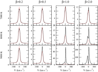
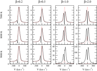
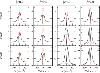
Figure 15: An H$\alpha$ atlas of the disc-wind-magnetosphere hybrid model with $\dot{M}_{\mathrm{acc}}=10^{-7}\,\mathrm{M_{\sun}\,yr^{-1}}$ and $\dot{M}_{\mathrm{wind}}=10^{-8}\,\mathrm{M_{\sun}\,yr^{-1}}$. Profiles are presented for inclinations of $10^{\circ}$ (top figure), $55^{\circ}$ (middle figure), and $80^{\circ}$ (bottom figure). For each inclination, 12 profiles are given, for three different values of the wind temperature, and four different values of the wind acceleration parameter $\beta$. The contribution of the magnetosphere can be judged from the profiles computed with the magnetosphere only (dotted lines).

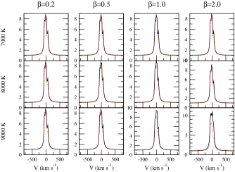
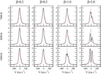
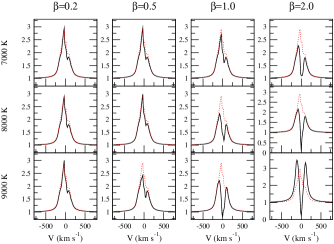
Figure 16: As for Fig. 15 except $\dot{M}_{\mathrm{acc}}=10^{-8}\,\mathrm{M_{\sun}\,yr^{-1}}$ and $\dot{M}_{\mathrm{wind}}=10^{-9}\,\mathrm{M_{\sun}\,yr^{-1}}$.

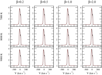
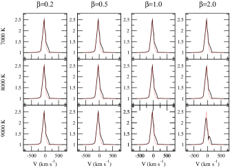
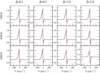
Figure 17: As for Fig. 15 except $\dot{M}_{\mathrm{acc}}=10^{-9}\,\mathrm{M_{\sun}\,yr^{-1}}$ and $\dot{M}_{\mathrm{wind}}=10^{-10}\,\mathrm{M_{\sun}\,yr^{-1}}$.

References

- Alencar & Basri (2000) Alencar S. H. P., Basri G., 2000, AJ, 119, 1881
- Alencar et al. (2005) Alencar S. H. P., Basri G., Hartmann L., Calvet N., 2005, A&A, 440, 595
- Anders & Grevesse (1989) Anders E., Grevesse N., 1989, Geochim. cosmochim. Acta, 53, 197
- Appenzeller et al. (2005) Appenzeller I., Bertout C., Stahl O., 2005, A&A, 434, 1005
- Appenzeller & Mundt (1989) Appenzeller I., Mundt R., 1989, A&AR, 1, 291
- Baines et al. (2005) Baines D., Oudmaijer R., Porter J., Pozzo M., 2005, preprint (astro-ph/0512534)
- Bertout et al. (1988) Bertout C., Basri G., Bouvier J., 1988, ApJ, 330, 350
- Blandford & Payne (1982) Blandford R. D., Payne D. G., 1982, MNRAS, 199, 883
- Bouvier et al. (2003) Bouvier J. et al., 2003, A&A, 409, 169
- Burrows et al. (1996) Burrows C. J. et al., 1996, ApJ, 473, 437
- Calvet & Gullbring (1998) Calvet N., Gullbring E., 1998, ApJ, 509, 802
- Calvet et al. (2004) Calvet N., Muzerolle J., Briceño C., Hernández J., Hartmann L., Saucedo J. L., Gordon K. D., 2004, AJ, 128, 1294
- Camenzind (1990) Camenzind M., 1990, Reviews of Modern Astronomy, 3, 234
- Castor et al. (1975) Castor J. I., Abbott D. C., Klein R. I., 1975, ApJ, 195, 157
- Castor & Lamers (1979) Castor J. I., Lamers H. J. G. L. M., 1979, ApJS, 39, 481
- Chiang & Goldreich (1997) Chiang E. I., Goldreich P., 1997, ApJ, 490, 368
- Collier Cameron & Campbell (1993) Collier Cameron A., Campbell C. G., 1993, A&A, 274, 309
- Draine & Lee (1984) Draine B. T., Lee H. M., 1984, ApJ, 285, 89
- Drew et al. (1998) Drew J. E., Proga D., Stone J. M., 1998, MNRAS, 296, L6
- Edwards et al. (1987) Edwards S., Cabrit S., Strom S. E., Heyer I., Strom K. M., Anderson E., 1987, ApJ, 321, 473
- Edwards et al. (1994) Edwards S., Hartigan P., Ghandour L., Andrulis C., 1994, AJ, 108, 1056
- Finkenzeller & Mundt (1984) Finkenzeller U., Mundt R., 1984, A&AS, 55, 109
- Frank et al. (2002) Frank J., King A., Raine D. J., 2002, Accretion Power in Astrophysics, 3rd edn. Cambridge Univ. Press, Cambridge, p. 398
- Ghosh et al. (1977) Ghosh P., Pethick C. J., Lamb F. K., 1977, ApJ, 217, 578
- Grevesse & Noels (1993) Grevesse N., Noels A., 1993, in Prantzos N., Vangioni-Flam E., Casse M., eds, Origin and Evolution of the Elements, Cambridge Univ. Press, Cambridge, p. 15
- Gullbring et al. (1998) Gullbring E., Hartmann L., Briceno C., Calvet N., 1998, ApJ, 492, 323
- Gullbring et al. (2000) Gullbring E., Calvet N., Muzerolle J., Hartmann L., 2000, ApJ, 544, 927
- Hanner (1988) Hanner M., 1988, in NASA Conf. Pub. 3004, 22, Vol. 3004, p. 22
- Harries (2000) Harries T. J., 2000, MNRAS, 315, 722
- Hartigan et al. (1995) Hartigan P., Edwards S., Ghandour L., 1995, ApJ, 452, 736
- Hartmann et al. (1982) Hartmann L., Avrett E., Edwards S., 1982, ApJ, 261, 279
- Hartmann et al. (1994) Hartmann L., Hewett R., Calvet N., 1994, ApJ, 426, 669
- Herbig (1962) Herbig G. H., 1962, Advances in Astronomy and Astrophysics, 1, 47
- Herbig & Bell (1988) Herbig G. H., Bell K. R., 1988, Catalog of emission line stars of the Orion population, Vol. 3. Lick Observatory Bulletin, Santa Cruz: Lick Observatory
- Hillier (1991) Hillier D. J., 1991, A&A, 247, 455
- Johns & Basri (1995) Johns C. M., Basri G., 1995, ApJ, 449, 341
- Johns-Krull et al. (1999) Johns-Krull C. M., Valenti J. A., Hatzes A. P., Kanaan A., 1999, ApJ, 510, L41
- Kenyon & Hartmann (1987) Kenyon S. J., Hartmann L., 1987, ApJ, 323, 714
- Kenyon et al. (1994) Kenyon S. J. et al., 1994, AJ, 107, 2153
- Kim et al. (1994) Kim S., Martin P. G., Hendry P. D., 1994, ApJ, 422, 164
- Klein & Castor (1978) Klein R. I., Castor J. I., 1978, ApJ, 220, 902
- Knigge et al. (1995) Knigge C., Woods J. A., Drew E., 1995, MNRAS, 273, 225
- Königl (1991) Königl A., 1991, ApJ, 370, L39
- Königl & Pudritz (2000) Königl A., Pudritz R. E., 2000, Protostars and Planets IV, 759
- Krasnopolsky et al. (2003) Krasnopolsky R., Li Z.-Y., Blandford R. D., 2003, ApJ, 595, 631
- Kuhi (1964) Kuhi L. V., 1964, ApJ, 140, 1409
- Kurosawa et al. (2004) Kurosawa R., Harries T. J., Bate M. R., Symington N. H., 2004, MNRAS, 351, 1134
- Kurosawa et al. (2005) Kurosawa R., Harries T. J., Symington N. H., 2005, MNRAS, 358, 671
- Kurucz (1979) Kurucz R. L., 1979, ApJS, 40, 1
- Lawson et al. (2004) Lawson W. A., Lyo A.-R., Muzerolle J., 2004, MNRAS, 351, L39
- Long & Knigge (2002) Long K. S., Knigge C., 2002, ApJ, 579, 725
- Luttermoser & Johnson (1992) Luttermoser D. G., Johnson H. R., 1992, ApJ, 388, 579
- Martin (1996) Martin S. C., 1996, ApJ, 470, 537
- Mathis et al. (1977) Mathis J. S., Rumpl W., Nordsieck K. H., 1977, ApJ, 217, 425
- Matt & Pudritz (2005) Matt S., Pudritz R. E., 2005, ApJ, 632, L135
- Mihalas (1978) Mihalas D., 1978, Stellar atmospheres, 2nd edn. W. H. Freeman and Co., San Francisco
- Monnier et al. (2005) Monnier J. D. et al., 2005, ApJ, 624, 832
- Muzerolle et al. (1998) Muzerolle J., Calvet N., Hartmann L., 1998, ApJ, 492, 743
- Muzerolle et al. (2001) Muzerolle J., Calvet N., Hartmann L., 2001, ApJ, 550, 944
- Muzerolle et al. (2005) Muzerolle J., Luhman K. L., Briceño C., Hartmann L., Calvet N., 2005, ApJ, 625, 906
- Ouyed & Pudritz (1997) Ouyed R., Pudritz R. E., 1997, ApJ, 482, 712
- Pudritz & Banerjee (2005) Pudritz R. E., Banerjee R., 2005, in Cesaroni, R., Felli, M., Churchwell, E., Walmsley, M., eds, Proc. IAU Symp. 225, Massive star birth: A crossroads of Astrophysics, Cambridge Univ. Press, Cambridge, p. 163
- Ray et al. (1996) Ray T. P., Mundt R., Dyson J. E., Falle S. A. E. G., Raga A. C., 1996, ApJ, 468, L103
- Reipurth et al. (1996) Reipurth B., Pedrosa A., Lago M. T. V. T., 1996, A&AS, 120, 229
- Rybicki & Hummer (1978) Rybicki G. B., Hummer D. G., 1978, ApJ, 219, 654
- Shakura & Sunyaev (1973) Shakura N. I., Sunyaev R. A., 1973, A&A, 24, 337
- Shang et al. (2002) Shang H., Glassgold A. E., Shu F. H., Lizano S., 2002, ApJ, 564, 853
- Shu et al. (1994) Shu F. H., Najita J., Ostriker E., Wilkin F., Ruden S., Lizano S., 1994, ApJ, 429, 781
- Symington et al. (2005a) Symington N. H., Harries T. J., Kurosawa R., 2005a, MNRAS, 356, 1489
- Symington et al. (2005b) Symington N. H., Harries T. J., Kurosawa R., Naylor T., 2005b, MNRAS, 358, 977
- Takami et al. (2003) Takami M., Bailey J., Chrysostomou A., 2003, A&A, 397, 675
- Uchida & Shibata (1985) Uchida Y., Shibata K., 1985, PASJ, 37, 515
- Ustyugova et al. (1995) Ustyugova G. V., Koldoba A. V., Romanova M. M., Chechetkin V. M., Lovelace R. V. E., 1995, ApJ, 439, L39
- Vernazza et al. (1973) Vernazza J. E., Avrett E. H., Loeser R., 1973, ApJ, 184, 605
- Vink et al. (2005a) Vink J. S., Drew J. E., Harries T. J., Oudmaijer R. D., Unruh Y., 2005a, MNRAS, 359, 1049
- Vink et al. (2005b) Vink J. S., Harries T. J., Drew J. E., 2005b, A&A, 430, 213
- White & Basri (2003) White R. J., Basri G., 2003, ApJ, 582, 1109
- Whitney et al. (2003) Whitney B. A., Wood K., Bjorkman J. E., Wolff M. J., 2003, ApJ, 591, 1049
- Wood et al. (2002) Wood K., Wolff M. J., Bjorkman J. E., Whitney B., 2002, ApJ, 564, 887