Dynamic Alignment and Exact Scaling Laws in Magnetohydrodynamic Turbulence

Abstract

Magnetohydrodynamic (MHD) turbulence is pervasive in astrophysical systems. Recent high-resolution numerical simulations suggest that the energy spectrum of strong incompressible MHD turbulence is $E(k_{\perp})\propto k_{\perp}^{-3/2}$. So far, there has been no phenomenological theory that simultaneously explains this spectrum and satisfies the exact analytic relations for MHD turbulence due to Politano & Pouquet. Indeed, the Politano-Pouquet relations are often invoked to suggest that the spectrum of MHD turbulence instead has the Kolmogorov scaling $-5/3$. Using geometrical arguments and numerical tests, here we analyze this seeming contradiction and demonstrate that the $-3/2$ scaling and the Politano-Pouquet relations are reconciled by the phenomenon of scale-dependent dynamic alignment that was recently discovered in MHD turbulence.

1. Introduction

Magnetized plasma turbulence plays an essential role in many astrophysical phenomena, such as the solar wind (e.g. Goldstein et al., 1995), interstellar scintillation (e.g. Lithwick & Goldreich, 2001), cosmic ray acceleration, propagation and scattering in the interstellar medium (e.g., Kulsrud & Pearce, 1969; Wentzel, 1974) and thermal conduction in galaxy clusters (e.g., Rechester & Rosenbluth, 1978; Chandran & Cowley, 1998; Narayan & Medvedev, 2001). The statistical properties of such turbulence can be inferred either indirectly from astronomical observations, such as scintillation of interstellar radio sources, or from in situ measurements, such as measurements of the magnetic and velocity fields in the solar wind. Over a wide range of scales, turbulence in astrophysical plasmas can be modeled in the framework of incompressible magnetohydrodynamics. When written in terms of the Elsässer variables the equations have the form

$$\left(\frac{\partial}{\partial t}+{\bf v}_{A}\cdot\nabla\right){\bf z}+\left({\bf w}\cdot\nabla\right){\bf z}=-\nabla P,$$ (1)

$$\left(\frac{\partial}{\partial t}-{\bf v}_{A}\cdot\nabla\right){\bf w}+\left({\bf z}\cdot\nabla\right){\bf w}=-\nabla P,$$ (2)

where the Elsässer variables are defined as ${\bf z}={\bf v}-{\bf b}$ and ${\bf w}={\bf v}+{\bf b}$, ${\bf v}$ is the fluctuating plasma velocity, ${\bf b}$ is the fluctuating magnetic field normalized by $\sqrt{4\pi\rho_{0}}$, ${\bf v}_{A}={\bf B}_{0}/\sqrt{4\pi\rho_{0}}$ is the Alfvén velocity corresponding to the uniform magnetic field ${\bf B}_{0}$, the “total” pressure $P=p/\rho_{0}+b^{2}/2$ includes the plasma pressure $p$ and the magnetic pressure and $\rho_{0}$ is the background plasma density that we assume to be constant.

Current theoretical understanding of MHD turbulence largely relies on phenomenological models and numerical simulations (e.g., Biskamp, 2003). However, there are certain exact results in the statistical theory of turbulence that can be used to test these predictions. The results have attracted considerable interest recently, due to a number of solar wind observations where the exact relations were directly tested (e.g., Vasquez et al., 2007; MacBride et al., 2008; Marino et al., 2008; Podesta et al., 2009). In what follows we discuss the exact relations formulated for MHD turbulence, the so-called Politano-Pouquet relations, and we analyze to what extent they agree with the recent phenomenological and numerical predictions for the energy spectrum of strong anisotropic MHD turbulence.

It is well known that the Kolmogorov theory for isotropic incompressible hydrodynamic turbulence yields the following exact relation for the third-order longitudinal structure function of the velocity field in the inertial range (see, e.g., Frisch, 1995):

$$\langle\delta v_{L}^{3}({\bf r})\rangle=-\frac{4}{5}\epsilon r.$$ (3)

Here $\delta{v}_{L}({\bf r})=[{\bf v}({\bf x}+{\bf r})-{\bf v}({\bf x})]\cdot{\bf r}/r$ is the longitudinal component of the velocity difference between two points separated by the vector ${\bf r}$ and $\epsilon$ is the rate of energy supply to the system at large scales. In a stationary state it coincides with the rate of energy cascade toward small dissipative scales and with the rate of energy dissipation. If one assumes that the fluctuations are not strong compared to the rms value of $\delta{\bf v}({\bf r})$, and that $\delta v(r)\sim\delta v_{L}(r)$, one can dimensionally estimate from (3) that $\langle\delta v^{2}({\bf r})\rangle\propto r^{2/3}$. The Fourier transform of the latter expression then leads to the Kolmogorov spectrum for the turbulent velocity field, $E(k)\propto k^{-5/3}$.

Interestingly, analogous relations hold for isotropic magnetohydrodynamic turbulence. Politano & Pouquet (1998a, b) derived

$$S^{w}_{3L}(r)\equiv\langle\delta z_{L}(\delta{\bf w})^{2}\rangle=-\frac{4}{3}\epsilon^{w}r,$$ (4)

$$S^{z}_{3L}(r)\equiv\langle\delta w_{L}(\delta{\bf z})^{2}\rangle=-\frac{4}{3}\epsilon^{z}r,$$ (5)

where $\delta z_{L}$ and $\delta w_{L}$ are the longitudinal components of $\delta{\bf z}$ and $\delta{\bf w}$, $\epsilon^{w}$ is the transfer rate of the ${\bf w}$ field and $\epsilon^{z}$ is the transfer rate of the ${\bf z}$ field. If one now follows the analogy with the hydrodynamic case and assumes that all typical fluctuations scale in the same way ($\delta z_{L}\propto\delta w_{L}\propto\delta z\propto\delta w\propto\delta v\propto\delta b$) one derives $\delta v_{r}\propto\delta b_{r}\propto r^{1/3}$, which leads to the Kolmogorov scaling of the MHD turbulence spectrum.

The results (4,5) can be extended to the case of anisotropic turbulence in the presence of a strong guiding field – a setting relevant for astrophysical turbulence where a large-scale field is always present, whether due to external sources or large-scale eddies (see, e.g., Maron & Goldreich, 2001; Matthaeus et al., 1996; Milano et al., 2001). According to Politano & Pouquet (1998a), the requirement of homogeneity allows one to derive the following differential relations in the inertial range of turbulence

$$\frac{\partial}{\partial r^{i}}\langle\delta z^{i}(\delta{\bf w})^{2}\rangle=-4\epsilon^{w},$$ (6)

$$\frac{\partial}{\partial r^{i}}\langle\delta w^{i}(\delta{\bf z})^{2}\rangle=-4\epsilon^{z}.$$ (7)

Expressions (4,5) immediately follow if the correlation functions are assumed to be three-dimensionally isotropic. However, in the case with a strong guiding field the variations of the fluctuations in the field perpendicular direction are much stronger than their field parallel variations. Hence the latter can be neglected in the inertial interval and the spatial derivatives in (6, 7) can be replaced by their field perpendicular parts

$$\frac{\partial}{\partial r_{\perp}^{i}}\langle\delta z^{i}(\delta{\bf w})^{2}\rangle=-4\epsilon^{w},$$ (8)

$$\frac{\partial}{\partial r_{\perp}^{i}}\langle\delta w^{i}(\delta{\bf z})^{2}\rangle=-4\epsilon^{z},$$ (9)

where ${\bf r}_{\perp}$ is a vector in the field-perpendicular plane and the variations of the fields $\bf z$ and $\bf w$ are taken along ${\bf r}_{\perp}$, for example $\delta{\bf w}\equiv{\bf w}({\bf x}+{\bf r}_{\perp})-{\bf w}({\bf x})$. Assuming statistical isotropy in the field-perpendicular plane one then derives, analogously to (4,5)

$$\langle\delta z_{L}(\delta{\bf w})^{2}\rangle=-2\epsilon^{w}r_{\perp},$$ (10)

$$\langle\delta w_{L}(\delta{\bf z})^{2}\rangle=-2\epsilon^{z}r_{\perp}.$$ (11)

Here the longitudinal components of ${\bf z}$ and ${\bf w}$ are defined along the two-dimensional vector ${\bf r}_{\perp}$, for example $\delta z_{L}\equiv[{\bf z}({\bf x}+{\bf r}_{\perp})-{\bf z}({\bf x})]\cdot{\bf r}_{\perp}/r_{\perp}$. A more formal derivation of expressions analogous to (10,11) can be found in Perez & Boldyrev (2008).

Arguments similar to those described for the hydrodynamic case may lead one to conclude that the energy spectrum for MHD turbulence with a strong guide field is also $E(k_{\perp})\propto k_{\perp}^{-5/3}$ (see, e.g., the discussion and references in Biskamp, 2003; Verma, 2004). Phenomenological arguments leading to such a spectrum have attracted considerable attention (Higdon, 1984; Goldreich & Sridhar, 1995; Verma, 2004). This however reveals a puzzling contradiction with recent high resolution numerical simulations of strongly magnetized turbulence that instead suggest $E(k_{\perp})\propto k_{\perp}^{-3/2}$ (see Maron & Goldreich, 2001; Müller et al., 2003; Müller & Grappin, 2005; Mason et al., 2006, 2008). Although phenomenological arguments explaining such a spectrum have been proposed (Boldyrev, 2005, 2006) so far it remained unclear whether they can be reconciled with the exact Politano-Pouquet relations. This apparent inconsistency motivated our interest in the problem.

The goal of the present paper is to analyze whether the field-perpendicular energy spectrum $E(k_{\perp})\propto k_{\perp}^{-3/2}$ is consistent with the exact Politano-Pouquet relations. We propose that the spectral exponent ${-3/2}$ does not, in fact, contradict the rigorous Politano-Pouquet result. Rather, their relation is manifested in the phenomenon of scale-dependent dynamic alignment that was recently discovered in driven MHD turbulence.

2. Dynamic alignment and Politano-Pouquet relations

Dynamic alignment is a known phenomenon of MHD turbulence (e.g., Dobrowolny et al., 1980; Grappin et al., 1982; Pouquet et al., 1986, 1988; Politano et al., 1989). However, in previous studies it essentially meant that decaying MHD turbulence asymptotically reaches the so-called Alfvénic state where either ${\bf v}({\bf x})\equiv{\bf b}({\bf x})$ or ${\bf v}({\bf x})\equiv-{\bf b}({\bf x})$, depending on initial conditions. It has been realized recently that the effect is modified in randomly driven MHD turbulence, where the fluctuations $\delta{\bf v}_{r}$ and $\pm\delta{\bf b}_{r}$ tend to align their directions in such a way that the alignment angle becomes scale-dependent (Boldyrev, 2005, 2006; Mason et al., 2006).

The essence of the phenomenon is that at each field-perpendicular scale $r$ ($\sim 1/k_{\perp}$) in the inertial range, typical shear-Alfvén velocity fluctuations ($\delta{\bf v}_{r}$) and magnetic fluctuations ($\pm\delta{\bf b}_{r}$) tend to align the directions of their polarizations in the field-perpendicular plane and the turbulent eddies become anisotropic in that plane. In such eddies the magnetic and velocity fluctuations change significantly in the direction almost perpendicular to the directions of the fluctuations themselves, $\delta{\bf v}_{r}$ and $\pm\delta{\bf b}_{r}$, which reduces the strength of the nonlinear interaction in the MHD equations. A numerical illustration of this phenomenon can be found in Perez & Boldyrev (2009). The alignment and anisotropy are stronger for smaller scales, with the alignment angle decreasing with scale as $\theta_{r}\propto r^{1/4}$. This leads to the velocity and magnetic fluctuations $\delta v_{r}\sim\delta b_{r}\propto r^{1/4}$ and hence the energy spectrum $E(k_{\perp})\propto k_{\perp}^{-3/2}$, discussed in the introduction. We will now show its effect on the Politano-Pouquet relations.

There are two possibilities for the dynamic alignment: the velocity fluctuation $\delta{\bf v}_{r}$ can be aligned either with $\delta{\bf b}_{r}$ (positive alignment) or with $-\delta{\bf b}_{r}$ (negative alignment). This implies that the turbulent domain is fragmented into regions of positive and negative alignment. If no overall alignment is present, the numbers of positively and negatively aligned eddies are balanced on average. In the case of nonzero overall alignment there is an imbalance of positively and negatively aligned eddies.

However, as found in Perez & Boldyrev (2009), there is no essential difference between overall balanced and imbalanced strong turbulence. Therein it is argued that strong MHD turbulence, whether overall balanced or not, has the characteristic property that at each scale it is locally imbalanced. Overall, it can be viewed as a superposition of positively and negatively aligned eddies. The scaling of the turbulent energy spectrum depends on the way the alignment changes with scale, not on the amount of overall alignment.

Let us now determine which of the two configurations (positive or negative alignment) provides the dominant contribution to the structure functions (4) and (5). We note that, by definition, the amplitudes of $\delta{\bf v}_{r}$ and $\delta{\bf b}_{r}$ are of the order of their typical, rms values. In the case when $\delta{\bf v}_{r}$ is aligned with $\delta{\bf b}_{r}$, we have $\delta w_{r}>\delta z_{r}$. Therefore, this configuration contributes more to structure function (4) than to structure function (5). Similarly, the configuration in which $\delta{\bf v}_{r}$ is aligned with $-\delta{\bf b}_{r}$, and hence $\delta z_{r}>\delta w_{r}$, provides the dominant contribution to structure function (5).

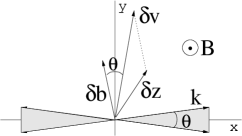
Without loss of generality we consider in detail only the structure function $S^{w}_{3L}(r)$, defined in (4), and we concentrate on the contribution provided by the configuration in which $\delta{\bf v}_{r}$ is aligned with $\delta{\bf b}_{r}$ inside a turbulent eddy. Figure 1 illustrates this case. The large-scale field ${\bf B}_{0}$ is in the z-direction and the vectors $\delta{\bf v}_{r}$ and $\delta{\bf b}_{r}$ are aligned within a small angle $\theta_{r}$ in the field-perpendicular plane, in the y-direction, say. Since the polarization of shear-Alfvén waves are perpendicular to $\mathbf{B_{0}}$ and to their wave vector $\mathbf{k}$, the wave vectors ${\bf k}$ are aligned in the x-direction here. Consequently, the variation of the fields is strongest in the x-direction and the dominant contribution to the structure function (4) comes from the situation in which the point-separation vector ${\bf r}$ lies in the x-direction. It follows from geometrical arguments that the longitudinal projection (i.e., x-component) of $\delta{\bf z}_{r}$, $\delta z_{L}$, is smaller than the typical value of $\delta w_{r}$ by a factor of order $\theta_{r}$, viz. $\delta w_{r}\sim\delta v_{r}$ and $\delta z_{L}\sim\theta_{r}\delta v_{r}$. This introduces an extra factor of $\theta_{r}$ in Politano-Pouquet correlation function (4), and one obtains

$$\langle\delta z_{L}(\delta{\bf w})^{2}\rangle\sim\theta_{r}\delta v^{3}_{r}.$$ (12)

As was demonstrated in Boldyrev (2005, 2006) and Mason et al. (2006, 2008), the scale-dependent dynamic alignment $\theta_{r}\propto r^{1/4}$ leads to the scaling of the fluctuating fields $\delta v_{r}\sim\delta b_{r}\propto r^{1/4}$, which explains the numerically observed field-perpendicular energy spectrum $E(k_{\perp})\propto k_{\perp}^{-3/2}$. Quite remarkably, by substituting these scalings into expression (12) we also satisfy the scaling relation (4). Thus, the numerical findings are reconciled with the Politano-Pouquet relations if one invokes the phenomenon of scale-dependent dynamic alignment.

Figure 1.— Sketch of the velocity and the magnetic field fluctuations, $\delta{\bf v}_{r}$ and $\delta{\bf b}_{r}$, aligned in the field-perpendicular plane within a small angle $\theta_{r}$.

In the next section we attempt to test relation (12) using numerical simulations of strong incompressible MHD turbulence. In particular, we measure the following third-order structure functions

$${\tilde{S}}_{3L}^{w}(r)=\langle|\delta z_{L}|(\delta{\bf w})^{2}\rangle,$$ (13)

$$S_{3}^{w}(r)=\langle|\delta{\bf w}|^{3}\rangle.$$ (14)

We use the absolute value of $\delta z_{L}$ in calculating (13) to avoid cancellations and slow convergence caused by different signs of $\delta z_{L}$. If our idea expressed by (12) is correct then the functions ${\tilde{S}}^{w}_{3L}(r)$ and $S_{3}(r)$ should have essentially different scalings, and, as follows from the estimate ${\tilde{S}}^{w}_{3L}(r)\sim\theta_{r}\delta v_{r}^{3}$ and $S_{3}(r)\sim\delta v_{r}^{3}$, their ratio should correspond to the alignment angle $\theta_{r}$, and therefore should scale as

$${\tilde{S}}^{w}_{3L}(r)/S^{w}_{3}(r)\propto r^{0.25}.$$ (15)

Note that the scaling of the alignment angle $\theta(r)\propto r^{0.25}$ can be measured independently with the aid of second-order structure functions (e.g., Mason et al., 2006, 2008; Beresnyak & Lazarian, 2006).

3. Numerical results

We solve the incompressible MHD equations (1, 2) using standard pseudospectral methods. An external magnetic field is applied in $z$-direction with strength $B_{0}\approx 5$ measured in units of velocity. The periodic domain has a resolution of $512^{3}$ mesh points and is elongated in the $z$-direction with aspect ratio 1:1:$B_{0}$. An external force ${\bf f}({\bf x},t)$, and small fluid viscosity $\nu$ and resistivity $\eta$ are added to the equations. The external force is random and it drives the turbulence at large scales. The details of the numerical method and set up can be found in Mason et al. (2008).

The Reynolds number is defined as $Re=U_{rms}L/\nu$, where $L$ $(\sim 1)$ is the field-perpendicular box size, $\nu$ is fluid viscosity and $U_{rms}$ $(\sim 1)$ is the rms value of velocity fluctuations. We restrict ourselves to the case in which the magnetic resistivity and fluid viscosity are the same, $\nu=\eta$, with $Re\approx 2200$. The system is evolved until a statistically steady state is reached, which is confirmed by observing the time evolution of the total energy of the fluctuations. The data set consists of 30 samples that cover approximately 6 large-scale eddy turnover times.

Figure 2.— The relative scaling of the structure functions ${\tilde{S}}^{w}_{3L}(r)$ and $S^{w}_{3}(r)$. The ratio (15) is plotted versus scale $r$. The equivalent procedure with ${\bf w}$ and ${\bf z}$ interchanged yields a similar slope. The straight line has the slope $0.2$.

To calculate the structure functions (13) and (14) we construct $\delta{\bf z}(r)={\bf z}({\bf x}+{\bf r})-{\bf z}({\bf x})$ and $\delta{\bf w}(r)={\bf w}({\bf x}+{\bf r})-{\bf w}({\bf x})$, where ${\bf r}$ is in a plane perpendicular to ${\bf B}_{0}$. By definition, $\delta z_{L}=\delta{\bf z}(r)\cdot{\bf r}/r$ and $\delta w_{L}=\delta{\bf w}(r)\cdot{\bf r}/r$. The average is taken over different positions of the point ${\bf x}$ in that plane, over all such planes in the data cube, and then over all data cubes.

The results we present here correspond to one of five simulations described in Mason et al. (2008) (Case 2a). Each of those simulations differ by the large-scale driving mechanism, which is not expected to affect the turbulent dynamics in the inertial interval. The numerical calculation of expression (15) is shown in Figure 2. For this case we find ${\tilde{S}}^{w}_{3L}(r)/S^{w}_{3}(r)\propto r^{0.2}$. Repeating the calculation for the other four cases yields noticeable scatter from case to case, with the slopes ranging from approximately $0.17$ to $0.21$. We discuss the results in the next section.

Figure 3.— Alignment regions at different scales. Plotted is $\cos(\theta)=(\mathbf{\tilde{v}}\cdot\mathbf{\tilde{b}})/|\mathbf{\tilde{v}}||\mathbf{\tilde{b}}|$ in a plane perpendicular to the guiding field $\mathbf{B_{0}}$, where $\mathbf{\tilde{v}}$ and $\mathbf{\tilde{b}}$ are the velocity and magnetic field filtered at the scale $k_{f}$. Left–right: $k_{f}=1,4,10$.

4. Discussion and conclusion

We have proposed phenomenological arguments demonstrating that the energy spectrum $E(k_{\perp})\propto k_{\perp}^{-3/2}$ for MHD turbulence is consistent with the exact analytic results that are known as the Politano-Pouquet relations. We argue that the two results are reconciled by the phenomenon of scale-dependent dynamic alignment. As a numerical illustration, we computed the structure functions (13) and (14). We found that their scalings are essentially different, which supports our arguments presented in section 2. However, the agreement with the analytic prediction ${\tilde{S}}^{w}_{3L}(r)/S^{w}_{3}(r)\propto r^{0.25}$ turns out to be only qualitative. Several reasons may explain the lack of good quantitative agreement. First, this may be due to extremely slow convergence of the statistics for the third-order structure functions in (15). Indeed we noticed that in each run the convergence of the statistics for the measured third-order structure functions is quite slow. The evolution of the slopes from snapshot to snapshot apparently has long-time variations. In spite of the large statistical ensemble accumulated in our runs, it is not enough for the precise measurement of the slope in (15). Second, the size of the Reynolds number in our simulations (which is limited by computational costs) may significantly impede computation of the slope. Third, there may be a systematic deviation of the slope measured in (15) due to intermittency corrections to the third-order structure function (14), which are not captured by our model. We plan to address these issues in future numerical work.

Finally, in Figure 3 we illustrate the regions of alignment at different scales. It appears that majority of the domain is covered with regions of high positive or negative alignment, and that this structure is hierarchical – within a large-scale region of positive alignment, say, there exist smaller scale highly aligned and anti-aligned structures. This supports our assumption that even overall balanced MHD turbulence is imbalanced locally, so that different spatial regions are responsible for different structure functions in the Politano-Pouquet relations. We note that the presence of correlated polarized regions in MHD turbulence was also observed in some early simulations (e.g., Maron & Goldreich, 2001).

References

- Beresnyak & Lazarian (2006) Beresnyak, A., & Lazarian, A. 2006, ApJ, 640, L175
- Biskamp (2003) Biskamp, D. 2003, Magnetohydrodynamic Turbulence (Cambridge University Press, Cambridge)
- Boldyrev (2005) Boldyrev, S. 2005, ApJ, 626, L37
- Boldyrev (2006) Boldyrev, S. 2006, Phys. Rev. Lett., 96, 115002
- Chandran & Cowley (1998) Chandran, B.D.G., & Cowley, S.C. 1998, Phys. Rev. Lett., 80, 3077
- Dobrowolny et al. (1980) Dobrowolny, M., Mangeney, A., & Veltri, P. 1980, Phys. Rev. Lett., 45, 144
- Frisch (1995) Frisch, U. 1995, Turbulence (Cambridge University Press, Cambridge)
- Goldreich & Sridhar (1995) Goldreich, P., & Sridhar, S. 1995, ApJ, 438, 763
- Goldstein et al. (1995) Goldstein, D. A., Roberts, D. A., & Matthaeus, W. H. 1995, ARA&A, 33, 283
- Grappin et al. (1982) Grappin, R., Frisch, U., Léorat, J., & Pouquet, A. 1982, A&A, 105, 6
- Higdon (1984) Higdon, J.C. 1984, ApJ, 285, 109
- Kulsrud & Pearce (1969) Kulsrud, R. M., & Pearce, W. P. 1969, ApJ, 156, 445
- Lithwick & Goldreich (2001) Lithwick, Y., & Goldreich, P. 2001, ApJ, 562, 279
- MacBride et al. (2008) MacBride, R. T., Smith, C. W., & Forman, M. A. 2008, ApJ, 679, 1644
- Marino et al. (2008) Marino, R., Sorriso-Valvo, L., Carbone, V., Noullez, A., Bruno, R., & Bavassano, B. 2008, ApJ, 677, L71
- Maron & Goldreich (2001) Maron, J., & Goldreich, P. 2001, ApJ, 554, 1175
- Mason et al. (2006) Mason, J., Cattaneo, F., & Boldyrev, S. 2006, Phys. Rev. Lett., 97, 255002
- Mason et al. (2008) Mason, J., Cattaneo, F., & Boldyrev, S. 2008, Phys. Rev. E, 77, 036403
- Matthaeus et al. (1996) Matthaeus, W. H., Ghosh, S., Oughton, S., & Roberts, D. A. 1996 J. Geophys. Res., 101, 7619
- Milano et al. (2001) Milano, L. J., Matthaeus, W. H., Dmitruk, P., & Montgomery, D. C. 2001, Phys. Plasmas, 8, 2673
- Müller et al. (2003) Müller, W.-C., Biskamp, D., & Grappin, R. 2003, Phys. Rev. E, 67, 066302
- Müller & Grappin (2005) Müller, W.-C., & Grappin, R. 2005, Phys. Rev. Lett., 95, 114502
- Narayan & Medvedev (2001) Narayan, R., & Medvedev, M. 2001, ApJ, 562, L129
- Perez & Boldyrev (2008) Perez, J. C., & Boldyrev, S. 2008, ApJ, 672, L61
- Perez & Boldyrev (2009) Perez, J. C., & Boldyrev, S. 2009, Phys. Rev. Lett., 102, 025003
- Podesta et al. (2009) Podesta, J.J., Forman, M.A., Smith, C.W., Elton, D.C., Malécot, Y., & Gagne, Y. 2009, preprint (arXiv:0901.3499)
- Politano & Pouquet (1998a) Politano, H., & Pouquet, A. 1998a, Geophys. Res. Lett., 25, 273
- Politano & Pouquet (1998b) Politano, H., & Pouquet, A. 1998b, Phys. Rev. E, 57, R21
- Politano et al. (1989) Politano, H., Pouquet, A., & Sulem, P. L. 1989, Phys. Fluids B, 1, 2330
- Pouquet et al. (1986) Pouquet, A., Meneguzzi, M., & Frisch, U. 1986, Phys. Rev. A, 33, 4266
- Pouquet et al. (1988) Pouquet, A., Sulem, P. L., & Meneguzzi, M. 1988, Phys. Fluids, 31, 2635
- Rechester & Rosenbluth (1978) Rechester, A. B., & Rosenbluth, M. N. 1978, Phys. Rev. Lett., 40, 38
- Vasquez et al. (2007) Vasquez, B. J., Smith, C. W., Hamilton, K., MacBride, B. T., & Leamon, R. J. 2007, J. Geophys. Res., 112, A07101
- Verma (2004) Verma, M. K. 2004, Phys. Rep., 401, 229
- Wentzel (1974) Wentzel, D. G. 1974, ARA&A, 12, 71