The Type Ia Supernova Rate at z $\approx$ 0.5 from the Supernova Legacy Survey

Abstract

We present a measurement of the distant Type Ia supernova rate derived from the first two years of the Canada – France – Hawaii Telescope Supernova Legacy Survey. We observed four one-square degree fields with a typical temporal frequency of $\langle\Delta t\rangle\sim 4$ observer-frame days over time spans of from 158 to 211 days per season for each field, with breaks during full moon. We used 8-10 meter-class telescopes for spectroscopic followup to confirm our candidates and determine their redshifts. Our starting sample consists of 73 spectroscopically verified Type Ia supernovae in the redshift range $0.2<z<0.6$. We derive a volumetric SN Ia rate of $r_{V}(\langle z\rangle=0.47)=0.42^{+0.13}_{-0.09}$ (systematic) $\pm 0.06$ (statistical) $\times 10^{-4}$ yr^-1 Mpc³, assuming $h=0.7,\Omega_{m}=0.3$ and a flat cosmology. Using recently published galaxy luminosity functions derived in our redshift range, we derive a SN Ia rate per unit luminosity of $r_{L}(\langle z\rangle=0.47)=0.154^{+0.048}_{-0.033}$ (systematic) ${}^{+0.039}_{-0.031}$ (statistical) SNu. Using our rate alone, we place an upper limit on the component of SN Ia production that tracks the cosmic star formation history of 1 SN Ia per 10³ M_⊙ of stars formed. Our rate and other rates from surveys using spectroscopic sample confirmation display only a modest evolution out to $z=0.55$.

1 Introduction

Type Ia supernovae (SNe Ia) have achieved enormous importance as cosmological distance indicators and have provided the first direct evidence for the dark energy that is driving the Universe’s accelerated expansion (Riess et al., 1998; Perlmutter et al., 1999). In spite of this importance, the physics that makes them such useful cosmological probes is only partly constrained. White dwarf physics is the best candidate for producing a standard explosion due to the well understood Chandrasekhar mass limit (Chandrasekhar, 1931). However, any plausible SN Ia scenario requires a companion to donate mass and push a sub-Chandrasekhar C-O white dwarf towards this limit producing some form of explosion (for a review, see Livio, 2001). The range of possible companion scenarios needed to accomplish this are currently divided into two broad categories: the single degenerate scenario, where the companion is a subgiant or giant star that is donating matter through winds or Roche lobe overflow (Whelan & Iben, 1973; Nomoto, 1982; Canal et al., 1996; Han & Podsiadlowski, 2004), and the double degenerate scenario involving the coalescence of two white dwarf stars after losing orbital angular momentum through gravitational radiation (Webbink, 1984; Iben & Tutukov, 1984; Tornambe & Matteucci, 1986; Napiwotzki et al., 2004).

Population synthesis models for these scenarios predict different SN Ia production timescales relative to input star formation (e.g. Greggio, 2005). By comparing the global rate of occurrence of SN Ia at different redshifts to measurements of the global cosmic star formation history (SFH), the ‘delay function’, parameterized by its characteristic timescale, $\tau$, can be derived, which in turn constrains the companion scenarios. This comparison requires the calculation of a volumetric SN Ia rate and measuring the evolution of this rate with redshift.

Early SN surveys were host targeted (e.g., Zwicky, 1938), and produced rates per unit blue luminosity that required conversion to volumetric rates through galaxy luminosity functions. These surveys suffer from large systematic uncertainties because of the natural tendency to sample the brighter end of the host luminosity function. With the advent of wide-field imagers on moderately large telescopes, recent surveys have been able to target specific volumes of space and directly calculate the volumetric rate. Examples of volumetric SN Ia rate calculations at a variety of redshifts can be found in the following studies (plotted in Figure 1): Cappellaro et al. (1999); Hardin et al. (2000); Pain et al. (2002); Madgwick et al. (2003); Tonry et al. (2003); Blanc et al. (2004); Dahlen et al. (2004); Barris & Tonry (2006).

We plot the rates from these surveys as a function of redshift in Figure 1, along with a recent SFH fit from Hopkins & Beacom (2006), renormalized by a factor of $10^{3}$. This allows us to compare the SFH to the observed trend in the SN Ia rate. This trend, compared with the SFH curve, shows some curious properties. The large gradient just beyond $z=0.5$ observed in Barris & Tonry (2006) has no analog in the SFH curve, and neither does the apparent down-turn beyond $z=1.2$ observed by Dahlen et al. (2004). Fits of the delay function to various subsets of these data have produced no consensus on $\tau$, or the form of the delay. Reported values for $\tau$ range from as short as $\tau\leq$ 1 Gyr (Barris & Tonry, 2006) to as long as $\tau=2-4$ Gyr (Strolger et al., 2004). This lack of consensus and the peculiar features in Figure 1 argue that systematics are playing a role in the observed SN Ia rates, especially at higher redshifts. It is vital to investigate the sources of systematic error in deriving SN Ia rates and to compare the cosmic SFH with rates that have well characterized systematic errors.

In this paper we take advantage of the high-quality spectroscopy and well-defined survey properties of the Supernova Legacy Survey (SNLS, Astier et al., 2006) to produce a rate that minimizes systematics, which we then compare with cosmic SFH. To minimize contamination, we use only spectroscopically verified SNe Ia in our sample. We examine sources of systematic error in detail and, using Monte Carlo efficiency experiments, place limits on them. In particular, we improve upon previous surveys in the treatment of host extinction by using the recent dust models of Riello & Patat (2005). We also investigate the possibility that SNe Ia are being missed in the cores of galaxies with fake SN experiments using real SNLS images. These experiments allow us to place limits on our own errors and assess the impact of various sources of systematic error on SN surveys in general.

In order to avoid large and uncertain completeness corrections, we employ a simplification in our rate determination that fully exploits the data set currently available: we restrict our sample to the redshift range $0.2<z<0.6$. This ensures that the majority of SNe Ia peak above our nominal detection limits and thus provides a high completeness. This simplification allows us to extract a well-defined sample of spectroscopically verified SNe Ia from the survey and accurately simulate the SNLS survey efficiency, thus producing the most accurate SN Ia rate at any redshift. Our rate alone is sufficient to constrain some of the SFH delay function models by placing limits on their parameters.

The structure of the paper is as follows. In §2 we describe the survey properties relevant to rate calculation. In §3 we develop objective selection criteria, derive our SN Ia sample and analyze this sample to determine our spectroscopic completeness. In §4 we describe our method for calculating the survey efficiency and present the results of these calculations. In §5 we present the derived SN Ia rates per unit volume and per unit luminosity, an analysis of systematic errors, and a comparison of our rates with rates in the literature. In §6 we compare our volumetric rate and a selection of rates from the literature with two recent models connecting SFH with SN Ia production.

For ease of comparison with other rates studies in the literature, we assume a flat cosmology throughout with $H_{0}=70$ km s^-1 Mpc^-1, $\Omega_{\Lambda}=0.7$, and $\Omega_{M}=0.3$.

2 The Supernova Legacy Survey

The SNLS is a second-generation SN Ia survey spanning five years, instigated with the purpose of measuring the accelerated expansion of the universe and constraining the average pressure-density ratio of the universe, $\langle w\rangle$, to better than $\pm 0.05$ (Astier et al., 2006). In order to achieve this goal, the SNe Ia plotted on our Hubble diagram must have well-sampled light curves (LCs) and spectral followup observations that provide accurate redshifts and solid identifications. The LC sampling is achieved using MegaCam (Boulade et al., 2003), a 36 CCD mosaic one-square degree imager, in queued service observing mode on the 3.6 meter Canada-France-Hawaii Telescope (CFHT). This combination images four one-square degree fields (D1-4, evenly spaced in right ascension, see Table 1) in four filters ($g^{\prime}$$r^{\prime}$$i^{\prime}$$z^{\prime}$) with an observer-frame cadence of $\Delta t\sim 4$ days (rest-frame cadence for a typical SN of $\Delta t\sim 3$ days) and with a typical limiting magnitude of 24.5 in $i^{\prime}$. The queued service mode provides robust protection against bad weather, as any night lost is re-queued for the following night.

This observing strategy provides dense LC coverage for SNe Ia out to $z\sim 1$ and is ideal for measuring the rate of occurrence of distant SNe Ia. It also produces high quality SN Ia candidates identified early enough so that spectroscopic followup observations can be scheduled near the candidate’s maximum light (Sullivan et al., 2006). This strategy has been very successful (Howell et al., 2005), and the SNLS has been fortunate to have consistent access to 8-10 meter class telescopes (Gemini, Keck, VLT) for spectroscopic followup. This is critical for providing a high spectroscopic completeness and the solid spectroscopic type confirmation required to remove contaminating non-SN Ia objects from our sample (Howell et al., 2005; Basa et al., 2006).

2.1 The Detection Pipeline

The imaging data are analyzed by two independent search pipelines in Canada and France. For the rate calculation in this paper, we use the properties of the Canadian pipeline.

The Canadian SNLS real-time pipeline uses the $i^{\prime}$ filter images for detection of SN candidates and images in all filters for object classification. Each epoch consists of five to ten exposures which undergo a preliminary (real-time) reduction which includes a photometric and astrometric calibration before being combined. A reference image for each field is constructed from previously acquired, hand picked, high-quality images. The detection pipeline then seeing-matches the reference image to the (usually lower image quality) new epoch image (Pritchet et al., 2006). The seeing-matched reference image is then subtracted from the new epoch and the resulting difference image is analyzed to detect variable objects which appear as residual (positive) point sources. A final list of candidate variable objects is produced from this difference image in two stages: first, a preliminary candidate list is generated using an automated detection routine and then, a final candidate list is culled by human review of the preliminary list. This visual inspection is conducted by one of us (D.B.) and is essential for weeding out the large quantity of non-variable objects (image defects, and PSF matching errors) that remain after the automated detection stage.

At this stage, all candidate variables are given a preliminary classification and any object that may possibly be a SN (of any type) has ‘SN’ in its classification. The new measurements of variable candidates are entered into our object database and compared with previously discovered variable objects. This comparison weeds out previously discovered non-SN variables such as AGN and variable stars from the SN candidate list. All measurements of the current SN candidates, including recent non-detections, are then evaluated for spectroscopic followup using photometric selection criteria.

The details of the photometric selection process for the SNLS are presented in Sullivan et al. (2006). In brief, all photometric observations of the early part of the LC of a SN candidate are fit to template SN Ia LCs using a $\chi^{2}$ minimization in a multi-parameter space that includes redshift, stretch, time of maximum light, host extinction, and peak dispersion. The template LCs are generated from an updated version of the SN Ia spectral templates presented in Nugent et al. (2002). These spectral templates are multiplied by the MegaCam filter response functions and integrated, thus accounting for k-corrections (Sullivan et al., 2006). The results of this fit are used to measure a photometric redshift, $z_{PHOT}$, for the candidate and to make a more accurate classification. If there is any doubt about the nature of the object, the ‘SN’ classification is retained in the database.

All SN candidates in the database are available for the observers doing spectroscopic followup. The quality of the candidate, deduced from the template fit and an assessment of usefulness for cosmology, is used to prioritize the candidates for spectroscopic observation. Once these observations are taken, they are reduced and compared to SN Ia spectral templates (Howell et al., 2005; Basa et al., 2006) to calculate a spectroscopic redshift, $z_{SPEC}$. The final typing assessment uses all available information, both photometric and spectroscopic. The photometry provides early epoch colors, which can help identify CC SNe. It also provides an accurate phase for the spectroscopic observation which is also important in discriminating SNe Ia from CC SNe. The galaxy-subtracted candidate spectrum is then checked for the presence of spectral features peculiar to SNe Ia. We then assign a likelihood statistic for the candidate’s membership in the SN Ia type (Howell et al., 2005).

3 Selection Criteria

Selection criteria are used to provide consistency between the observed sample, the survey efficiency calculation, and the completeness calculation and thus produce an accurate rate. In practice, they serve to objectify the survey goals and properties (which unavoidably include the human element) such that efficiency simulations are accurate and tractable. The criteria we developed consist of the minimum required photometric observations, expressed in terms of rest-frame epoch and filter, that guarantee that any real SN Ia acquires spectroscopic followup. They were derived by examining the photometric observations of all our spectroscopically confirmed SNe Ia in the redshift range $0.2<z<0.6$. To account for any real SN Ia that meet these criteria but, for one reason or another, did not acquire spectroscopic followup, we also apply these criteria to our entire ’SN’ candidate list in a completeness study (see below).

Since the primary goal of the SNLS is cosmology, when selecting SN candidates for spectroscopic followup we attempt to eliminate objects, even SNe Ia, that offer no information for cosmological fitting. Examples of these include SNe for which no maximum brightness can be determined, or for which no stretch or no color information can be measured. Thus, the objective criteria that define our sample and survey efficiencies are expressed by requiring each confirmed SN Ia to have the following observations:

1. one $i^{\prime}$ detection at $S/N>10.0$ between restframe day -15.0 and day -1.5

2. two $i^{\prime}$ observations between restframe day -15.0 and day -1.5

3. one $r^{\prime}$ observation between restframe day -15.0 and day -1.5

4. one $g^{\prime}$ observation between restframe day -15.0 and day +5.0

5. one $i^{\prime}$ or $r^{\prime}$ observation between restframe day +11.5 and +30.0

Criterion 1 and 2 implement our need to detect candidate SNe Ia early enough to schedule spectroscopic observations near maximum brightness. Criterion 2 is required to judge if the LC is rising or declining. Criteria 3 and 4 are required because an early color is important for photometrically classifying the SN type. Criterion 5 implements the requirement that stretch information be available for any cosmologically useful SN Ia. We only require the detection in the pre-max $i^{\prime}$ because during the early part of the light curve SNe Ia are distinguished from other SN types by having redder colors. Thus, if we have an early detection of a candidate in $i^{\prime}$, but can only place a limit on the object in $r^{\prime}$ or $g^{\prime}$, then it would have a reasonably high probability of being a SN Ia and is likely to be spectroscopically followed up. This also means that highly reddened SNe are not selected against. For this redshift range, we need not be concerned with criteria based on the $z^{\prime}$ filter. Criterion 5 would not logically enter the selection process as a detection, since these observations could not be taken before the decision to followup is made. It is included solely to remove objects that are discovered close to the end of an observing season, when there is no hope of obtaining the observations needed to derive a stretch value.

It is important to point out that these criteria are independent of the LC fitting that is normally done in candidate selection, i.e., there are no criteria involving the SN Ia fit $\chi^{2}$. This is because we defined these criteria with spectroscopically confirmed SNe Ia. The fitting is required to derive the type and the redshift of candidate SNe. In our sample selection both of these quantities are given by the spectroscopy. In the efficiency simulations, we are only interested in our detection efficiency for SNe Ia, so the type is defined a priori, and the redshifts are given by the Monte Carlo simulation (see below). The LC fitting does enter into the completeness study, since we are then interested in objects without spectroscopy. We describe the LC fitting criteria used to derive an accurate completeness, given the above selection criteria, in §3.2.

3.1 The Observed Sample

In order to define an observed sample consistent with these survey selection criteria, we must eliminate spectroscopically confirmed SNe Ia in the initial list that do not meet these criteria. These ‘special-case’ SNe Ia acquired spectroscopic followup for two reasons. First, during some of our initial runs we attempted to spectrally follow up nearly every suspected SN to help refine our photometric selection criteria. Second, occasionally bad weather can prematurely end a field’s observing season before all the good declining candidates have the required observations to determine their stretch values.

We derived our starting SN Ia sample from all spectroscopically confirmed SNe Ia with a spectroscopic redshift, $z_{SPEC}$, in the range $0.2<z_{SPEC}<0.6$, discovered in the first two full seasons of each deep field. The starting and ending dates and resulting time span in days is listed for each season of each field in Table 1. Figure 15 illustrates the field observing seasons for the sample by plotting the Julian Day of the epochs versus their calculated limiting $i^{\prime}$ magnitude (see §4.1).

Table 2 individually lists the 73 spectroscopically confirmed SNe Ia from the SNLS that comprise our starting sample. Column 1 gives the SNLS designation for the SN, columns 2 and 3 give the J2000.0 coordinates, column 4 gives the redshift, column 5 gives the MJD of discovery, column 6 indicates if the object was culled from the initial list by enumerating which of the criteria from §3 it failed, and column 7 lists the references in which further information about the object is published. The table is ordered by field and by time within each field with breaks between the two seasons of the given field.

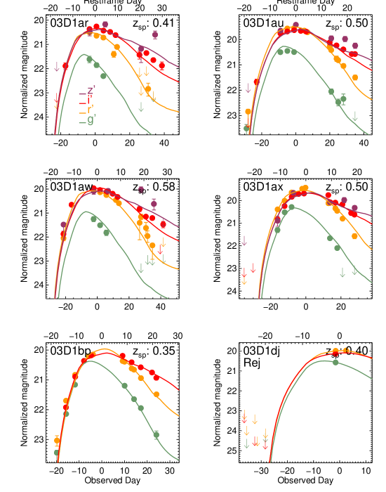
Figure 2: Nighly averaged photometry for the spectroscopically confirmed sample of SNLS SNe Ia. Each filled circle represents the nightly average magnitude for the $g^{\prime}$ (green), $r^{\prime}$ (orange), $i^{\prime}$ (red), and $z^{\prime}$ (purple) filters on a normalized AB magnitude scale. The template fits for each filter are indicated by the solid lines of the corresponding color. The designation from Table 2 (minus the SNLS prefix) is indicated in the upper left corner and the spectroscopic redshift is indicated in the upper right corner of each panel. If the SN was culled from the sample, this is indicated by the word ‘Rej’ under the designation. The remaining SNe are presented in the following pages.

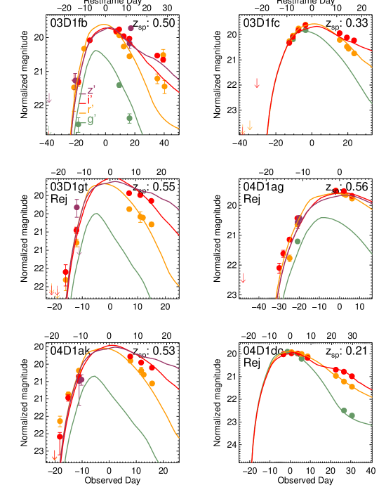
Figure 2: continued.

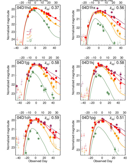
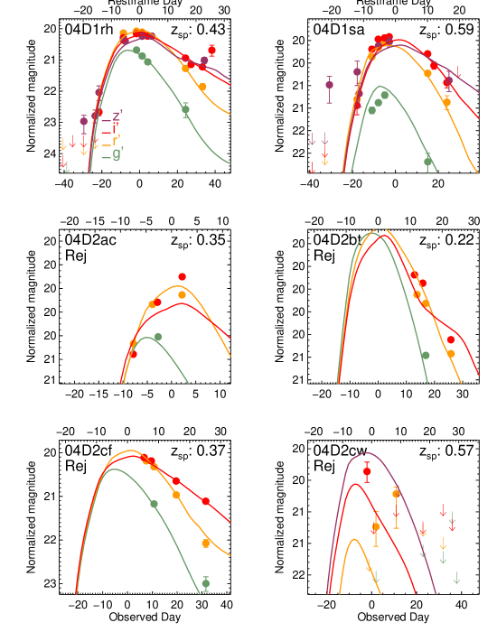
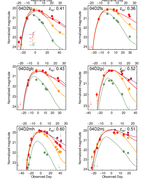
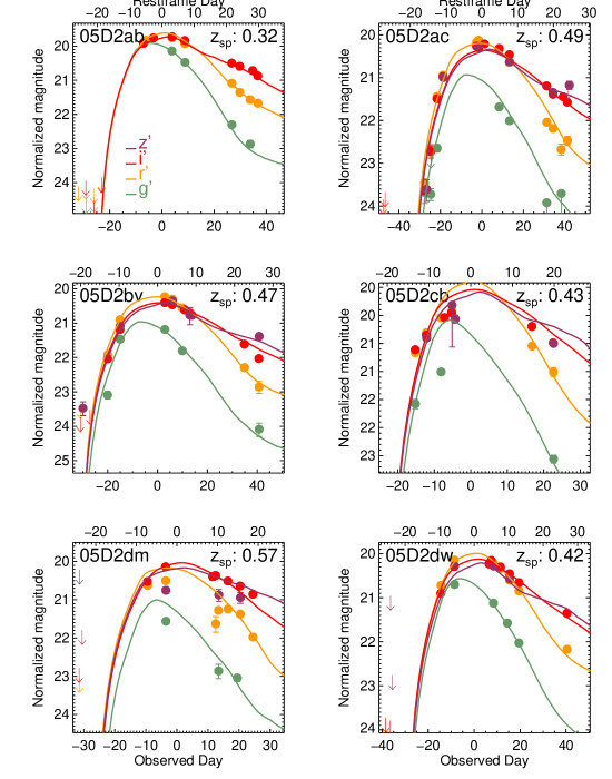
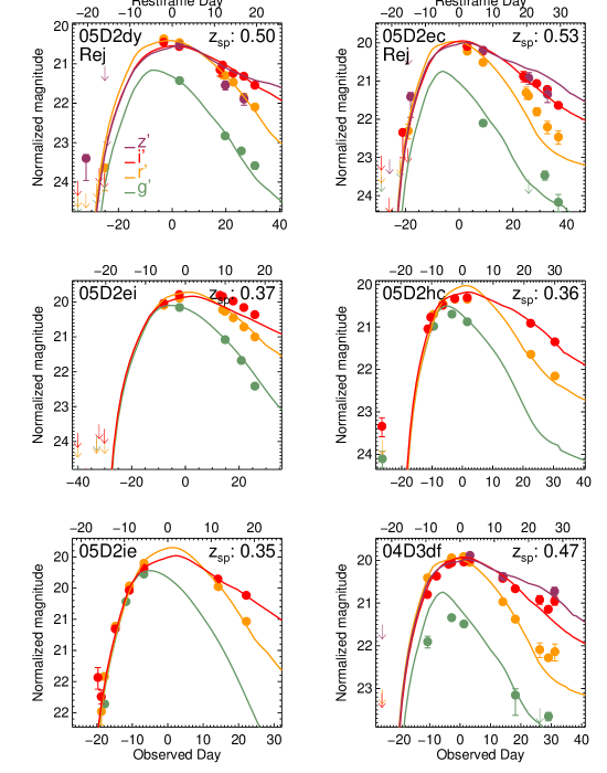
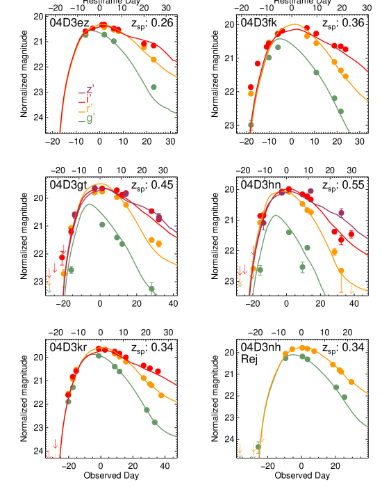
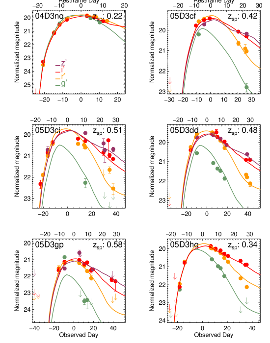
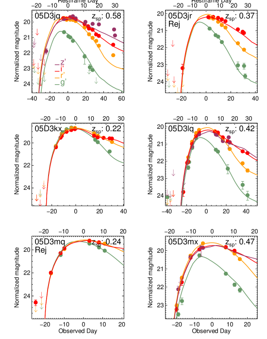
Figure 2: continued.

Figure 2: continued.

Figure 2: continued.

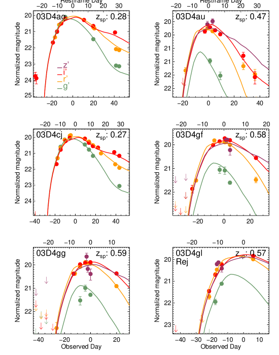
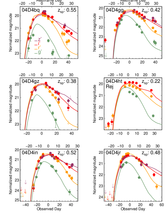
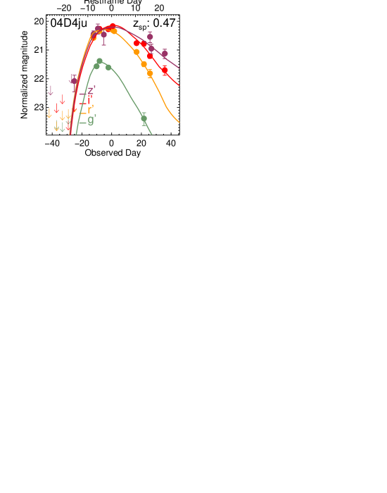
Figure 2: continued.

Figure 2 plots the nightly averaged photometry for each of the 73 spectroscopically confirmed SNe Ia from Table 2 with 1$\sigma$ error bars on a normalized AB magnitude scale. The best-fit SN Ia template is overplotted (Sullivan et al., 2006). The magnitude scale is normalized such that the brightest tick mark is always 20 magnitudes. This procedure preserves the relative magnitude difference between filters for a given SN. The day scale on the bottom of each plot is the observed day relative to maximum light. The day scale on the top is the restframe day relative to maximum light. The designation from Table 2 (minus the SNLS prefix) is given in the upper left corner and the spectroscopic redshift in the upper right corner of each panel. If the object was culled from the initial list, this is indicated under the designation with the word ‘Rej’ (e.g. SNLS-03D1dj was culled).

Almost every object from season one of each field is included in the cosmology fit of Astier et al. (2006). The three exceptions are SNLS-03D1ar, which had insufficient observations at the time, SNLS-03D4cj, which was a SN 1991T-like SN Ia, and SNLS-03D4au, which was under-luminous, most likely due to extinction. We point out that even though these objects were excluded from the cosmology fit, their identity as SNe Ia has never been in doubt. The objects that were observed with Gemini have their spectra published in Howell et al. (2005). The objects observed with the VLT will have their spectra published shortly in Basa et al. (2006). The remaining 10 objects from the first seasons were observed with Keck.

The sample is summarized in Table 3, which lists, for each season of each field, the total number of spectroscopically confirmed SNe Ia and the number after culling the starting list using our objective selection criteria.

3.2 Spectroscopic Completeness

We now calculate the number of objects that passed our selection criteria but, for one reason or another, were not spectrally followed up. This calculation is aided by the high detection completeness of the survey below $z=0.6$ (see §4.2.3), and the classification scheme we use, where any object remotely consistent with a SN LC, after checking for long-term variability, retains the ‘SN’ in the classification. We are also able to use a final version of the photometry, generated for all objects in our database from images that have been de-trended with the final calibration images for each observing run. This final photometry, which now covers all phases of the candidate LCs, is fit with SN Ia templates as described above to produce a more accurate $z_{PHOT}$ and a $\chi^{2}_{SNIa}$ for the $\chi^{2}$ of the SN Ia template fit to the photometry in all filters. We examined all objects with a final photometry $z_{PHOT}$ in the range $0.2<z_{PHOT}<0.6$ discovered within the time spans in Table 1 with the following classifications: ‘SN’, ‘SN?’, ‘SNI’, ‘SNII’, ‘SNII?’, ‘SN/AGN’, and ‘SN/var?’. We measured the offset and uncertainty in our $z_{PHOT}$ fitting technique by comparing $z_{PHOT}$ with $z_{SPEC}$ and found a mean offset of $\Delta z<10^{-3}$ and an RMS scatter of $\sigma_{z}=0.08$. We, therefore, assume that the remaining error in $z_{PHOT}$ from the the final photometry is small and random such that as many candidates are scattered out of our redshift range of interest as are scattered in.

Of 180 objects from the sample time ranges with ‘SN’ in their type, 50 do not have the required observations from our object selection criteria listed above and so, even if they were SNe Ia, would not be included in our culled sample. Of the remaining 130 objects, 64 are rejected because their fit to the templates has a $\chi^{2}_{SNIa}>10.0$ and so very unlikely to be SNe Ia (Sullivan et al., 2006). We then apply an upper limit stretch cut, requiring $s<1.35$, to the remaining 66 objects. Objects with $s>1.35$ are also not SNe Ia (see Astier et al. 2005, Figure 7 and Sullivan et al. 2006b, Figure 3). These objects are probably SNe IIP which have a long plateau in their LCs and hence produce anomalously high $s$ values when fit with a SN Ia template. The $s<1.35$ cut removes 33 objects. We then make a cut by examining the early colors and remove those that have large residuals in this part of the LC as a result of being too blue (one signature of a core-collapse SN). Of the remaining 33 objects, 14 of these are rejected as too blue in the early colors, even though the overall $\chi^{2}_{SNIa}$ is less than 10.0. We are left with 19 unconfirmed SN Ia candidates that have a reasonable probability of being missed, real SNe Ia.

Table 4 lists the 19 unconfirmed SN Ia candidates, their coordinates, their $z_{PHOT}$, discovery date, initial type, $\chi^{2}_{SNIa}$, and their status. We group them into those with $\chi^{2}_{SNIa}<5.0$ and those with $\chi^{2}_{SNIa}>5.0$ and consider those in the first group to be probable SNe Ia, and those in the second group to be possible SNe Ia. We point out that the intrinsic variation in SN Ia LCs rarely allow template fits with $\chi^{2}_{SNIa}<2$, and that typical fits have $\chi^{2}_{SNIa}$ in the range 2-3 (Sullivan et al., 2006). We take the conservative approach that, aside from the division at $\chi^{2}_{SNIa}=5.0$, we must consider each candidate in each group as equal. This then determines the range of completeness we consider in calculating our systematic errors (see below). Our most likely completeness is defined by assuming that each ‘Probable SN Ia’ in this list is, in fact, a real SN Ia and each ‘Possible SN Ia’ is not. The minimum completeness is defined by the scenario that all 19 are real SN Ia and the maximum completeness is defined by the scenario that none of the 19 are real, which amounts to 100% completeness. We tabulate the confirmed, probable and possible SNe Ia and the minimum and most likely completeness for each field and the ensemble in Table 5. We will use this table when we compute our systematic errors in §5.3.1.

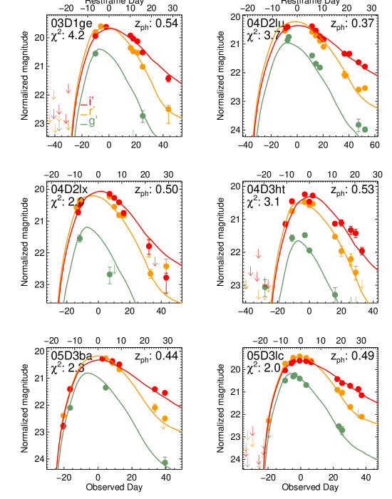
Figure 16: Nighly averaged photometry (as in Figure 2) for the unconfirmed SNLS SNe Ia from Table 4. The designation is in the upper left corner and the photometric redshift is in the upper right corner of each panel. The $\chi_{SNIa}^{2}$ values from Table 4 are printed under the designation for each SN. The first six objects are presented here. The full set is available from the online version of the article.

Figure 16 plots the nightly average photometry for the 19 unconfirmed SN Ia candidates from Table 4 using the same normalized AB magnitude scale and day axes as in Figure 2. The photometric redshift is indicated in the upper right corner of each panel. The $\chi^{2}_{SNIa}$ value from Table 4 for each SN is indicated under its designation on each panel.

4 Survey Efficiency

Since Fritz Zwicky’s pioneering efforts to estimate supernova rates from photographic surveys using the control-time method (Zwicky, 1938), there have been significant improvements in calculating a given survey’s efficiency (for a review see Wood-Vasey, 2005, Chapter 6). As a recent example, Pain et al. (1996) used SN Ia template LCs to place simulated SNe in CCD survey images to generate a Monte Carlo simulation that produced a much more accurate efficiency for their survey. Most recent surveys using CCDs have performed some variation of this method to calculate their efficiencies and from them derive their rates (Hardin et al., 2000; Pain et al., 2002; Madgwick et al., 2003; Blanc et al., 2004).

In our particular variation on this method, we do not place artificial SNe on every image of our survey. Instead, we characterize how our frame limits vary with relevant parameters (such a seeing) using a subset of real survey images. We then use this characterization to observe a Monte Carlo simulation which uses the updated SN Ia spectral templates of Nugent et al. (2002) and our survey filter response functions to generate the LCs from a large population of realistic SNe Ia. Thus, to calculate an appropriate survey efficiency, we need to implement the objective selection criteria defined above in a Monte Carlo efficiency experiment that simulates the observation of the SN Ia LCs by the SNLS. Criteria 2-5 (see §3) can be implemented simply by inputting the date and filter of each image in the survey sample time ranges, and seeing if we have the required observations for each simulated candidate. Criterion 1 specifies a detection in the $i^{\prime}$ filter, which requires that we calculate the SN visibility at each $i^{\prime}$ epoch in the survey sample time ranges.

4.1 $i^{\prime}$ SN Visibility

The photometric depth reached by a given $i^{\prime}$ observation depends on the exposure time ($E_{e}$), image quality ($IQ_{e}$), airmass ($X_{e}$), transparency ($T_{e}$), and the noise in the sky background ($S_{e}$). Some of these data are trivially available from each image header. The transparency and the sky background must be derived from the images themselves.

Our final photometry pipeline includes a photometric calibration process that calculates a flux scaling parameter, $F_{e}$, for each image. We calculate it by comparing a large number of isolated sources in the object image with the same objects in a (photometric) reference image. The resulting $F_{e}$ values are applied to each object image to ensure that the flux measured for a non-variable object is the same in each epoch. Thus, $F_{e}$ accounts for variations in both $T_{e}$ and $X_{e}$. An image with lower transparency and/or higher airmass will have a larger $F_{e}$. During this process the standard deviation per pixel in the sky is also calculated, allowing us to account for variations in $S_{e}$. The total number of usable CCD chips, out of the nominal 36, is also tabulated (see §4.1.2).

Another factor that determines a spatially localized frame limit is the galaxy host background light against which the SN must be discerned ($H_{i^{\prime},gal}$). This depends on the brightness and light profile of the host and the brightness and position of the SN within the host. This dependence is mitigated somewhat by the subtraction method used in our detection pipeline (see §2.1), but must still be measured.

We designed a controlled experiment to explore the effects of $IQ_{e}$, and $H_{i^{\prime},gal}$ on SN visibility. This experiment places many artificial SNe of varying brightness and host galaxy position (yielding a range of $H_{i^{\prime},gal}$) in real SNLS detection pipeline images of varying $IQ_{e}$. We chose a range of $IQ_{e}$ from $IQ_{e}=0"\kern-4.83694pt.\kern 0.99585pt60$, close to the median for the survey, to $IQ_{e}=1"\kern-4.83694pt.\kern 0.99585pt06$, near the limit of acceptability. We used epochs with the canonical exposure time of 3641s and required that the images were taken under photometric conditions.

Prior to the addition of fake SNe, each image was analyzed with SExtractor (Bertin & Arnouts, 1996) to produce a list of potential galaxy hosts over the entire image. For a given fake SN, the host was chosen from this list using a brightness weighted probability, such that brighter galaxies are more likely to be the host than fainter galaxies. The location within the host for the fake SN was also chosen with a brightness weighted probability, such that more SNe are produced where the galaxy has more light (i.e. toward the center). Once the location within the pipeline image is decided, a nearby isolated, high S/N star was scaled to have a magnitude in the range $21.0<i^{\prime}<27.0$ and added at the chosen position.

There was no correlation of the fake SN magnitude with the host magnitude, therefore, our simulations were relevant for SNe at all phases of their LC. This spatial distribution and magnitude range allows us to quantify any systematic loss of SN visibility near the cores of galaxies in our recovery experiments (see below). Once a set of these images was produced it was put through the same detection pipeline used by the Canadian SNLS for detecting real SNe (Perrett et al., 2006; Sullivan et al., 2006; Astier et al., 2006).

Figure 20 shows the raw recovery percentage of $\sim$ 2000 fake SNe after the human review process for two $IQ_{e}$ values: $0"\kern-4.83694pt.\kern 0.99585pt69$ and $1"\kern-4.83694pt.\kern 0.99585pt06$. The 50% recovery limits are indicated and are the most useful for rate calculation since the visible SNe missed below these limits are gained back by including the invisible SNe above the limits (see Figure 20a). The loss in visibility going from automatic detection to human review amounts to a brightening of the visibility limits of only 0.1 magnitudes at the small $IQ_{e}$ value. Figure 20b shows no trend with host offset and Figure 20d shows that the cutoff due to background brightness is 20 mag arcsecond^-2. A notable feature of Figure 20a is the maximum recovery percentage of 95% for the $IQ_{e}=0"\kern-4.83694pt.\kern 0.99585pt69$ image. We examined the spatial distribution of the fake SNe from this image that were missed above $i^{\prime}=23$ to try to understand the source of this limit on the recovery. We saw no correlation with galaxy host offset, proximity to bright stars, or placement on masked or edge regions. This feature appears to be purely statistical in origin and we account for it when observing the Monte Carlo simulations (see §4.2).

Figure 21 shows the 50% recovery limits derived from the fake SN experiments using nine $i^{\prime}$ images having a range of $IQ_{e}$. These limits have been corrected for sky noise, transparency, and exposure time differences. We plot the histogram of all the $IQ_{e}$ values for all $i^{\prime}$ images relevant to this study as a dashed line. All points are derived at the automated detection stage unless otherwise indicated. The corrected results of the human review experiment from above are plotted as asterisks. We fit the human review limits with a linear fit (shown as the solid line) and this fit represents an upper bound on the limits of the images we sampled. A constant frame limit of $i^{\prime}=24.5$ is shown as the solid horizontal line and is a reasonable lower bound. The two solid lines encompass all points in Figure 21. We will use the human review limit fit as our best estimate of the frame limit versus $IQ_{e}$ function, with the constant limit as an estimate for the systematic error in our rates due to the $i^{\prime}$ frame limits (see §5.3).

4.1.1 $i^{\prime}$ SN Visibility Equation

Our fake SN experiments have provided a way to calculate the visibility limit in magnitudes, $L_{e}$, for any $i^{\prime}$ epoch in our survey sample time span using the following formula:

$$L_{e}=L_{0.5}-\alpha(IQ_{e}-0.5)+2.5\log(E_{e}/E_{ref})-2.5\log(F_{e})-2.5\log(S_{e}/S_{ref}),$$ (1)

where $L_{0.5}$ is reference visibility limit for an epoch with $IQ_{e}=0"\kern-4.83694pt.\kern 0.99585pt5$, $F_{e}=1.0$, exposure time of $E_{ref}$ seconds and sky noise of $S_{ref}$ counts, $\alpha$ is the proportionality factor between $IQ_{e}$ and the visibility limit, $E_{e}$ is the exposure time of the epoch, $F_{e}$ is the flux scale factor, and $S_{e}$ is the sky noise in counts of the epoch (see Figure 15). This formula assumes a linear relationship between $IQ_{e}$ and $L_{e}$, which appears to be a reasonable approximation over the range of $IQ_{e}$ used to discover SNe (see Figure 21).

Table 6 lists the parameters calculated using the 50% recovery fraction visibility limits determined from the human review recovery experiment (see Figure 20 and 21). Columns 1 and 2 of Table 6 lists the $IQ_{e}$ for the pair of good and bad $IQ$ images used in the human review experiment, column 3 lists the reference exposure time, column 4 lists the reference sky noise in counts, column 5 lists the visibility limit at $IQ=0"\kern-4.83694pt.\kern 0.99585pt5$, and column 6 lists the proportionality constant between $IQ_{e}$ and $L_{e}$. For the reference sky noise, $S_{ref}$, we used the value from the good $IQ$ image and adjusted the limit from the poor $IQ$ image to correspond to an image with the same sky noise as the good $IQ$ image.

4.1.2 Temporary CCD Losses

Another factor affecting the visibility of SNe in the SNLS must be accounted for. Occasionally, a very small subset of the 36 MegaCam CCDs will malfunction for a short time, usually because of a failure in the readout electronics. An even rarer occurrence is the appearance of a condensate of water on the surface of one of the correctors that covers a localized area of the field of view rendering that part of the detector temporarily useless for the detection of SNe. When we calculate the fluxscale factors mentioned above, the number of usable CCDs is also recorded. This number is used to account for these localized, temporary losses of SN visibility (see below).

4.2 Monte Carlo Simulation

The Monte Carlo technique allows us to determine our survey efficiency to a much higher precision than permitted by the small number of observed events. Using observed SN Ia LC properties and random number generators, we simulate a large ($N=10^{6}$) population of SN Ia events in the sample volume occurring over a two year period centered on the observed seasons for the field. This large number is sufficient to drive the Poisson errors down to $\sqrt{N}/N=0.1$%. This population is then observed by using real SNLS epoch properties and equation 1, combined with our objective selection criteria, to define the number of simulated spectroscopic SN Ia confirmations. This number is divided by the number of input simulated SNe Ia to derive the yearly survey efficiency.

4.2.1 Generating the Sample Population

To simulate a realistic population of Type Ia SNe, we use the same LC templates and software used to determine photometric redshifts for the SNLS candidate SNe (Sullivan et al., 2006). Figure 22 shows the canonical distributions of the parameters that characterize SN Ia LCs used in our efficiency simulations. The redshifts are chosen with a volume weighted uniform random number generator, to produce a redshift distribution over the range $0.2<z<0.6$ that is uniform per unit volume as shown in Figure 22a. We also calculated the run of $dV(z)$, given the cosmological parameters from §1, and over-plotted this as a dashed line (with an offset of $F=0.005$ for clarity) to show that our distribution is indeed constant per unit volume. The stretch values are selected using a Gaussian distribution centered on 1 with a width of $\sigma_{s}=0.1$ (Figure 22b). The intrinsic SN color is determined using the stretch-color relation from Knop et al. (2003). The host color excesses are chosen from the positive half of a Gaussian distribution, centered on 0.0 with a width of $\sigma_{E(B-V)_{h}}=0.2$ (Figure 22c). These are converted to host extinction assuming an extinction law with $R_{V}=3.1$ (Cardelli et al., 1989). The peak magnitude offsets (after stretch correction) shown in Figure 22d are chosen from a Gaussian distribution centered on 0 with a width of $\sigma_{B_{MAX}}=0.17$ (Hamuy et al., 1996). A uniform random number generator is used to pick the day of maximum for each simulated SNe Ia from a two-year-long interval that is centered on the middle of the survey range being simulated. This avoids problems with edge effects and produces an efficiency per year. We will address the systematic uncertainty due to differences between these distributions and the true distributions in §5.3.

In order to account for the possibility that a given SN can be missed because of temporary localized losses of SN detectability in the Megacam array (see above, §4.1.2), we assign a pseudo-pixel position to each simulated SN. This is done with a uniform random number generator that selects one of the 370 million Megacam pixels that are nominally available as the location of the SN. The number of real pixels available on a given epoch is calculated from the number of usable chips, derived during the fluxscale calculation. By choosing a random number out of 370 million, we are essentially assigning a probability that the SN will land on a region of the array that is temporarily unusable. If all chips are working, then the number of pixels available equals the nominal number and no SNe are lost. If a large number of chips are not working, the the number of pixels available is much less than the nominal number and a simulated SN has a higher probability of being missed.

4.2.2 Observing the Sample Population

With the input sample population defined and LCs covering the simulated period generated, we use the data describing the real SNLS survey epochs to observe the simulation. First, we use an average Milky Way extinction appropriate for the field being simulated (Astier et al., 2006, Table 1). Then we use the epoch properties, equation 1, and Table 6 to calculate visibility limits for each $i^{\prime}$ epoch. These visibility limits are used to define the signal-to-noise ratio, $S/N$, for each simulated SN observation using the following formula:

$$S/N=10.0\times 10^{[-0.4(m_{e}-L_{e})]},$$ (2)

with $m_{e}$ being the template magnitude of the simulated SN Ia in the epoch, and $L_{e}$ the epoch 50% visibility limit. This formula assumes that an observation at the 50% visibility limit has a $S/N$ of 10. The calculated $S/N$ defines the width of a Gaussian noise distribution and a Gaussian random number generator is used to pick the noise offset for the observation.

After the noise offsets are added to the observations, the resulting magnitudes in each epoch are then compared with the corresponding $i^{\prime}$ visibility limits, $L_{e}$, and any magnitude that is brighter than its corresponding limit is considered an $i^{\prime}$ detection. We use a uniform random number generator to assign a real number ranging from 0.0 to 1.0 for each $i^{\prime}$epoch. If this number exceeds 0.95, then the candidate is not detected in that epoch. This accounts for the 95% maximum recovery fraction observed in Figure 20a. The shape of the recovery fraction at fainter magnitudes is already accounted for by using the 50% recovery magnitudes in the visibility limit calculation (see Figure 20a). To account for localized visibility losses, we calculate the number of pixels available on the epoch from the number of good CCDs available on that epoch. If the candidate was assigned a pseudo-pixel number larger than the number of good pixels on the epoch, then the candidate is not detected on that epoch.

The restframe phases (relative to peak brightness) of all the relevant $i^{\prime}$ epochs are calculated for each simulated SN Ia using its given redshift. If a simulated SN Ia ends up with a detection in the restframe phase range from criterion 1 (see §3) then we evaluate it with respect to the remaining criteria. We calculate the restframe phase for each observation in the $g^{\prime}$, and $r^{\prime}$ epochs and then the remaining criteria are applied to decide if the simulated SN should be counted as a spectroscopically confirmed SN Ia.

For the yearly efficiency, we keep track of the total number of SNe Ia that are simulated, since they are generated in yearly intervals. We also keep track of the number of SNe Ia that were simulated during the observing season for each field (from 158 to 211 days, see Table 1). This allows us to compute our on-field detection efficiency and our on-field spectroscopic confirmation efficiency.

4.2.3 The Monte Carlo Survey Efficiency

The resulting efficiencies for each field are presented in Table 7. As we stated above, the statistical errors in these numbers are $\sim$0.1%. We present the on-field $i^{\prime}$ detection efficiencies in column 2, which are all within 5% of 100%. This is expected considering the redshift range of our sample and the nominal $i^{\prime}$ frame limits. It also bolsters our spectroscopic completeness analysis by showing that our SN candidate list is not missing a significant population, in our redshift range. The on-field spectroscopic efficiency (column 3) averages close to 60%, reflecting the spectroscopic followup criteria applied to the detected SNe Ia. The yearly efficiency (column 4) averages close to 30% which reflects the half-year observing season for each field.

We can compare Figure 15 with Table 7 as a consistency check. Starting with the on-field detection efficiencies (column 2), we notice that D1 has the lowest value. In Figure 15 we see that D1 has the largest variation in the visibility limits with some limits approaching $i^{\prime}=20$. Going to the spectroscopic on-field efficiency (column 3), we see that D2 has the lowest value. This is due to the large gap in the relatively short first season of D2. We also see that D4 has the highest on-field spectroscopic efficiency and the lowest scatter in the visibility limits in both seasons. In the last column of Table 7 we see that D3 has the highest yearly spectroscopic efficiency, due to the fact that D3 consistently has the longest seasons of any field (see also Table 1, column 7). D2 has the shortest season and consequently, has the lowest efficiency.

5 Results

We are now ready to apply our survey efficiencies to the culled, observed sample of SNe Ia and thereby derive a rate. The high detection efficiency of the survey from column 2 of Table 7 illustrates that our sample for this study constitutes a volume limited sample as opposed to a magnitude limited sample. This means that we do not produce a predicted redshift distribution to define our rate and average redshift as was done in Pain et al. (2002), for example. Instead, we apply our efficiency uniformly to our sample and our average redshift is the volume weighted average redshift in the range $0.2<z<0.6$. We apply the appropriate efficiency to the sample of each field individually, propagating the Poisson errors of the field’s sample, and then take an error-weighted average to derive our best estimate of the cosmic SN Ia rate averaged over our redshift range. We present the results from these calculations below. We also derive a rate per unit luminosity, present an analysis of our systematic errors, and compare our results with rates in the literature in this section.

5.1 SN Type Ia Rate Per Unit Comoving Volume

We first need to calculate the true observed number of SNe Ia per year in each field. We then need to correct for the fact that at higher redshift, we are observing a shorter restframe interval due to time dilation. To derive the final volumetric rate we then calculate the total volume surveyed in each field and divide this out. We express these calculations with the following formula:

$$r_{V}=\frac{N_{Ia}/2}{\epsilon_{yr}\ C_{SPEC}}\ [1+\langle z\rangle_{V}]\ \{\frac{\Theta}{41253}[V(0.6)-V(0.2)]\}^{-1},$$ (3)

where $N_{Ia}/2$ is the number of confirmed SNe Ia in the sample (see column 2 of Table 5) divided by the number of seasons (2), $\epsilon_{yr}$ is the yearly spectroscopic efficiency from column 4 of Table 7, $C_{SPEC}$ is the spectroscopic completeness presented in column 6 of Table 5, $1+\langle z\rangle_{V}$ is the time dilation correction using the volume weighted average redshift over our redshift range, $\Theta$ is the sky coverage in square degrees which is divided by 41253 (the total number of square degrees on the sky), and $V(z)$ is the total volume of the universe out to the given redshift. These volumes are calculated using:

$$V(z)=\frac{4}{3}\pi\left[\frac{c}{H_{0}}\ \int_{0}^{z}\frac{dz^{\prime}}{\sqrt{\Omega_{m}\ (1+z^{\prime})^{3}+\Omega_{\Lambda}}}\right]^{3},$$ (4)

with the parameters listed in §1 and assuming a flat cosmology ($\Omega_{k}=0$).

The columns in Table 8 give the results at several stages in applying equation 3 along with some of the parameters used in the calculation. Column 2 presents the observed raw rate, $r_{RAW}$, calculated by simply dividing the average yearly sample for each field by the yearly spectroscopic efficiency, $\epsilon_{yr}$. Column 3 shows $r_{obs}$, the true observed yearly rate of SNe Ia in each field, which is the result of applying our spectroscopic completeness corrections ($C_{SPEC}$) to $r_{RAW}$. Column 4 shows the results of accounting for time dilation by multiplying the observed rates by $1+\langle z\rangle_{V}$, where $\langle z\rangle_{V}=0.467$ is the volume weighted average redshift. Column 5 lists the areal coverage for each field, after accounting for unusable regions of the survey images which include masked edge regions, and regions brighter than 20 mag arcsec^-2 in $i^{\prime}$ (see Figure 20d). The resulting survey volume between redshift $0.2<z<0.6$ is reported in column 6, using equation 4 which gives $1.035\times 10^{6}$ Mpc³ Deg^-2, using the cosmological parameters described in §1. Column 7 is the resulting volumetric rate. At each stage in the calculation the results are listed for each field and for a weighted average for the ensemble. Our derived rate per unit comoving volume, $r_{V}$, is $r_{V}=0.42\pm 0.06\times 10^{-4}$ yr^-1 Mpc^-3 (statistical error only).

5.2 SN Type Ia Rate Per Unit Luminosity

We use the galaxy LF derived from the first epoch data of the VIMOS-VLT Deep Survey (Ilbert et al., 2005) to calculate the B-band galaxy luminosity density. This recent survey derives the LF in the redshift range $0.2<z<0.6$ from 2,178 galaxies selected at $17.5\leq I_{AB}\leq 24.0$. The Schechter parameters for the rest-frame B band LF are tabulated in their Table 1. We integrated the Schechter function (Schechter, 1976) in the two redshift bins $0.2<z<0.4$ and $0.4<z<0.6$ and used a volume weighted average to get a luminosity density in the B-band of $\sigma_{B}=2.72\pm 0.48\times 10^{8}L_{\odot,B}$ Mpc^-3.

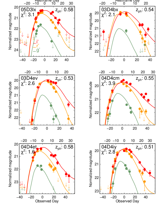
Figure 4: continued.

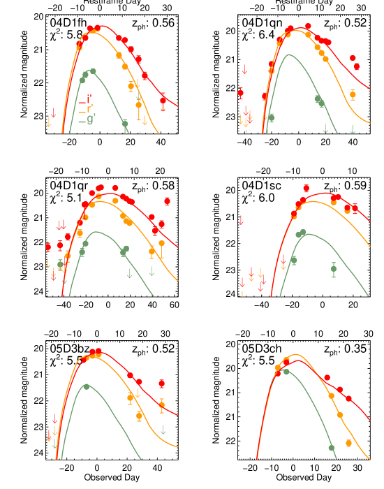
Figure 4: continued.

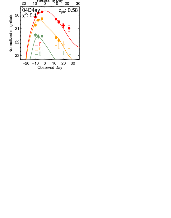
Figure 4: continued.

By using parameters derived from galaxies in our redshift range of interest, we do not need to evolve a local LF. As long as the slope of the faint end of the LF is well sampled and hence the $\alpha$ parameter is well determined, this produces an accurate luminosity density and hence an accurate SN Ia rate per unit luminosity. Figure 4 of Ilbert et al. (2005) shows that the LF in the highest redshift bin ($0.4<z<0.6$) is well sampled to $\sim$3.5 magnitudes fainter than the ‘knee’ of the function.

We now convert our volumetric rate into the commonly used luminosity specific unit called the “supernova unit” (SNu), the number of SNe per century per 10¹⁰ solar luminosities in the rest-frame B band. Dividing the luminosity density in the rest-frame B band by our volumetric rate from Table 8 gives $r_{L}=0.154^{+0.039}_{-0.031}$ SNu (statistical error only).

5.3 Systematic Errors

The rates for each field in Table 8 are all within one $\sigma_{STAT}$ of each other at each stage of the calculation of $r_{V}$. This tells us that there are no statistically significant systematic errors associated with our individual treatment of the fields. In the subsequent analysis, we examine sources of systematic error that affect the survey in its entirety. We tabulate the values and sources of statistical and systematic errors in Table 9 for both $r_{V}$ and $r_{L}$ and describe each systematic error below.

5.3.1 Spectroscopic Incompleteness

We estimate the systematic error due to spectroscopic incompleteness by using our detailed examination of the SN candidates from §3.2 as tabulated in Table 5, column 4. Using the extremes of completeness for the ensemble (75% to 100%) as limits on this systematic error, the spectroscopic incompleteness is responsible for a systematic error on $r_{V}$ of $(+0.03,-0.08)\times 10^{-4}$ yr^-1 Mpc^-3 and on $r_{L}$ of $(+0.010,-0.031)$ SNu.

5.3.2 Host Extinction

For our canonical host extinction, we used a positive valued Gaussian $E(B-V)_{h}$ distribution with a width of $\sigma_{E(B-V)_{h}}=0.2$ (see Figure 22c) combined with an extinction law with $R_{V}=3.1$ (Cardelli et al., 1989). We follow the procedure described in Sullivan et al. (2006), with the exception that our host extinction is allowed to vary beyond $E(B-V)_{h}=0.30$. Systematics are introduced if our canonical distribution differs significantly from the real SN Ia host color excess distribution, or if there is evolution of dust properties such that the $R_{V}=3.1$ model is significantly inaccurate. Preliminary results from submm surveys of SN Ia host galaxies out to redshift $z=0.5$ show no significant evolution in the dust properties when compared to hosts at $z=0.0$ (Clements et al., 2005). We thus concentrate on the distribution of $E(B-V)_{h}$ as the major source of systematic errors in our redshift range.

In an effort to quantify the systematic contribution of host extinction to an underestimation of the SN Ia rate, we re-ran our Monte Carlo efficiency experiments setting $E(B-V)_{h}=0.0$ for each simulated SN. We analyzed the results of this experiment exactly as before (see §5.1) and derived a volumetric rate of $r_{V}=0.38\pm 0.05\times 10^{-4}$ yr^-1 Mpc^-3. This rate is 10% ($0.67\sigma_{STAT}$) lower than the rate using our canonical distribution (see Table 8) and quantifies the magnitude of the error possible, if host extinction is ignored. We will also use this zero dust rate to calculate rate corrections due to host extinction (see below).

If we assume that our empirical host color excess distribution is biased by not including SNe in hosts with extreme $E(B-V)_{h}$, and hence extreme $A_{V}$, then the systematic error on $r_{V}$ is positive only. In an attempt to quantify this error, we compare our $E(B-V)_{h}$ distribution to models of SN Ia host extinction presented in Riello & Patat (2005, hereafter RP05).

RP05 improve upon the simple model of Hatano et al. (1998), motivated by the findings of Cappellaro et al. (1999) that the Hatano et al. (1998) model over-corrects the SN Ia rate in distant galaxies. RP05 use a more sophisticated model of dust distribution in SN Ia host galaxies and include the effects of varying the ratio of bulge-to-disk SNe Ia within the host. The resulting $A_{V}$ distributions, binned by inclination, are strongly peaked at $A_{V}=0.0$, have high extinction tails, and do not have a Gaussian shape (RP05, Figure 3). The smearing of the large fraction of objects with $E(B-V)_{h}\sim 0$ by photometric errors would produce a more Gaussian shape.

Because the $A_{V}$ distributions of RP05 and the $A_{B}$ distributions of Hatano et al. (1998) produce tails of objects with high extinction that extend beyond Gaussian wings, we performed two additional experiments using exponential distributions for $E(B-V)_{h}$ to simulate these tails. We generated these exponential distributions using a uniform random number generator to produce a set of random real numbers between 0 and 1, which we will designate as $\Re$, and applied the following equation:

$$E(B-V)_{h}=-\ln\Re/\lambda_{E(B-V)_{h}}\ ,$$ (5)

where $\lambda_{E(B-V)_{h}}$ is the exponential distribution scale factor. The smaller the value of $\lambda_{E(B-V)_{h}}$ the larger the tail of the distribution. Figure 23 shows the two exponential distributions with $\lambda_{E(B-V)_{h}}=5$ and $3$, along with the canonical distribution, converted to $A_{V}$ using $R_{V}=3.1$ and binned using the same bin size as RP05 ($dA_{V}=0.1$). If we compare these distributions with Figure 3 of RP05, we see that our canonical distribution is closest to the form of their model with an inclination range of $45^{\circ}\leq i\leq 60^{\circ}$. Specifically, both our distributions have a maximum of $A_{V}\sim 2.5$. The exponential distributions are closer matches to their highest inclination bin, $75^{\circ}\leq i\leq 90^{\circ}$, showing tails extending beyond $A_{V}=7.0$ (although at very low probability).

Using these distributions, we re-ran our Monte Carlo efficiency experiments and re-derived the volumetric rates to quantify the effect on our derived rate of missed SNe due to exponential tails in the host extinction distribution. For the $\lambda_{E(B-V)_{h}}=5$ distribution, we derived a rate of $r_{V}=0.44\pm 0.06\times 10^{-4}$ yr^-1 Mpc^-3, which is only 5% higher than our canonical value. The $\lambda_{E(B-V)_{h}}=3$ case produced a rate of $r_{V}=0.52\pm 0.07\times 10^{-4}$ yr^-1 Mpc^-3, which is 24% or $1.67\sigma_{STAT}$ higher. This distribution is appropriate for spiral SN Ia hosts with high inclination, but will over-estimate the correction to rates from hosts with a range of inclinations and host morphologies. We, therefore, regard it as a measure of the upper limit on the statistical error due to host extinction.

We can also compare the rate correction factors from RP05 with the correction factor resulting from the exponential dust distributions. Using our zero extinction experiment and the $\lambda_{E(B-V)_{h}}=3$ dust distribution, this factor is ${\mathcal{R}}=0.52/0.38=1.37$. This value encompasses the factors reported in RP05 (see their §5) for their models with bulge-to-total SNe ratios of $0.0\leq B/T\leq 0.5$, which are given as $1.22\leq{\mathcal{R}}_{B/T}\leq 1.31$. It also bounds their correction factors derived for dust models with $R_{V}=3.1$, $4.0$, and $5.0$ which are given as ${\mathcal{R}}_{R_{V}}=1.27,1.31,1.34$. Finally, this correction is not exceeded by the corrections derived from the RP05 models with total face-on optical depth, $\tau_{V}=0.5$ and $1.0$, which are given as ${\mathcal{R}}_{\tau_{V}}=1.16,1.27$.

These comparisons demonstrate that it is reasonable to assume that we encompass the systematic errors due to host extinction if we use the $\lambda_{E(B-V)_{h}}=3.0$ exponential host extinction distributions to define their upper limit. This results in a systematic error due to host extinction on $r_{V}$ of $(+0.10)\times 10^{-4}$ yr^-1 Mpc^-3 and on $r_{L}$ of $(+0.037)$ SNu.

5.3.3 Stretch

We consider the effect of errors in the input stretch distribution on our derived rates. We re-ran our efficiency experiment doubling the width of the stretch distribution to $\sigma_{s}=0.2$. This produced a rate of $r_{V}=0.43\pm 0.06\times 10^{-4}$ yr^-1 Mpc^-3, which is only 2% higher than the rate using $\sigma_{s}=0.1$. The resulting systematic error due to stretch for $r_{V}$ is $\pm 0.01\times 10^{-4}$ yr^-1 Mpc^-3 and for $r_{L}$ is $\pm 0.040$ SNu.

5.3.4 Frame Limits

Figure 21 shows the distribution of the 50% frame limits versus $IQ_{e}$ for a sample of $i^{\prime}$ images from the survey. The slope from Table 6, column 6 is steeper than one would expect from a simple analysis of the standard CCD $S/N$ equation (e.g., Howell 1999) in the limit where the noise is dominated by the sky (i.e. at the frame limit). The expected slope is closer to 1.3, a factor of 1.7 lower than what we derived from our fake SN experiments. This could be the result of the coaddition process, perhaps because the co-alignment accuracy is sensitive to variations in $IQ_{e}$. In order to account for a possible overestimation of the dependence of frame limit on $IQ_{e}$ (i.e. too large an $\alpha$ from equation 1), we re-ran our efficiency experiment with a constant frame limit of $i^{\prime}=24.5$, which is shown in Figure 21 as the solid horizontal line. The resulting volumetric rate was $r_{V}=0.39\pm 0.05\times 10^{-4}$ yr^-1 Mpc^-3. Using this value we estimate that an error in calculating the frame limits would introduce a systematic error on $r_{V}$ of $(-0.03)\times 10^{-4}$ yr^-1 Mpc^-3 and on $r_{L}$ of $(-0.011)$ SNu.

5.3.5 Host Offset

One of the factors offered by Dahlen et al. (2004) to account for the discrepancy between ground-based rates near $z=0.5$ and the delay-time models they present is the close proximity of SN candidates to host galaxy nuclei. If a candidate is too close to a bright host nucleus, they argue, it can be mis-classified as an AGN, or it might be passed up for spectroscopic followup because of the high level of host contamination. The results of our fake SN experiments (see §4.1, Figure 21b) show that there is no such loss of SN sensitivity close to the hosts of galaxies in the SNLS in the redshift range $0.2<z<0.6$. Another way to look at these data is shown in Figure 24, which plots the percentage of fake SN missed as a function of host offset for two $IQ_{e}$ values from our fake SN experiments (see §4.1). This further illustrates the lack of trend with host offset (see also Figure 2, Pain et al. 2002). We specifically used a brightness weighted probability distribution for placing our fake SNe, shown in Figure 24 as the dot-dashed histogram, which preferentially places them in the brightest regions of a galaxy (i.e. near the center), so that we could detect any such problem.

The study by Howell et al. (2000) also showed no significant loss of objects at small host offset when comparing a sample of 59 local SN Ia discovered with CCD detectors and a sample of 47 higher redshift ($z>0.3$) CCD-discovered SNe. We conclude that this effect is not significant, at least out to $z=0.6$, for the SNLS.

5.3.6 Subluminous SN Ia Population

Subluminous or SN 1991bg-like SNe Ia are another potential source of systematic error. Compared to the so-called normal SNe Ia these objects can have peak magnitudes up to two magnitudes fainter, exhibit different spectral features, have a different stretch color relationship, yet they still obey the stretch-luminosity relationship exhibited by the normal SNe Ia (Garnavich et al., 2004). As such, they would be useful on a Hubble diagram, however, none of our spectroscopically confirmed SNe Ia fall into the subluminous class. This has been confirmed independently by equivalent width measurements of our spectroscopically confirmed sample (Bronder, 2006). We cannot assume, however, that the relative frequency of these objects decends to zero at higher redshifts. Their intrinsic faintness and differing color may produce a bias against these objects in our followup selection criteria.

It is still likely that these subluminous SNe Ia are recent phenomena, since they are strongly associated with older stellar populations (Howell, 2001). They have yet to be found in significant numbers at redshifts beyond $z=0.2$, even though many CC SNe of similar peak magnitude have been found. It is thus reasonable to assume that the current fraction of subluminous SNe Ia forms an upper limit on the fraction at higher redshifts. The best estimate of the current fraction is from Li et al. (2001), who derive a fraction of $16\pm 6$% for the subluminious class using a volume-limited sample. Rather than attempt to evolve this number to the redshift range of interest for this study, we take the conservative approach and use it to calculate an upper limit on our systematic error due to missing the subluminous SNe Ia, assuming their relative fraction has no evolution. This calculation yields a systematic error on $r_{V}$ of $(+0.08)\times 10^{-4}$ yr^-1 Mpc^-3 and on $r_{L}$ of $(+0.029)$ SNu.

5.4 Comparison with Rates in the Literature

Figure 25 shows the same rates and SFH as Figure 1, but now with our rate included as the filled square. At $z\sim 0.45$ all four observed rates are in statistical agreement.

The result from Pain et al. (2002) at $z=0.55$ of $r_{V}=0.525^{+0.096}_{-0.086}$(stat)${}^{+0.110}_{-0.106}$(syst)$\times 10^{-4}$ yr^-1 Mpc^-3 is higher than our rate, but still in statistical agreement. We must consider that Pain et al. (2002) do not account for host extinction in their rate derivation (see their §6.8). There are two possible explanations. Either host extinction has a small effect in calculating SN Ia rates in this redshift range, or the lack of host extinction correction was compensated for by an equal amount of contamination in the result from Pain et al. (2002). If we calculate a correction for host extinction from our Monte Carlo experiment where we set all SNe to have $E(B-V)_{h}=0.0$, we can estimate how their rate would change if they had accounted for host extinction using our method. This correction is ${\mathcal{R}}=0.42/0.38=1.11$ when compared to our canonical host extinction results. Applying this 11% correction to the value from Pain et al. (2002) produces a rate of $r_{V}=0.58\times 10^{-4}$ yr^-1 Mpc^-3, which is only $0.5\sigma$ higher than their original value. We, therefore, conclude that the rates derived in this range are not significantly affected by host extinction.

5.4.1 Contamination

Even though all the rates near $z=0.5$ are in statistical agreement, the rate at $z=0.55$ from Barris & Tonry (2006) is within our redshift range and is nearly five times our value ($>4\sigma$ greater). The largest disagreement between published rates in Figure 25 (and in the literature as far as we know) is that between the rates at $z=0.55$ of Pain et al. (2002) and Barris & Tonry (2006). We point out that Barris & Tonry (2006) is a re-analysis of the data from Tonry et al. (2003), which reported a rate that agrees with Pain et al. (2002). The rate from Barris & Tonry (2006) is a factor of 3.9 higher than the rate from Pain et al. (2002). If we add the errors on these rates in quadrature, this amounts to a 3.8$\sigma$ difference.

We have shown that host extinction cannot be the sole explanation for these discrepancies. Our estimate for the host extinction correction factor for Pain et al. (2002) is ${\mathcal{R}}=1.11$, which would not be enough to resolve it. A host extinction correction factor of ${\mathcal{R}}=2.61$ would be required to bring the rate from Pain et al. (2002) just into statistical agreement with the rate of $r_{V}=2.04\pm 0.38\times 10^{-4}$ yr^-1 Mpc^-3 at $z=0.55$ from Barris & Tonry (2006). This correction is larger than the model from RP05 for hosts with total face-on optical depth of $\tau_{V}=10$ which gives ${\mathcal{R}}(\tau_{V})=2.35$, the largest correction listed in RP05. An even larger correction would be required to bring our rate into statistical agreement with the rate from Barris & Tonry (2006) at $z=0.55$. We must await deeper submm studies to see if corrections that large are reasonable for SN Ia hosts out to redshift $z=0.6$. Indications from Clements et al. (2005) are that this does not describe SN Ia hosts out to redshift $z=0.5$.

We maintain that contamination is the largest source of systematic error in SN Ia rates beyond $z=0.5$. Barris & Tonry (2006) used LCs generated from relatively sparsely sampled ($\Delta t=$ 2-3 weeks) RIZ filter photometry (Barris et al., 2004) combined with a training set of 23 spectrally identified SN Ia to verify their SN Ia sample. Dahlen et al. (2004) used low-resolution grism spectroscopy in combination with photometric methods to identify the majority of their candidate SNe Ia. Strolger et al. (2004) state that luminous SNe Ib/c can occupy nearly the same magnitude-color space as SNe Ia. Johnson & Crotts (2006) also conclude that SNe Ib/c are the biggest challenge in phototyping SNe Ia. Strolger et al. (2004) point out that the bright SNe Ib/c make up only $\sim 20\%$ of all SNe Ib/c and that SNe Ib/c make up only $\sim 30\%$ of all core-collapse (CC) SNe according to Cappellaro et al. (1999). One obvious caution is the fact that these ratios are based on a small sample ($<15$) from the local universe. Star-formation increases with redshift and it is plausible that the relative frequency of SNe Ib/c may increase as well.

We also assert that CC SNe at lower redshifts can masquerade as SNe Ia at higher redshifts. We support this assertion by pointing out Figure 9 in Sullivan et al. (2006). This figure plots photometrically determined redshifts (using a SN Ia template) against spectroscopically determined redshifts for SNe Ia and several types of CC SNe. The redshifts of the CC SNe are systematically over-estimated by as much as $\Delta z=+0.5$. Contamination of this kind is not addressed by using the typical magnitude difference between CC SNe and SNe Ia to cull out CC SNe (Richardson et al., 2002), since the CC SNe appear at the wrong redshift. This problem is strongly mitigated when host redshifts are available to cross-check SN photo-redshifts, as long as the host redshifts are reasonably accurate.

Another problem for photometric typing is reddening. As mentioned above, SNe Ia are distinguished from CC SNe in the early part of their LCs by having redder colors. Thus, a highly reddened CC SNe can appear to be a SN Ia and weeding these objects out of a SN Ia sample requires good epoch coverage of the later epochs. The SNLS has the benefit of 4 filter photometry which helps distinguish even highly reddened CC SNe early on. Even with this advantage, $\sim 10$% of our candidates promoted for spectroscopic followup turn out to be an identifiable type of CC SN (Howell et al., 2005).

The diversity of CC SNe, as compared to SNe Ia, is another challenge for photometric identification of SNe. Neither Dahlen et al. (2004) nor Barris & Tonry (2006) include a large database of spectrally identified CC SNe light curves in their training or test data sets. Until photometric methods can prove themselves convincingly against the full diversity of CC SNe, spectroscopy is the most reliable way to identify SNe. The pay-off for developing an accurate classifier based only on photometry is huge, however, given the expense of obtaining spectroscopy of SNe at high redshifts. Johnson & Crotts (2006) point out that having good spectral-energy distribution coverage and having dense time-sampling will improve the accuracy of this method, a statement that agrees with our experience with the SNLS (Sullivan et al., 2006; Guy et al., 2005).

We have emphasized the importance of verifying the majority of the SN Ia sample with spectroscopy in all of our figures comparing rates and SFH by plotting all the rates from samples that fulfill this criterion as filled symbols. Assuming these surveys have carefully characterized their spectroscopic completeness, the trend they display is the one that should be compared to SN Ia production models.

If we look in detail at the Dahlen et al. (2004) sample, we point out that the two redshift bins in which the majority of objects are spectroscopically confirmed (the ‘Gold’ objects, see Strolger et al., 2004) at $z=0.5$ (2 out of 3) and $z=1.2$ (5 out of 6) are included in our comparison of SFH and SN Ia rate evolution (see Figure 25). The other two bins have only 50% of their sample in the ‘Gold’ category: 7 out of 14 at $z=0.8$, and 1 out of 2 at $z=1.6$, and are therefore not included in this comparison.

6 Discussion

Our rest-frame SN Ia rate per unit comoving volume in the redshift range $0.2<z<0.6$ ($\langle z\rangle_{V}\simeq 0.47$) and using the cosmological parameters $\Omega_{m}=0.3$, $\Omega_{\Lambda}=0.7$ and $H_{0}=70$ km s^-1 is

$$r_{V}(\langle z\rangle_{V}=0.47)=0.42^{+0.13}_{-0.09}(syst)\pm 0.06(stat)\times 10^{-4}yr^{-1}Mpc^{-3},$$ (6)

and we also report our SN Ia rate in SNu, for comparison with previously determined rates at lower redshift:

$$r_{L}(\langle z\rangle_{V}=0.47)=0.154^{+0.048}_{-0.033}(syst)^{+0.039}_{-0.031}(stat)SNu.$$ (7)

6.1 Comparison with Star Formation History

The place to begin investigating the relationship between SFH and SN Ia production is where the systematic errors are minimized. Volumetric rates are the most appropriate to use in exploring this relationship. The SNu, defined using a blue host luminosity, is less ideal especially for SNe Ia for a number of reasons. Galaxy luminosity evolution makes interpreting trends in SNu with redshift difficult. Also, using a blue luminosity is not good for SNe Ia, since they also appear in galaxies with older and redder populations than CC SNe.

The region of minimal systematic uncertainty in the volumetric rate evolution is delineated by the trade-off between survey sensitivity and volume sampling. At low redshifts most searches are galaxy-targeted, requiring the conversion of the luminosity specific rate (SNu) to a volumetric rate through the local galaxy luminosity function. The volume sampled is low, increasing the influence of cosmic variance on the derived volumetric rate and hence, increasing the systematic errors. At high redshifts, survey sensitivity dominates the systematics since high redshift SNe are close to the detection limits, must be spectrally confirmed with lower S/N spectra, or photometrically identified with lower S/N LCs, and have projected distances that are fewer pixels from host nuclei.

For the SNLS, the redshift range $0.2<z<0.6$ is low enough to reduce systematic errors associated with detection limits, spectral confirmation, and host offset. It also samples 4 large, independent volumes of the universe minimizing the effects of cosmic variance on the errors. In our subsequent analysis, we examine two currently popular models of SN Ia production and compare them to our SN Ia rate at $\langle z\rangle_{V}=0.467$, and to the other spectroscopically confirmed rates from the literature.

6.1.1 The Two-Component Model

This recent model, first put forth by Mannucci et al. (2005) and applied to a sample of rates from the literature by Scannapieco & Bildsten (2005), proposes a delay function with two components. One component, called the prompt component, tracks SFH with a fairly short delay time ($<~{}1$ Gyr). The other component, called the extended component, is proportional to total stellar mass and has a much longer delay time. This model arose as a way to account for the high SN Ia rate in actively star-forming galaxies, relative to less active galaxies, and yet still produce the non-zero SN Ia rate in galaxies with no active star formation (Oemler & Tinsley, 1979; van den Bergh, 1990; Cappellaro et al., 1999; Mannucci et al., 2005; Sullivan et al., 2006). Gal-Yam & Maoz (2004) and Maoz & Gal-Yam (2004) observed the SN Ia rates in galaxy clusters and indicated the possibility that a long delay-time may be inconsistent with their observations, given the cluster Fe abundances. Scannapieco & Bildsten (2005) demonstrate that the Fe content of the gas in galaxy clusters can be explained by the prompt component of the two-component model. They also demonstrate that the two-component model reproduces the observed stellar [O/Fe] abundance ratios within the Galaxy (Scannapieco & Bildsten, 2005, Figure 3).

The two-component model is described by equation 1 from Scannapieco & Bildsten (2005), which gives the relationship between the cosmic star formation rate, the cosmic stellar mass and the volumetric SN Ia rate as a function of time. We re-write their equation in a more general form here:

$$r_{V}(t)=AM_{*}(t)+B\dot{M}_{*}(t),$$ (8)

which gives $A$ in terms of SNe Ia per year per unit mass and B in terms of SNe Ia per year per unit star formation. The component scaled by $A$ is the extended component, while $B$ scales the prompt component.

By comparing this model to our rate, and other spectroscopically confirmed rates from the literature, we can estimate the relative contributions of the extended and the prompt components. Figure 25 already places an upper limit of $B\lesssim 10^{-3}\ yr^{-1}(M_{\odot}\ yr^{-1})^{-1}$ because the SFH curve normalized to go through our rate represents a pure prompt component model ($A=0.0$).

Figure 26 shows a non-linear least squares fit of the spectroscopically confirmed SN Ia rates from this study (filled square) and the literature (filled circles) to the rates predicted by the two-component model using the SFH from Hopkins & Beacom (2006). This fit produces a reduced $\chi^{2}$ goodness-of-fit statistic of $\chi^{2}_{\nu}=0.361$ using the published error bars, produced by adding the statistical and systematic errors in quadrature. With 7 degrees of freedom (9 data points minus two parameters), this corresponds to a probability of 93% that the null hypothesis is correct, i.e., that the data represent a random sampling from the parent distribution described by the fit. The resulting fit parameters are $A=1.4\pm 1.0\times 10^{-14}\ yr^{-1}M_{\odot}^{-1}$ and $B=8.0\pm 2.6\times 10^{-4}\ yr^{-1}(M_{\odot}\ yr^{-1})^{-1}$ (see Figure 26).

This is the first time this model has been fit directly to volumetric rate data from the literature. Scannapieco & Bildsten (2005) normalized each component separately (using a different SFH) and then compared the resulting rate evolution to the observed rates. For the extended ($A$) component, they used the rate per unit mass for E/S0 galaxies from Mannucci et al. (2005, Table 2) which gives a value of $A=3.8^{+1.4}_{-1.2}\times 10^{-14}\ yr^{-1}M_{\odot}^{-1}$, corrected to our cosmology. An alternative value for the $A$ component can be derived from Table 3 in Mannucci et al. (2005) which gives the rate in bins of $B-K$ color, independent of morphology. The reddest bin, having $B-K>4.1$ gives $A=2.4^{+1.5}_{-1.1}\times 10^{-14}\ yr^{-1}M_{\odot}^{-1}$ (again adjusted for our cosmology), which is more consistent with the value from our fit. A possibly more important difference stems from the definition of mass. Our mass is derived from the integration of the SFH from high redshift to the epoch in question and, therefore, includes the mass from stars that have died. The mass used in Mannucci et al. (2005) was derived from the $K$-band luminosity of individual galaxies and is more representative of the mass currently in stars. Since our method tends to over-estimate the mass, our $A$ value is correspondingly lower.

For the prompt ($B$) component, Scannapieco & Bildsten (2005) first normalize the CC rate to the SFH and then use an assumed CC/SN Ia ratio, a method that they admit is highly uncertain. This produces a prompt component with $B=23\pm 10\times 10^{-4}\ yr^{-1}(M_{\odot}\ yr^{-1})^{-1}$, which is $1.45\sigma$ higher than our value. They also mention an alternate normalization using the SN Ia rate in actively star-forming galaxies as indicated by having $B-K\leq 2.6$. This method produces the value of $B=10^{+6}_{-5}\times 10^{-4}\ yr^{-1}(M_{\odot}\ yr^{-1})^{-1}$, which is consistent with our value.

We are comparing a method that normalizes the $A$ and $B$ components separately (Scannapieco & Bildsten, 2005), with a method which directly ties the component values to the rate evolution, as delineated by the rates derived from spectrally confirmed samples. Given the differences in SFH, mass definition, and method, the level of agreement is encouraging for this model. Caveats remain, however, including systematics in the lower redshift rates due to cosmic variance and systematics in the SFH. Further tests of this model will come as the SN Ia rate evolution is more precisely measured (at low and high redshifts) and as the SN Ia rate per unit mass and per unit star-formation is measured more accurately for a larger set of individual galaxies (Sullivan et al., 2006).

The success of this model implies that it is reasonable to describe SN Ia production in terms of two populations with two different delay times (see also Mannucci et al., 2006). If these two populations represent two separate channels for SN Ia production, they may also exhibit different intrinsic properties. The SNLS is carefully examining this (Sullivan et al., 2006) to avoid biases in our cosmological parameters. At higher redshifts the component tied to SFH will tend to dominate, while lower redshift samples will contain more of the extended component SNe Ia. Cosmological parameters determined with SNe Ia spanning a large range of redshifts may be subject to systematics, if unaccounted-for intrinsic differences exist.

6.1.2 Gaussian Delay Time Model

Figure 27 shows a comparison of observed rates with the delay time model delineated in Strolger et al. (2004), which is plotted as a dashed line. This model convolves the SFH with a Gaussian delay-time distribution with a characteristic delay time, $\tau$, and a width that is some fraction of the delay time: $\sigma=0.2\tau$ in this case. We updated the SFH model, using the fit from Hopkins & Beacom (2006). We find that the delay time model still fits the Dahlen et al. (2004) data with a delay time of $\tau=3$ Gyr, which is statistically consistent with the most likely value from Strolger et al. (2004). In contrast, Mannucci et al. (2006) used the data from Dahlen et al. (2004) and combined with host galaxy colors and host radio properties found a bi-modal delay distribution to be more consistent. We find that the single Gaussian model fit to the Dahlen et al. (2004) data consistently over-predicts the rates near and below $z=0.5$. In particular, the rate from Barris & Tonry (2006) at $z=0.25$ is more than $1\sigma$ below this model.

We also show a Gaussian delay time model normalized to our rate in Figure 27 as the solid line. It is statistically consistent with the spectrally confirmed SN Ia rates, except the highest one at $z=1.2$. It has the following parameters: $\tau=4.0$ Gyr and $\sigma=0.7\tau$. This model predicts a very low SN Ia rate at higher redshifts in contrast to the photometrically typed rates near a redshift of $z\sim 0.7$.

While the observations can be fit with this model, the favoured delay times tend to be longer than 3 Gyr. This is inconsistent with the finding that the SN Ia rate is much higher in galaxies with recent star formation (Oemler & Tinsley, 1979; van den Bergh, 1990; Cappellaro et al., 1999; Mannucci et al., 2005; Sullivan et al., 2006). Although we use a different set of observed rates, Mannucci et al. (2006) find that a single Gaussian delay time does not fit observed rates as a function of redshift, host color and radio loudness as well as a bi-modal delay-time distribution. If there is a strong correlation in the SN Ia rate with host galaxy star formation rate, then the overall SN Ia rate evolution should track the SFH reasonably closely, especially at higher redshifts.

The real test of the Gaussian delay model will come with rates beyond $z=1.4$ where the predicted down-turn compared to SFH will become pronounced. Our current best estimate in this range is from Dahlen et al. (2004) and is based on a sample of two SNe, only one of which was a member of the ‘Gold’ set from Strolger et al. (2004). A larger, spectroscopically confirmed sample from a much deeper survey is needed to confirm or refute this result from Dahlen et al. (2004) and therby either support or discredit the Gaussian delay-time model.

This model faces another challenge. If there is a large component of the SN Ia rate that is closely tied to the SFH, then at higher redshifts the majority of SNe Ia will arise closer to star-forming regions in their hosts. This implies that the effect of host extinction (dust) on the sensitivity of SN Ia surveys will grow with redshift. It must be shown that the downturn in the SN Ia rate measured by Dahlen et al. (2004) and predicted by this model is not the result of these factors. To do this requires the use of updated host extinction models such as RP05 combined with dust evolution models, derived from the deepest IR and submm surveys.

7 Summary

We have produced the most accurate SN Ia rate to date by using a spectroscopically confirmed sample and detection efficiencies derived from a well characterized survey. We investigated known sources of systematic errors using recent models of host extinction from RP05, and fake SN experiments to test host contamination losses. Our derived volumetric rate from a culled sample of 58 SNe Ia in the redshift range $0.2<z<0.6$ is $r_{V}=0.42^{+0.13}_{-0.09}$ (syst) $\pm 0.06$ (stat) $\times 10^{-4}$ yr^-1 Mpc^-3. We conclude from our experiments and a comparison of other rates in the literature, that contamination may be the largest source of systematic error for rates up to redshift $z=1$, in particular, for those rates based on samples that are photometrically typed.

Using the recent SFH fit from Hopkins & Beacom (2006), we compare our rate with the two-component model from Scannapieco & Bildsten (2005) and place an upper limit on the contribution from the component of SN Ia production that is closely tied to star formation of $B\lesssim 10^{-3}\ yr^{-1}(M_{\odot}\ yr^{-1})^{-1}$. By fitting this model to our rate and the spectrally confirmed rates in the literature we make an estimate of both components directly and find $A=1.4\pm 0.9\times 10^{-14}\ yr^{-1}M_{\odot}^{-1}$ and $B=8.0\pm 2.4\times 10^{-4}\ yr^{-1}(M_{\odot}\ yr^{-1})^{-1}$, with the caveat that our mass definition is an over-estimate (is the integral of SFH and, therefore, includes dead stars).

Figure 1: Observed SN Ia rate versus redshift. The filled circles are SN Ia rates derived from samples with the majority of objects confirmed by spectroscopy from the following references (in redshift order): Cappellaro et al. (1999); Madgwick et al. (2003); Blanc et al. (2004); Hardin et al. (2000); Tonry et al. (2003); Dahlen et al. (2004); Pain et al. (2002); Dahlen et al. (2004). The open circles are the SN Ia rates from Dahlen et al. (2004), whose samples employ only 50% spectroscopic confirmation. The open triangles are the rates from Barris & Tonry (2006), whose samples are confirmed almost entirely with photometric methods. The solid curve is a renormalization of the SFH from Hopkins & Beacom (2006) using a factor of $10^{3}$, which is can be considered a toy model of SN Ia production that assumes 1 SN Ia is produced instantaneously for every $10^{3}$ M_⊙ of stars formed.

Figure 2: continued.

Figure 2: continued.

Figure 2: continued.

Figure 2: continued.

Figure 2: continued.

Figure 2: continued.

Figure 2: continued.

Figure 15: Julian Date versus magnitude limit for the $i^{\prime}$ epochs in each of the four deep fields used for SN Ia detection in this study. The calendar year transitions are indicated by the vertical dashed lines. The $i^{\prime}$ magnitude limits plotted are described in §4.1.

Figure 20: Recovery percentage after human review for the two $i^{\prime}$ images having $IQ_{e}=0"\kern-4.83694pt.\kern 0.99585pt69$ (solid line) and $IQ_{e}=1"\kern-4.83694pt.\kern 0.99585pt06$ (dashed line): a) shows the total recovered percentage as a function of fake SN $i^{\prime}$ magnitude with the 50% recovery limits for each IQ shown as the vertical lines, b) - d) show the recovery fraction versus various parameters for the fake SN above the 50% recovery fractions: b) shows the recovered percentage as a function of host offset in arcseconds c) shows the total recovered percentage as a function of host minus fake SN $i^{\prime}$ magnitude, and d) shows the recovered percentage as a function of $i^{\prime}$ background measured in $i^{\prime}$ magnitudes per square arcsecond.

Figure 21: 50% detection limit as a function of $IQ_{e}$ for a range of SNLS $i^{\prime}$ images with a range of $IQ_{e}$. The $IQ_{e}$ distribution for all $i^{\prime}$ images in the survey sample time range is shown as the dashed histogram. Automated detection limits for field D1 are indicated by the open diamonds, and for field D4 by the open squares. The 50% recovery limits after human review for two D1 images at $IQ_{e}=0"\kern-4.83694pt.\kern 0.99585pt69$ and $1"\kern-4.83694pt.\kern 0.99585pt06$ are indicated by the asterisks. A linear fit to the human review limits is indicated by the bold solid line. A constant frame limit, independent of $IQ_{e}$, is indicated by the horizontal thin line at $i^{\prime}=24.5$. The human review fit and the constant limit at $i^{\prime}=24.5$ encompass all the limits shown and define the range used in our calculation of the systematic errors associated with SN Ia detection in our simulations (see §5.3).

Figure 22: Canonical distributions of properties of the simulated SNe Ia used in the Monte Carlo efficiency experiments: a) shows the volume-weighted redshift distribution as the solid histogram and the run of $dV(z)$ as the dotted line, b) shows the Gaussian stretch distribution with $\sigma=0.1$, c) shows the positive-valued Gaussian host extinction distribution with $\sigma_{E(B-V)_{h}}=0.2$, and d) shows the Gaussian $\Delta B_{MAX}$ distribution with $\sigma_{B_{MAX}}=0.17$ with a Gaussian fit overplotted as a thin solid line. The fitted $\sigma$ of the Gaussian is annotated on the plot and matches the distribution of real SNe Ia from Hamuy et al. (1996).

Figure 23: Distributions of total V-band extinction, $A_{V}$, for three models of SN Ia host extinction. The solid line represents the positive-valued Gaussian with a width of $\sigma_{E(B-V)_{h}}=0.2$ that was used for the canonical Monte Carlo efficiency experiments. The dashed line represents an exponential distribution of $E(B-V)_{h}$ with a scale parameter of $\lambda_{E(B-V)_{h}}=5.0$. The dotted line shows an exponential distribution with a scale parameter of $\lambda_{E(B-V)_{h}}=3.0$. When comparing these distributions to those in Figure 3 of Riello & Patat (2005), we see that our canonical host extinction model is appropriate for an intermediate host inclination model ($45^{\circ}\leq i\leq 60^{\circ}$), while the exponential distributions are closer to the extreme host inclination model ($75^{\circ}\leq i\leq 90^{\circ}$).

Figure 24: Percent missed versus host offset in arcseconds for $IQ_{e}=0"\kern-4.83694pt.\kern 0.99585pt69$ (solid line) and $IQ_{e}=1"\kern-4.83694pt.\kern 0.99585pt06$ (dashed line) from the fake SN experiments described in §4.1. The error bars are the Poisson errors in each bin. The histogram of the input host offsets (divided by 10) is plotted as the dot-dashed line. All data were binned with $0"\kern-4.83694pt.\kern 0.99585pt25$ bins. The percentage missed does not turn upwards at low host offset as would be expected if there was a loss of SN visibility near the host galaxy nuclei.

Figure 25: Same as Figure 1, but with the rate from this study plotted as a filled square. Because the renormalization of the SFH from Hopkins & Beacom (2006) using a factor of $10^{3}$ fits our rate, we can immediately place an upper limit on any component of SN Ia rate production that is tied directly to star formation of $r_{SFH}\lesssim 1$ SN Ia / $10^{3}$ M_⊙ ($B\lesssim 10^{-3}\ yr^{-1}(M_{\odot}\ yr^{-1})^{-1}$, see §6.1.1).

Figure 26: Fit of observed, spectrally confirmed SN Ia rates (see Figures 1 and 25) to the two component model from equation 8 shown as the solid line, with the one-sigma errors defining the shaded region. The extended ($A$) component is proportional to the current mass density, defined by integrating the SFH of Hopkins & Beacom (2006), and is shown by the dotted line, while the the prompt ($B$) component is proportional to the instantaneous SFH and is shown by the dashed line. The non-linear least-squares fit to the spectroscopically confirmed rates has $\chi^{2}_{\nu}=0.361$, and produces an extended component with $A=1.4\pm 1.0\times 10^{-14}\ yr^{-1}M_{\odot}^{-1}$ and a prompt component with $B=8.0\pm 2.6\times 10^{-4}\ yr^{-1}(M_{\odot}\ yr^{-1})^{-1}$. The errors quoted are statistical only and do not include systematics due to errors in the SFH or the mass definition.

Figure 27: Comparison of observed SN Ia rates with the delay-time model reported in Strolger et al. (2004), but using the SFH from Hopkins & Beacom (2006). The filled and open symbols are the same as in Figure 26. The dashed line is a fit to the data from Dahlen et al. (2004) with parameters of $\tau=3$ Gyr, and $\sigma=0.2\tau$. The solid line is a fit that is normalized at our rate having parameters of $\tau=4$ Gyr, and $\sigma=0.7\tau$. The fit to the data from Dahlen et al. (2004) systematically over-predicts the rates at lower redshift. Both fits predict low SN Ia rates beyond $z=1.5$.

Table 1: SNLS Observations

	Position(J2000)			Start Date			End Date		Span
Field	RA	Dec	Season	(MJD)	(YYYY-MM-DD)		(MJD)	(YYYY-MM-DD)	(days)
D1	02:26:00.00	-04:30:00.0	1	52852	2003-08-01		53026	2004-01-22	174
			2	53207	2004-07-21		53390	2005-01-20	183
D2	10:00:28.60	+02:12:21.0	1	52993	2003-12-20		53151	2004-05-26	158
			2	53328	2004-11-19		53503	2005-05-13	175
D3	14:19:28.01	+52:40:41.0	1	53017	2004-01-13		53228	2004-08-11	211
			2	53386	2005-01-16		53586	2005-08-04	200
D4	22:15:31.67	-17:44:05.0	1	52795	2003-06-05		52964	2003-11-21	169
			2	53173	2004-06-17		53350	2004-12-11	177

Table 2: Spectroscopically Confirmed Type Ia SNe: $0.2<z<0.6$

Name	$\alpha_{J2000.0}$	$\delta_{J2000.0}$	$z_{SPEC}$	Discovery (MJD)	Culling Status	Refs
SNLS-03D1ar	02:27:14.680	-04:19:05.05	0.41	52901
SNLS-03D1au	02:24:10.380	-04:02:14.96	0.50	52901		A06
SNLS-03D1aw	02:24:14.780	-04:31:01.61	0.58	52901		A06
SNLS-03D1ax	02:24:23.320	-04:43:14.41	0.50	52901		A06,H05
SNLS-03D1bp	02:26:37.720	-04:50:19.34	0.35	52913		A06,B06
SNLS-03D1dj	02:26:19.082	-04:07:09.38	0.40	52962	1-3,5	A06
SNLS-03D1fb	02:27:12.855	-04:07:16.40	0.50	52991		A06,B06
SNLS-03D1fc	02:25:43.602	-04:08:38.77	0.33	52991		A06,B06
SNLS-03D1gt	02:24:56.012	-04:07:37.08	0.55	53000	2,4	A06,B06
SNLS-04D1ag	02:24:41.108	-04:17:19.69	0.56	53019	5	A06,B06
SNLS-04D1ak	02:27:33.399	-04:19:38.73	0.53	53019		A06,B06
SNLS-04D1dc	02:26:18.477	-04:18:43.28	0.21	53228	2
SNLS-04D1hd	02:26:08.850	-04:06:35.22	0.37	53254		H05
SNLS-04D1hx	02:24:42.485	-04:47:25.38	0.56	53254
SNLS-04D1jg	02:26:12.567	-04:08:05.34	0.58	53267
SNLS-04D1kj	02:27:52.669	-04:10:49.29	0.58	53283
SNLS-04D1oh	02:25:02.372	-04:14:10.52	0.59	53294
SNLS-04D1pg	02:27:04.162	-04:10:31.35	0.51	53312
SNLS-04D1rh	02:27:47.160	-04:15:13.60	0.43	53344
SNLS-04D1sa	02:27:56.161	-04:10:34.31	0.59	53351
SNLS-04D2ac	10:00:18.924	+02:41:21.45	0.35	53022	5	A06,B06
SNLS-04D2bt	09:59:32.739	+02:14:53.22	0.22	53081	1-4	A06,B06
SNLS-04D2cf	10:01:56.048	+01:52:45.90	0.37	53081	1-4	A06,B06
SNLS-04D2cw	10:01:22.821	+02:11:55.66	0.57	53081	2-5	A06,B06
SNLS-04D2fp	09:59:28.183	+02:19:15.20	0.41	53094		A06,B06
SNLS-04D2fs	10:00:22.110	+01:45:55.64	0.36	53094		A06,B06
SNLS-04D2gb	10:02:22.712	+01:53:39.16	0.43	53094		A06
SNLS-04D2gc	10:01:39.267	+01:52:59.52	0.52	53106		A06
SNLS-04D2mh	09:59:45.872	+02:08:27.94	0.60	53356
SNLS-04D2mj	10:00:36.535	+02:34:37.44	0.51	53356
SNLS-05D2ab	10:01:50.833	+02:06:23.02	0.32	53375
SNLS-05D2ac	09:58:59.244	+02:29:22.22	0.49	53375
SNLS-05D2bv	10:02:17.008	+02:14:26.05	0.47	53391
SNLS-05D2cb	09:59:24.592	+02:19:41.34	0.43	53409
SNLS-05D2dm	10:02:07.611	+02:03:17.35	0.57	53441
SNLS-05D2dw	09:58:32.058	+02:01:56.36	0.42	53441
SNLS-05D2dy	10:00:58.083	+02:10:59.52	0.50	53441	2
SNLS-05D2ec	09:59:26.170	+02:00:49.36	0.53	53441	1,2
SNLS-05D2ei	10:01:39.103	+01:49:12.02	0.37	53441
SNLS-05D2hc	10:00:04.574	+01:53:09.94	0.36	53463
SNLS-05D2ie	10:01:02.907	+02:39:28.90	0.35	53467
SNLS-04D3df	14:18:10.020	+52:16:40.13	0.47	53110		A06
SNLS-04D3ez	14:19:07.916	+53:04:18.88	0.26	53110		A06
SNLS-04D3fk	14:18:26.212	+52:31:42.74	0.36	53117		A06
SNLS-04D3gt	14:22:32.594	+52:38:49.52	0.45	53124		A06
SNLS-04D3hn	14:22:06.878	+52:13:43.46	0.55	53124		A06,H05
SNLS-04D3kr	14:16:35.937	+52:28:44.20	0.34	53147		A06,H05
SNLS-04D3nh	14:22:26.729	+52:20:00.92	0.34	53166	1,2	A06,H05
SNLS-04D3nq	14:20:19.193	+53:09:15.90	0.22	53176		A06,H05
SNLS-05D3cf	14:16:53.369	+52:20:42.47	0.42	53410
SNLS-05D3ci	14:21:48.085	+52:26:43.33	0.51	53416
SNLS-05D3dd	14:22:30.410	+52:36:24.76	0.48	53441
SNLS-05D3gp	14:22:42.338	+52:43:28.71	0.58	53462
SNLS-05D3hq	14:17:43.058	+52:11:22.67	0.34	53474
SNLS-05D3jq	14:21:45.462	+53:01:47.53	0.58	53474
SNLS-05D3jr	14:19:28.768	+52:51:53.34	0.37	53474	1,2
SNLS-05D3kx	14:21:50.020	+53:08:13.49	0.22	53519
SNLS-05D3lq	14:21:18.449	+52:32:08.29	0.42	53528
SNLS-05D3mq	14:19:00.398	+52:23:06.81	0.24	53559	5
SNLS-05D3mx	14:22:09.078	+52:13:09.35	0.47	53559
SNLS-03D4ag	22:14:45.790	-17:44:23.00	0.28	52813		A06
SNLS-03D4au	22:16:09.920	-18:04:39.37	0.47	52815		A06,B06
SNLS-03D4cj	22:16:06.660	-17:42:16.72	0.27	52873		A06,H05
SNLS-03D4gf	22:14:22.907	-17:44:02.49	0.58	52930		A06,B06
SNLS-03D4gg	22:16:40.185	-18:09:51.82	0.59	52930		A06,B06
SNLS-03D4gl	22:14:44.177	-17:31:44.47	0.57	52935	5	A06,H05
SNLS-04D4bq	22:14:49.391	-17:49:39.37	0.55	53174		A06,B06
SNLS-04D4gg	22:16:09.268	-17:17:39.98	0.42	53228		H05
SNLS-04D4gz	22:16:59.018	-17:37:19.02	0.38	53235
SNLS-04D4ht	22:14:33.289	-17:21:31.33	0.22	53254	2
SNLS-04D4in	22:15:08.585	-17:15:39.85	0.52	53267
SNLS-04D4jr	22:14:14.335	-17:21:00.93	0.48	53284
SNLS-04D4ju	22:17:02.733	-17:19:58.34	0.47	53284

Table 3: SN Ia Sample

		Total	Culled
Field	Season	($N_{SN}$)	($N_{SN}$)
D1	1	11	8
	2	9	8
D2	1	8	4
	2	13	11
D3	1	8	7
	2	11	9
D4	1	6	5
	2	7	6
ALL		73	58

Table 4: Unconfirmed SN Ia Candidates

Name	$\alpha_{J2000.0}$	$\delta_{J2000.0}$	$z_{PHOT}$	Discovery (MJD)	Type	$\chi^{2}_{SNIa}$	Status
SNLS-03D1ge	02:24:06.043	-04:23:19.14	0.54	52993	SN?	4.208	Probable SN Ia
SNLS-04D2lu	10:01:09.465	+02:32:14.52	0.37	53353	SN?	3.741	Probable SN Ia
SNLS-04D2lx	10:01:17.159	+01:42:50.97	0.50	53353	SN?	2.031	Probable SN Ia
SNLS-04D3ht	14:16:17.101	+52:19:28.40	0.53	53135	SN?	3.129	Probable SN Ia
SNLS-05D3ba	14:18:26.790	+52:41:50.56	0.44	53387	SN?	2.323	Probable SN Ia
SNLS-05D3lc	14:22:22.902	+52:28:44.11	0.49	53519	SN	2.027	Probable SN Ia
SNLS-05D3lx	14:17:56.809	+52:20:23.26	0.58	53532	SN?	3.102	Probable SN Ia
SNLS-03D4bx	22:14:48.602	-17:31:17.58	0.54	52843	SN?	2.089	Probable SN Ia
SNLS-03D4ev	22:16:51.395	-17:20:02.37	0.53	52914	SN?	2.591	Probable SN Ia
SNLS-04D4cm	22:13:28.782	-18:03:40.56	0.55	53177	SN?	3.928	Probable SN Ia
SNLS-04D4et	22:14:51.788	-17:47:22.86	0.58	53204	SN?	1.558	Probable SN Ia
SNLS-04D4iy	22:17:07.977	-18:07:07.18	0.51	53267	SN?	2.801	Probable SN Ia
SNLS-04D1fh	02:26:59.401	-04:29:42.41	0.56	53235	SN?	5.762	Possible SN Ia
SNLS-04D1qn	02:27:28.186	-04:20:35.78	0.52	53323	SN?	6.400	Possible SN Ia
SNLS-04D1qr	02:25:49.083	-04:29:00.23	0.58	53323	SN?	5.135	Possible SN Ia
SNLS-04D1sc	02:26:34.371	-04:02:45.60	0.59	53351	SN?	6.038	Possible SN Ia
SNLS-05D3bz	14:17:50.119	+52:51:24.16	0.52	53410	SN?	5.499	Possible SN Ia
SNLS-05D3ch	14:19:09.668	+52:47:35.93	0.35	53416	SN?	5.553	Possible SN Ia
SNLS-04D4ay	22:15:54.038	-18:02:48.95	0.58	53174	SN?	5.064	Possible SN Ia

Table 5: Spectroscopic Completeness

	SNe Ia				Completeness Fraction
Field	Confirmed	Probable	Possible		Minimum	Most Likely ($C_{SPEC}$)
D1	16	1	4		0.76	0.94
D2	15	2	0		0.88	0.88
D3	16	4	2		0.73	0.80
D4	11	5	1		0.65	0.69
ALL	58	12	7		0.75	0.83

Table 6: $i^{\prime}$ Frame Limit Equation Parameters

$IQ_{GOOD}$	$IQ_{BAD}$	$E_{ref}$	$S_{ref}$	$L_{0.5}$	$\alpha$
(arcsec)	(arcsec)	(s)	(DN)	(mag)
0.69	1.06	3641	29.18	24.5	2.22

Table 7: Monte Carlo Efficiencies

	On-Field			Yearly
Field	$i^{\prime}$ Detection	Spec		Spec ($\epsilon_{yr}$)
D1	0.948	0.612		0.299
D2	0.981	0.528		0.217
D3	0.971	0.629		0.313
D4	0.979	0.654		0.310

Table 8: SNLS Type Ia SN Volumetric Rates

	$r_{RAW}$	$r_{obs}$	$r_{1+z}$	$\Theta$	$V_{\Theta,0.2<z<0.6}$	$r_{V}$
Field	(yr-1)	(yr-1)	(yr-1)	(degrees2)	($\times 10^{4}$ Mpc3)	($\times 10^{-4}$ yr-1 Mpc-3)
D1	26.7 $\pm$ 6.7	28.4 $\pm$ 7.1	41.7 $\pm$ 10.4	1.024	106.0	0.39 $\pm$ 0.10
D2	34.6 $\pm$ 8.9	39.4 $\pm$ 10.2	57.7 $\pm$ 14.9	1.026	106.2	0.54 $\pm$ 0.14
D3	25.5 $\pm$ 6.4	31.9 $\pm$ 8.0	46.8 $\pm$ 11.7	1.029	106.5	0.44 $\pm$ 0.11
D4	17.7 $\pm$ 5.3	25.7 $\pm$ 7.8	37.7 $\pm$ 11.4	1.027	106.3	0.35 $\pm$ 0.11
AVG	24.1 $\pm$ 3.3	30.3 $\pm$ 4.0	44.4 $\pm$ 5.9	1.026	106.2	0.42 $\pm$ 0.06

Table 9: Summary of Uncertainties

Source	$\delta r_{V}$	$\delta r_{L}$
Poisson	$\pm 0.06$	$\pm 0.020$
Luminosity Estimate	$\cdots$	${}^{+0.033}_{-0.023}$
Spec. Completeness	${}^{+0.03}_{-0.08}$	${}^{+0.010}_{-0.031}$
Host Extinction	$+0.10$	$+0.037$
Frame Limits	$-0.03$	$-0.011$
Stretch	$\pm 0.01$	$\pm 0.004$
Subluminous SNe Ia	$+0.08$	$+0.029$
Total Statistical	$\pm 0.06$	${}^{+0.039}_{-0.031}$
Total Systematic	${}^{+0.13}_{-0.09}$	${}^{+0.048}_{-0.033}$

References

- Astier et al. (2006) Astier, P., Guy, J., Regnault, N., Pain, R., Aubourg, E., Balam, D., Basa, S., Carlberg, R. G., Fabbro, S., Fouchez, D., Hook, I. M., Howell, D. A., Lafoux, H., Neill, J. D., Palanque-Delabrouille, N., Perrett, K., Pritchet, C. J., Rich, J., Sullivan, M., Taillet, R., Aldering, G., Antilogus, P., Arsenijevic, V., Balland, C., Baumont, S., Bronder, J., Courtois, H., Ellis, R. S., Filiol, M., Gonçalves, A. C., Goobar, A., Guide, D., Hardin, D., Lusset, V., Lidman, C., McMahon, R., Mouchet, M., Mourao, A., Perlmutter, S., Ripoche, P., Tao, C., & Walton, N. 2006, A&A, 447, 31
- Barris & Tonry (2006) Barris, B. J. & Tonry, J. L. 2006, ApJ, 637, 427
- Barris et al. (2004) Barris, B. J., Tonry, J. L., Blondin, S., Challis, P., Chornock, R., Clocchiatti, A., Filippenko, A. V., Garnavich, P., Holland, S. T., Jha, S., Kirshner, R. P., Krisciunas, K., Leibundgut, B., Li, W., Matheson, T., Miknaitis, G., Riess, A. G., Schmidt, B. P., Smith, R. C., Sollerman, J., Spyromilio, J., Stubbs, C. W., Suntzeff, N. B., Aussel, H., Chambers, K. C., Connelley, M. S., Donovan, D., Henry, J. P., Kaiser, N., Liu, M. C., Martín, E. L., & Wainscoat, R. J. 2004, ApJ, 602, 571
- Basa et al. (2006) Basa et al. 2006, in preparation
- Bertin & Arnouts (1996) Bertin, E. & Arnouts, S. 1996, A&AS, 117, 393
- Blanc et al. (2004) Blanc, G., Afonso, C., Alard, C., Albert, J. N., Aldering, G., Amadon, A., Andersen, J., Ansari, R., Aubourg, É., Balland, C., Bareyre, P., Beaulieu, J. P., Charlot, X., Conley, A., Coutures, C., Dahlén, T., Derue, F., Fan, X., Ferlet, R., Folatelli, G., Fouqué, P., Garavini, G., Glicenstein, J. F., Goldman, B., Goobar, A., Gould, A., Graff, D., Gros, M., Haissinski, J., Hamadache, C., Hardin, D., Hook, I. M., de Kat, J., Kent, S., Kim, A., Lasserre, T., Le Guillou, L., Lesquoy, É., Loup, C., Magneville, C., Marquette, J. B., Maurice, É., Maury, A., Milsztajn, A., Moniez, M., Mouchet, M., Newberg, H., Nobili, S., Palanque-Delabrouille, N., Perdereau, O., Prévot, L., Rahal, Y. R., Regnault, N., Rich, J., Ruiz-Lapuente, P., Spiro, M., Tisserand, P., Vidal-Madjar, A., Vigroux, L., Walton, N. A., & Zylberajch, S. 2004, A&A, 423, 881
- Boulade et al. (2003) Boulade, O., Charlot, X., Abbon, P., Aune, S., Borgeaud, P., Carton, P.-H., Carty, M., Da Costa, J., Deschamps, H., Desforge, D., Eppellé, D., Gallais, P., Gosset, L., Granelli, R., Gros, M., de Kat, J., Loiseau, D., Ritou, J.-., Roussé, J. Y., Starzynski, P., Vignal, N., & Vigroux, L. G. 2003, in Instrument Design and Performance for Optical/Infrared Ground-based Telescopes. Edited by Iye, Masanori; Moorwood, Alan F. M. Proceedings of the SPIE, Volume 4841, pp. 72-81 (2003), 72–81
- Bronder (2006) Bronder, J. 2006, PhD Thesis, in preparation
- Canal et al. (1996) Canal, R., Ruiz-Lapuente, P., & Burkert, A. 1996, ApJ, 456, L101
- Cappellaro et al. (1999) Cappellaro, E., Evans, R., & Turatto, M. 1999, A&A, 351, 459
- Cardelli et al. (1989) Cardelli, J. A., Clayton, G. C., & Mathis, J. S. 1989, ApJ, 345, 245
- Chandrasekhar (1931) Chandrasekhar, S. 1931, ApJ, 74, 81
- Clements et al. (2005) Clements, D. L., Farrah, D., Rowan-Robinson, M., Afonso, J., Priddey, R., & Fox, M. 2005, MNRAS, 363, 229
- Dahlen et al. (2004) Dahlen, T., Strolger, L.-G., Riess, A. G., Mobasher, B., Chary, R.-R., Conselice, C. J., Ferguson, H. C., Fruchter, A. S., Giavalisco, M., Livio, M., Madau, P., Panagia, N., & Tonry, J. L. 2004, ApJ, 613, 189
- Gal-Yam & Maoz (2004) Gal-Yam, A. & Maoz, D. 2004, MNRAS, 347, 942
- Garnavich et al. (2004) Garnavich, P. M., Bonanos, A. Z., Krisciunas, K., Jha, S., Kirshner, R. P., Schlegel, E. M., Challis, P., Macri, L. M., Hatano, K., Branch, D., Bothun, G. D., & Freedman, W. L. 2004, ApJ, 613, 1120
- Greggio (2005) Greggio, L. 2005, A&A, 441, 1055
- Guy et al. (2005) Guy, J., Astier, P., Nobili, S., Regnault, N., & Pain, R. 2005, A&A, 443, 781
- Hamuy et al. (1996) Hamuy, M., Phillips, M. M., Suntzeff, N. B., Schommer, R. A., Maza, J., & Aviles, R. 1996, AJ, 112, 2391
- Han & Podsiadlowski (2004) Han, Z. & Podsiadlowski, P. 2004, MNRAS, 350, 1301
- Hardin et al. (2000) Hardin, D., Afonso, C., Alard, C., Albert, J. N., Amadon, A., Andersen, J., Ansari, R., Aubourg, É., Bareyre, P., Bauer, F., Beaulieu, J. P., Blanc, G., Bouquet, A., Char, S., Charlot, X., Couchot, F., Coutures, C., Derue, F., Ferlet, R., Glicenstein, J. F., Goldman, B., Gould, A., Graff, D., Gros, M., Haissinski, J., Hamilton, J. C., de Kat, J., Kim, A., Lasserre, T., Lesquoy, É., Loup, C., Magneville, C., Mansoux, B., Marquette, J. B., Maurice, É., Milsztajn, A., Moniez, M., Palanque-Delabrouille, N., Perdereau, O., Prévot, L., Regnault, N., Rich, J., Spiro, M., Vidal-Madjar, A., Vigroux, L., Zylberajch, S., & The EROS Collaboration. 2000, A&A, 362, 419
- Hatano et al. (1998) Hatano, K., Branch, D., & Deaton, J. 1998, ApJ, 502, 177
- Hopkins & Beacom (2006) Hopkins, A. M. & Beacom, J. F. 2006, ApJ, submitted, astro-ph/0601463
- Howell (2001) Howell, D. A. 2001, ApJ, 554, L193
- Howell et al. (2005) Howell, D. A., Sullivan, M., Perrett, K., Bronder, T. J., Hook, I. M., Astier, P., Aubourg, E., Balam, D., Basa, S., Carlberg, R. G., Fabbro, S., Fouchez, D., Guy, J., Lafoux, H., Neill, J. D., Pain, R., Palanque-Delabrouille, N., Pritchet, C. J., Regnault, N., Rich, J., Taillet, R., Knop, R., McMahon, R. G., Perlmutter, S., & Walton, N. A. 2005, ApJ, 634, 1190
- Howell et al. (2000) Howell, D. A., Wang, L., & Wheeler, J. C. 2000, ApJ, 530, 166
- Iben & Tutukov (1984) Iben, I. & Tutukov, A. V. 1984, ApJS, 54, 335
- Ilbert et al. (2005) Ilbert, O., Tresse, L., Zucca, E., Bardelli, S., Arnouts, S., Zamorani, G., Pozzetti, L., Bottini, D., Garilli, B., Le Brun, V., Le Fèvre, O., Maccagni, D., Picat, J.-P., Scaramella, R., Scodeggio, M., Vettolani, G., Zanichelli, A., Adami, C., Arnaboldi, M., Bolzonella, M., Cappi, A., Charlot, S., Contini, T., Foucaud, S., Franzetti, P., Gavignaud, I., Guzzo, L., Iovino, A., McCracken, H. J., Marano, B., Marinoni, C., Mathez, G., Mazure, A., Meneux, B., Merighi, R., Paltani, S., Pello, R., Pollo, A., Radovich, M., Bondi, M., Bongiorno, A., Busarello, G., Ciliegi, P., Lamareille, F., Mellier, Y., Merluzzi, P., Ripepi, V., & Rizzo, D. 2005, A&A, 439, 863
- Johnson & Crotts (2006) Johnson, B. D. & Crotts, A. P. S. 2006, AJ, submitted, astro-ph/0511377
- Knop et al. (2003) Knop, R. A., Aldering, G., Amanullah, R., Astier, P., Blanc, G., Burns, M. S., Conley, A., Deustua, S. E., Doi, M., Ellis, R., Fabbro, S., Folatelli, G., Fruchter, A. S., Garavini, G., Garmond, S., Garton, K., Gibbons, R., Goldhaber, G., Goobar, A., Groom, D. E., Hardin, D., Hook, I., Howell, D. A., Kim, A. G., Lee, B. C., Lidman, C., Mendez, J., Nobili, S., Nugent, P. E., Pain, R., Panagia, N., Pennypacker, C. R., Perlmutter, S., Quimby, R., Raux, J., Regnault, N., Ruiz-Lapuente, P., Sainton, G., Schaefer, B., Schahmaneche, K., Smith, E., Spadafora, A. L., Stanishev, V., Sullivan, M., Walton, N. A., Wang, L., Wood-Vasey, W. M., & Yasuda, N. 2003, ApJ, 598, 102
- Li et al. (2001) Li, W., Filippenko, A. V., Treffers, R. R., Riess, A. G., Hu, J., & Qiu, Y. 2001, ApJ, 546, 734
- Livio (2001) Livio, M. 2001, in Supernovae and Gamma-Ray Bursts: the Greatest Explosions since the Big Bang, 334–355
- Madgwick et al. (2003) Madgwick, D. S., Hewett, P. C., Mortlock, D. J., & Wang, L. 2003, ApJ, 599, L33
- Mannucci et al. (2006) Mannucci, F., Della Valle, M., & Panagia, N. 2006, MNRAS, in press, astro-ph/0510315
- Mannucci et al. (2005) Mannucci, F., della Valle, M., Panagia, N., Cappellaro, E., Cresci, G., Maiolino, R., Petrosian, A., & Turatto, M. 2005, A&A, 433, 807
- Maoz & Gal-Yam (2004) Maoz, D. & Gal-Yam, A. 2004, MNRAS, 347, 951
- Napiwotzki et al. (2004) Napiwotzki, R., Yungelson, L., Nelemans, G., Marsh, T. R., Leibundgut, B., Renzini, R., Homeier, D., Koester, D., Moehler, S., Christlieb, N., Reimers, D., Drechsel, H., Heber, U., Karl, C., & Pauli, E.-M. 2004, in ASP Conf. Ser. 318: Spectroscopically and Spatially Resolving the Components of the Close Binary Stars, 402–410
- Nomoto (1982) Nomoto, K. 1982, ApJ, 253, 798
- Nugent et al. (2002) Nugent, P., Kim, A., & Perlmutter, S. 2002, PASP, 114, 803
- Oemler & Tinsley (1979) Oemler, A. & Tinsley, B. M. 1979, AJ, 84, 985
- Pain et al. (2002) Pain, R., Fabbro, S., Sullivan, M., Ellis, R. S., Aldering, G., Astier, P., Deustua, S. E., Fruchter, A. S., Goldhaber, G., Goobar, A., Groom, D. E., Hardin, D., Hook, I. M., Howell, D. A., Irwin, M. J., Kim, A. G., Kim, M. Y., Knop, R. A., Lee, J. C., Lidman, C., McMahon, R. G., Nugent, P. E., Panagia, N., Pennypacker, C. R., Perlmutter, S., Ruiz-Lapuente, P., Schahmaneche, K., Schaefer, B., & Walton, N. A. 2002, ApJ, 577, 120
- Pain et al. (1996) Pain, R., Hook, I. M., Deustua, S., Gabi, S., Goldhaber, G., Groom, D., Kim, A. G., Kim, M. Y., Lee, J. C., Pennypacker, C. R., Perlmutter, S., Small, I. A., Goobar, A., Ellis, R. S., McMahon, R. G., Glazebrook, K., Boyle, B. J., Bunclark, P. S., Carter, D., & Irwin, M. J. 1996, ApJ, 473, 356
- Perlmutter et al. (1999) Perlmutter, S., Aldering, G., Goldhaber, G., Knop, R. A., Nugent, P., Castro, P. G., Deustua, S., Fabbro, S., Goobar, A., Groom, D. E., Hook, I. M., Kim, A. G., Kim, M. Y., Lee, J. C., Nunes, N. J., Pain, R., Pennypacker, C. R., Quimby, R., Lidman, C., Ellis, R. S., Irwin, M., McMahon, R. G., Ruiz-Lapuente, P., Walton, N., Schaefer, B., Boyle, B. J., Filippenko, A. V., Matheson, T., Fruchter, A. S., Panagia, N., Newberg, H. J. M., Couch, W. J., & The Supernova Cosmology Project. 1999, ApJ, 517, 565
- Perrett et al. (2006) Perrett et al. 2006, in preparation
- Pritchet et al. (2006) Pritchet et al. 2006, in preparation
- Richardson et al. (2002) Richardson, D., Branch, D., Casebeer, D., Millard, J., Thomas, R. C., & Baron, E. 2002, AJ, 123, 745
- Riello & Patat (2005) Riello, M. & Patat, F. 2005, MNRAS, 362, 671, RP05
- Riess et al. (1998) Riess, A. G., Filippenko, A. V., Challis, P., Clocchiatti, A., Diercks, A., Garnavich, P. M., Gilliland, R. L., Hogan, C. J., Jha, S., Kirshner, R. P., Leibundgut, B., Phillips, M. M., Reiss, D., Schmidt, B. P., Schommer, R. A., Smith, R. C., Spyromilio, J., Stubbs, C., Suntzeff, N. B., & Tonry, J. 1998, AJ, 116, 1009
- Scannapieco & Bildsten (2005) Scannapieco, E. & Bildsten, L. 2005, ApJ, 629, L85
- Schechter (1976) Schechter, P. 1976, ApJ, 203, 297
- Strolger et al. (2004) Strolger, L.-G., Riess, A. G., Dahlen, T., Livio, M., Panagia, N., Challis, P., Tonry, J. L., Filippenko, A. V., Chornock, R., Ferguson, H., Koekemoer, A., Mobasher, B., Dickinson, M., Giavalisco, M., Casertano, S., Hook, R., Blondin, S., Leibundgut, B., Nonino, M., Rosati, P., Spinrad, H., Steidel, C. C., Stern, D., Garnavich, P. M., Matheson, T., Grogin, N., Hornschemeier, A., Kretchmer, C., Laidler, V. G., Lee, K., Lucas, R., de Mello, D., Moustakas, L. A., Ravindranath, S., Richardson, M., & Taylor, E. 2004, ApJ, 613, 200
- Sullivan et al. (2006) Sullivan, M., Howell, D. A., Perrett, K., Nugent, P. E., Astier, P., Aubourg, E., Balam, D., Basa, S., Carlberg, R. G., Conley, A., Fabbro, S., Fouchez, D., Guy, J., Hook, I., Lafoux, H., Neill, J. D., Pain, R., Palanque-Delabrouille, N., Pritchet, C. J., Regnault, N., Rich, J., Taillet, R., Aldering, G., Baumont, S., Bronder, J., Filiol, M., Knop, R. A., Perlmutter, S., & Tao, C. 2006, AJ, 131, 960
- Sullivan et al. (2006) Sullivan et al. 2006, in preparation
- Tonry et al. (2003) Tonry, J. L., Schmidt, B. P., Barris, B., Candia, P., Challis, P., Clocchiatti, A., Coil, A. L., Filippenko, A. V., Garnavich, P., Hogan, C., Holland, S. T., Jha, S., Kirshner, R. P., Krisciunas, K., Leibundgut, B., Li, W., Matheson, T., Phillips, M. M., Riess, A. G., Schommer, R., Smith, R. C., Sollerman, J., Spyromilio, J., Stubbs, C. W., & Suntzeff, N. B. 2003, ApJ, 594, 1
- Tornambe & Matteucci (1986) Tornambe, A. & Matteucci, F. 1986, MNRAS, 223, 69
- van den Bergh (1990) van den Bergh, S. 1990, PASP, 102, 1318
- Webbink (1984) Webbink, R. F. 1984, ApJ, 277, 355
- Whelan & Iben (1973) Whelan, J. & Iben, I. J. 1973, ApJ, 186, 1007
- Wood-Vasey (2005) Wood-Vasey, W. M. 2005, PhD Thesis, astro-ph/0505604
- Zwicky (1938) Zwicky, F. 1938, ApJ, 88, 529