Variable iron-line emission near the black hole of Markarian 766

Abstract

Aims. We investigate the link between ionised Fe X-ray line emission and continuum emission in a bright nearby AGN, Mrk 766.

Methods. A new long ($433$ ks) XMM-Newton observation is analysed, together with archival data from 2000 and 2001. The contribution from ionised line emission is measured and its time variations on short (5–20 ks) timescales are correlated with the continuum emission.

Results. The ionised line flux is found to be highly variable and to be strongly correlated with the continuum flux, demonstrating an origin for the ionised line emission that is co-located with the continuum emission. Most likely the emission is ionised reflection from the accretion disc within a few A.U. of the central black hole, and its detection marks the first time that such an origin has been identified other than by fitting to spectral line profiles. Future observations may be able to measure a time lag and hence achieve reverberation mapping of AGN at X-ray energies.

1 Introduction

Active galaxies are thought to be powered by accretion onto a $10^{6-9}$ M_⊙ black hole, forming an accretion disc whose hot inner region produces UV radiation. X-rays are most likely produced by inverse Compton scattering (Haardt & Maraschi, 1993). A significant fraction of the X-rays shines onto the disk, producing a “reflection spectrum”, whose main observable feature below 10 keV is Fe K$\alpha$ emission emitted by fluorescence or recombination processes at 6.4-7 keV (George & Fabian, 1991; Pounds et al., 1990). Near the black hole, gravitational redshift may lead to a broad and asymmetric emission-line profile (Fabian et al., 1989) as first observed in active galaxies with ASCA (Tanaka et al., 1995; Nandra et al., 1997). More detailed studies (e.g. Wilms et al. 2001, Reynolds et al. 2004) have since been made with XMM-Newton (Jansen et al. 2001, hereafter XMM) but have produced a puzzling result: despite the continuum X-ray source being highly time-variable, the asymmetric emission thought to be the redshifted reflected iron-line is not (Miniutti et al., 2003; Vaughan & Fabian, 2004). In some active galaxies the non-redshifted component of Fe K$\alpha$ emission has been found to be variable (e.g. Nandra et al. 2000, Vaughan & Edelson 2001), but there has so far been no strong evidence for the tight correlation between emission-line and continuum variations on short timescales that should be expected if the emitting regions are spatially co-located.

Analysis of a 2001 XMM observation of Mrk 766, a narrow-line Seyfert 1 galaxy with $z=0.0129$ (Osterbrock & Pogge, 1985), provided evidence for Fe emission shifting in energy on timescales of tens (Turner, Kraemer & Reeves, 2004) to a hundred ks (Turner et al. 2006, hereafter T06), which if interpreted as being Doppler shifts from orbiting material would place the emission $\sim 100r_{g}$ ($r_{g}=GM/c^{2}$) from the central black hole (T06). In 2005 a total of 433 ks of new data were obtained with XMM, and we present here one of the first results, the detection of variable ionised Fe-line emission that is extremely well-correlated with the continuum variations on timescales $\sim 10$ ks.

2 The observations

The datasets analysed were archived XMM observations of duration 39 ks from 2000 (Boller et al., 2001) and 129 ks from 2001 (Pounds et al., 2003) together with the new observation made during 2005 May 23 UT 19:21:51 - Jun 3 UT 21:27:10 over six XMM orbits, science observation IDs in the range 0304030[1-7]01. EPIC data utilized the medium filter and pn “PrimeSmallWindow” mode. Our analysis here describes only the pn data (Strüder et al., 2001), as these offer the best S/N ratio and were free of the photon pile-up effect. Data were processed using SAS v6.5.0. Instrument patterns 0–4 were selected. Source data were extracted from a circular cell of radius $40^{\prime\prime}$, background data from a source-free region of the same pn chip. Periods when the full-band pn count rate exceeded 2 ct/s in the background region or when the background exceeded 5% of the source count rate in the 5-10 keV band were excluded. The screening yielded an effective exposure of 402 ks over an observational baseline of $944$ ks. Mrk 766 gave a mean pn count rate 1.511$\pm 0.002$ ct/s in the 2-10 keV band. The mean screened background level was 1% of the mean source rate in this band. The 2005 mean 2-10 keV flux was $F\sim 1.3\times 10^{-11}{\rm erg\ cm^{-2}s^{-1}}$, similar to the flux in 2000 May ($F\sim 1.2\times 10^{-11}{\rm erg\ cm^{-2}s^{-1}}$) and lower than in 2001 ($F\sim 2\times 10^{-11}{\rm erg\ cm^{-2}s^{-1}}$) (Pounds et al., 2003).

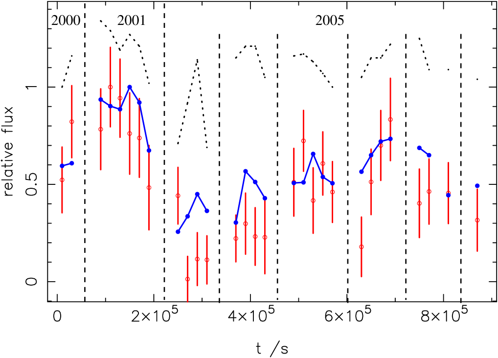
Figure 1: Light-curves for the continuum flux (blue curve, solid symbols) and emission-line flux (open, red symbols, large error bars) in the high-ionisation band (observed energy range 6.5-7.0 keV). The data are shown in independent 20 ks intervals for the pn observations from 2000, 2001 and 2005. In this figure, an artificial time interval of 40 ks has been inserted between each dataset at the times indicated by the vertical dashed lines. The flux values of each time series have been scaled to the maxima and are given as ”relative flux”. Also shown is the variation of fitted photon energy spectral index $\alpha$ (dotted line), which has values in the range $0.7<\alpha<1.4$ as indicated on the y-axis. Typical uncertainty in $\alpha$ is $\pm 0.06$.

3 Analysis of the Fe-line variations

To investigate the time variability of the Fe emission line we first fit a continuum model to the pn data over the energy range 3-9.5 keV, avoiding a strong soft-excess contribution at lower energies. The energy range 6.0-7.0 keV is excluded in order not to be biased by the Fe line emission. The model comprises a power-law of varying amplitude and slope, absorbed by cold gas (Morrison & McCammon, 1983) of variable column density. The data are divided into independently-fitted 20 ks intervals and the background spectra in each interval subtracted. Uncertainties on measured quantities include the uncertainty in the background subtraction. The line emission in any band is then estimated as the summed excess flux above the fitted continuum. We consider two bands: a “high-ionisation” band of observed energy 6.5-7.0 keV (rest energy 6.58-7.09 keV) and a “low-ionisation” band of observed energy 6.0-6.4 keV (rest energy 6.08-6.48 keV). The effects of convolution with the instrumental response (FWHM $\sim 0.14$ keV) and of possible Doppler shifts (T06) may produce some contamination between high-ionisation and low-ionisation flux in each band: for brevity, however, we use this nomenclature below.

Fig. 1 shows the variation in the emission-line flux in the high-ionisation band and the continuum, quoted in the same band, from all epochs, 2000-2005. For clarity, an artificial interval of 40 ks has been inserted between each dataset in Fig. 1. There appears a strong correlation between the continuum and high-ionisation emission-line variations. The correlation is illustrated directly in Fig. 2, which shows a clear relationship between continuum and high-ionisation emission-line flux but not between continuum and low-ionisation emission-line flux.

Figure 2: Top The correlation between continuum and emission-line flux in the high-ionisation band, observed energy range 6.5-7.0 keV, showing the same data points as in Fig. 1. The statistical uncertainty in continuum flux is much smaller than that in the line flux. Bottom The lack of correlation between continuum and emission-line flux in the low-ionisation band, observed energy range 6.0-6.4 keV.

The statistical significance of the correlation may be estimated from the Spearman rank correlation test. The rank correlation coefficient $r_{s}$ for the high-ionisation band has a value $r_{s}=0.698$ with 29 data points for the 20 ks sampling, $r_{s}=0.633$ with 57 data points for sampling at 10 ks. If the data points were independent these values would have significance levels $p=1.3\times 10^{-5}$ and $p=6.4\times 10^{-8}$: however there is measurable autocovariance in both time series which reduces the significance of the correlation between them (although photon shot noise results in the emission-line time series having an observed power spectrum that is almost flat). Hence we estimate the significance level from $10^{8}$ pairs of time series simulated from power spectra that match the data, and hence have the same autocovariance. The power spectra were estimated from a Monte-Carlo likelihood fit to the data taking into account the window function and shot noise. The simulations show that the probability of obtaining the observed correlation by chance is $p=2.3\times 10^{-5}$ for 20 ks or $p=10^{-7}$ for 10 ks sampling. If we consider instead the low-ionisation band there is no correlation (Fig. 2): for 20 ks sampling, $r_{s}=0.158$ with significance level $p=0.2$. There is weak evidence for the emission in this band being variable, with significance level $p=0.05$ from a test of $\chi^{2}$, but any variations do not appear strongly correlated with continuum flux. Inspection of the residual spectra in Fig. 3, discussed below, suggests that, although there is a narrow component of low-ionisation Fe emission, there may also be a component of broadened, possibly Doppler-shifted (T06), emission in this band during 2001.

Figure 3: Residual spectra above the fitted continuum in the range $3-9.5$ keV. Data are divided into five flux states and the residuals within each flux state co-added. Flux states increase in flux from the bottom panel to the top. Spectra are sampled at energy intervals of $0.04$ keV and smoothed with a Gaussian of FWHM $0.08$ keV to reduce shot noise without significantly degrading resolution. Lines above and below the x-axes show the rms values of the random noise (this varies between panels because of the varying amount of data incorporated into each flux state). The y-axis scale is the same on each panel.

To test the origin of the correlation we inspect the spectra of the residual flux above the fitted continuum. In each individual time interval the residual spectra are rather noisy, so to make a sensitive investigation of the residuals we divide the data into five ”flux states”, equally spaced in 2-10 keV total flux between the minimum and maximum values. Each 20 ks time interval is assigned to one of these flux states and the residual spectra in each flux state are co-added (Fig. 3). Our aim is to investigate whether there is any systematic error in the fitting procedure that may lead to a spurious correlation, and dividing into flux states in this way is a good test for this possible problem. It may be seen that the continuum has been well-fitted over the 3-9.5 keV energy range, and that there is indeed a tendency for the emission-line flux in the high-ionisation band to increase from the lowest to the highest flux states. The emission-line flux in the low-ionisation band does not show this variation, as seen in Fig. 2. There are variations in the overall emission-line profile, but we postpone more detailed modelling of the spectrum to a later paper (Turner et al. in prep.).

To further check that the ionised-band correlation is not an artefact of the continuum fitting procedure, we also consider the values of the fitted continuum model parameters and the residuals about the model. Fig. 1 also shows the value of the fitted power-law energy index. For most of the observations the fitted value is consistent with being unchanging, although a harder spectrum is found in the lowest flux state at the start of the 2005 observations. Analysis of the continuum variations indicates that this arises from the presence of a hard spectral component, visible in the lowest state in Fig. 3 that we interpret as reflection from lower-ionisation material (Turner et al., in prep.). Whether the correlation of Fig. 2 passes through the origin depends on the modelling of this component, but the strength of the correlation is unaffected by the continuum model adopted. For our purposes here we wish to use a simple model solely to measure the ”local” continuum amplitude at $\sim 6.5$ keV, not to establish its physical origin, so have used a simple power-law parameterisation of that. Repeating the correlation analysis omitting the entire orbit comprising the lowest flux state changes the correlation coefficient to $r_{s}=0.628$ with 25 data points, still significant at $p=2.8\times 10^{-4}$.

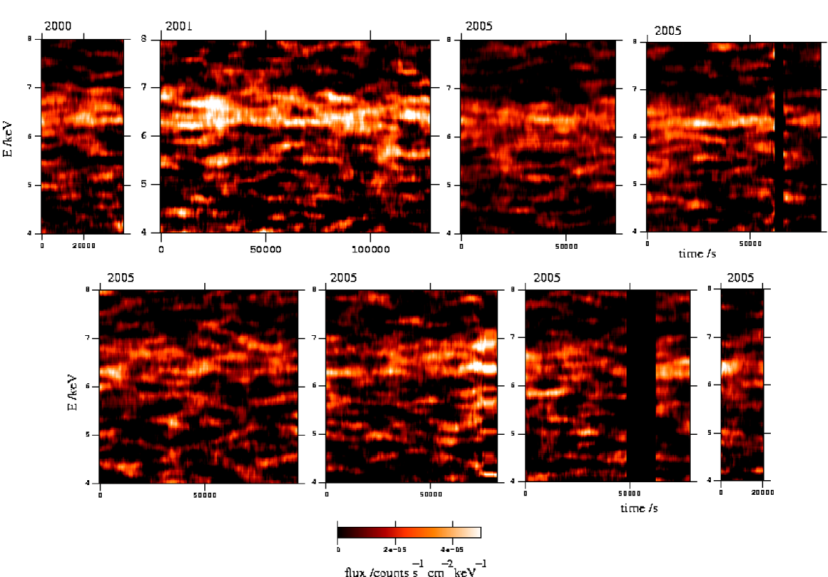
Figure 4: Colour-scale representations of the varying source spectra are shown for each observation, with the 2000 data in the upper left panel, then 2001 data, followed by six panels for the 2005 data. Photon energy is shown on the y-axis, time on the x-axis. An absorbed power-law continuum model has been fitted in 10 ks time intervals and subtracted. The scale of spectral flux density is indicated on the colour bar. The time axis has been smoothed with a top-hat of width 10 ks, the spectrum axis with a Gaussian of FWHM 0.14 keV to match the instrumental spectral resolution (see also T06). Blank regions indicate where data with high background have been removed. The strong ionised features characteristic of the 2001 data are largely absent in the 2005 data, although they appear towards the end of the fourth 2005 observation (sixth panel), coinciding with the increase in flux seen in Fig. 1.

Having established a correlation between the high-ionisation line and continuum variations, we attempt to constrain any possible time lag between the two. Such a lag would be a measure of the distance between the line- and continuum-emitting regions, as used in optical-ultraviolet “reverberation mapping”. For a circularly symmetric emission region (such as an ideal accretion disc) that is centrally illuminated the time lag is a direct measure of the radius at which the line radiation is produced. Simulations of the data yield weak evidence against the null hypothesis that there is a correlation with zero lag, with significance $p=0.11$ and a best-fitting time lag of 10 ks, corresponding to a length scale of 20 A.U., but with a 68 percent confidence interval of $\pm 10$ ks. A firmer upper limit on the lag does not exist: at larger lag values the amplitude of the window function is low (few data points overlap in the cross-correlation) and the cross-correlation error becomes large. If confirmed by further data, the existence of a lag on ks timescales would be consistent with the estimate for the emitting radius $r\sim 100r_{g}$ found when analysing the energy shifts of the Fe line in the 2001 observation (T06).

We have also searched the 2005 data for evidence of significant energy shifts, however none are found. Fig. 4 shows smoothed time-resolved spectra for the entire dataset: these spectra look very different for the 2005 data, with no evidence for the complex pattern of emission seen in the 2001 data (T06). The flux states sampled in the 2005 observation are generally significantly lower than in 2001, except for a period towards the end of the fourth orbit. Fig. 4 shows that prominent ionised-line features are only present in the highest flux states, consistent with the correlation of Fig. 2.

4 Conclusions

Detection of a line-continuum correlation on timescales of tens of ks makes it likely that the ionised Fe emission-line region is within light-hours of the continuum source in Mrk 766. The accretion disc model provides a good explanation of the general behaviour of active galaxies, and here the correlated variability and the evidence for Doppler shifts of the same gas (T06) lead us to conclude that this is indeed the expected ionised reflection from an accretion disc. The variation timescale and lack of a strongly gravitationally-redshifted asymmetric line profile implies that the ionised emission is seen at tens to hundreds of gravitational radii from the black hole. Future observations may allow better determination of a time lag and hence direct measurement of the X-ray-emitting accretion disc using reverberation mapping.

References

- Boller et al. (2001) Boller, T., Keil, R., Trümper, J. et al. 2001, A&A, 365, L146
- Fabian et al. (1989) Fabian, A.C., Rees, M.J., Stella, L., & White, N.E. 1989, MNRAS, 238, 729
- George & Fabian (1991) George, I.M. & Fabian, A.C. 1991, MNRAS, 249, 352
- Haardt & Maraschi (1993) Haardt, F. & Maraschi, L. 1993, ApJ413, 507
- Jansen et al. (2001) Jansen, F., Lumb, D., Altieri, B. et al. 2001, A&A, 365, L1
- Miniutti et al. (2003) Miniutti, G., Fabian, A.C., Goyder, R. & Lasenby, A.N. 2003, MNRAS, 344, L22
- Morrison & McCammon (1983) Morrison, R. & McCammon, D. 1983, ApJ, 270, 119
- Nandra et al. (1997) Nandra, K., George, I.M., Mushotzky, R.F., Turner, T.J. & Yaqoob,T. 1997, ApJ, 477, 602
- Nandra et al. (2000) Nandra, K., Le, T., George, I.M., Edelson, R.A. et al. 2000, ApJ, 544, 734
- Osterbrock & Pogge (1985) Osterbrock, D.E. & Pogge, R.W. 1985, ApJ, 297, 166
- Pounds et al. (1990) Pounds, K.A., Nandra, K., Stewart, G.C., George, I.M. & Fabian, A.C. 1990, Nature, 344, 132
- Pounds et al. (2003) Pounds, K.A., Reeves, J.N., Page, K.L.,Wynn, G.A. & O’Brien, P.T. 2003, MNRAS, 342, 1147
- Reynolds et al. (2004) Reynolds, C.S., Wilms, J., Begelman, M.C., Staubert, R. & Kendziorra, E., 2004, MNRAS, 349, 1153
- Strüder et al. (2001) Strüder, L., Briel, U., Dennerl, K. et al. 2001, A&A, 365, L18
- Tanaka et al. (1995) Tanaka, Y., Nandra, K., Fabian, A. et al. 1995, Nature, 375, 659
- Turner, Kraemer & Reeves (2004) Turner, T.J., Kraemer, S.B. & Reeves, J.N. 2004, ApJ, 603, 62
- Turner et al. (2006) Turner, T.J., Miller, L., Reeves, J.N. & George, I.M. 2006, A&A, 445, 59 (T06)
- Vaughan & Edelson (2001) Vaughan, S. & Edelson, R. 2001 ApJ, 548, 694
- Vaughan & Fabian (2004) Vaughan, S. & Fabian, A.C. 2004, MNRAS, 348, 1415
- Wilms et al. (2001) Wilms, J., Reynolds, C.S., Begelman, M.C. et al. 2001, MNRAS, 328, 27