Simulating the formation of molecular clouds. II. Rapid formation from turbulent initial conditions

Abstract

The characteristic lifetimes of molecular clouds remain uncertain and subject to debate, with arguments having recently been advanced in support of short-lived clouds, with lifetimes of only a few Myr, and in support of much longer-lived clouds, with lifetimes of 10 Myr or more. One argument that has been advanced in favour of long cloud lifetimes is the apparent difficulty involved in converting sufficient atomic hydrogen to molecular hydrogen within the short timescale required by the rapid cloud formation scenario. However, previous estimates of the time required for this conversion to occur have not taken into account the effects of the supersonic turbulence which is inferred to be present in the atomic gas.

In this paper, we present results from a large set of numerical simulations that demonstrate that $\rm{H}_{2}$ formation occurs rapidly in turbulent gas. Starting with purely atomic hydrogen, large quantities of molecular hydrogen can be produced on timescales of 1–2 Myr, given turbulent velocity dispersions and magnetic field strengths consistent with observations. Moreover, as our simulations underestimate the effectiveness of H₂ self-shielding and dust absorption, we can be confident that the molecular fractions that we compute are strong lower limits on the true values. The formation of large quantities of molecular gas on the timescale required by rapid cloud formation models therefore appears to be entirely plausible.

We also investigate the density and temperature distributions of gas in our model clouds. We show that the density probability distribution function is approximately log-normal, with a dispersion that agrees well with the prediction of Padoan, Nordlund & Jones (1997). The temperature distribution is similar to that of a polytrope, with an effective polytropic index $\gamma_{\rm eff}\simeq 0.8$, although at low gas densities, the scatter of the actual gas temperature around this mean value is considerable, and the polytropic approximation does not capture the full range of behaviour of the gas.

1 Introduction

An important goal of star formation research is the development of an understanding of the formation of molecular clouds, since these clouds host all observed Galactic star formation. The main constituent of these clouds is molecular hydrogen, $\rm{H}_{2}$, which forms in the interstellar medium (ISM) on the surface of dust grains, as its formation in the gas phase by radiative association occurs at a negligibly slow rate (Gould & Salpeter, 1963). The basic physics of $\rm{H}_{2}$ formation on dust is believed to be well understood, although uncertainties remain about various issues such as the relative importance of physisorption versus chemisorption (see e.g. Katz et al., 1999; Cazaux & Tielens, 2004) or the role of dust grain porosity (Perets & Biham, 2006).

However, many other questions remain unanswered. In particular, there is little consensus regarding the physical mechanism responsible for cloud formation. One school of thought holds that molecular clouds are transient objects, formed and then dispersed on a timescale of only a few million years by the action of large-scale turbulent flows in the interstellar medium (ISM), which are themselves driven by energy input from supernovae and from the magnetorotational instability (Mac Low & Klessen, 2004). Several lines of evidence in favour of this picture, such as the absence of post-T Tauri stars with ages greater than $3\>{\rm Myr}$ in local star forming regions, are discussed by Hartmann, Ballesteros-Paredes & Bergin (2001).

An alternative school of thought holds that clouds are gravitationally bound objects in virial equilibrium which evolve on timescales of the order of $10\>{\rm Myr}$ or longer, and are supported by magnetic pressure (Tassis & Mouschovias, 2004; Mouschovias et al., 2006), or by turbulence driven by the expansion of internal H ii regions(Matzner, 2002; Krumholz et al., 2006). In this picture, it is easier to reconcile the observed mass of molecular gas in the Galaxy ($M_{\rm{H}_{2}}\sim 10^{9}\>{\rm M_{\odot}}$; Evans 1999) with the inferred Galactic star formation rate ($\dot{M}_{*}\sim 3\>{\rm M_{\odot}}\>{\rm yr^{-1}}$; Scalo 1986) without requiring the average star formation efficiency of molecular clouds to be very small.

One argument often advanced in favour of longer cloud lifetimes is the apparent difficulty involved in producing sufficient $\rm{H}_{2}$ in only one or two Myr to explain observed clouds, given the relatively slow rate at which $\rm{H}_{2}$ forms in the ISM. The $\rm{H}_{2}$ formation timescale in the ISM is approximately (Hollenbach, Werner & Salpeter, 1971)

$$t_{\rm form}\simeq\frac{10^{9}\>{\rm yr}}{n},$$ (1)

where $n$ is the number density in ${\rm cm^{-3}}$, which suggests that in gas with a mean number density $\bar{n}\sim 100\>{\rm cm^{-3}}$, characteristic of most giant molecular clouds (Blitz & Shu, 1980), conversion from atomic to molecular form should take at least $10\>{\rm Myr}$, longer than the entire lifetime of a transient cloud. However, estimates of this kind do not take account of dynamical processes such as supersonic turbulence or thermal instability which may exert a great deal of influence on the effective $\rm{H}_{2}$ formation rate. The impact of these processes can be investigated through the use of numerical modelling, but in most models published to date either the dynamics of the gas have been highly simplified, with the flow restricted to one or two dimensions and with only highly ordered large-scale flows considered (see e.g. Hennebelle & Pérault, 1999, 2000; Koyama & Inutsuka, 2000, 2002; Bergin et al., 2004), or insufficient chemistry has been included to address the question at hand (e.g. Korpi et al. 1999; de Avillez 2000; Wada 2001; Kritsuk & Norman 2002a,b, 2004; Balsara et al. 2004; de Avillez & Breitschwerdt 2004; Slyz et al. 2005; Joung & Mac Low 2006).

In Glover & Mac Low (2006, hereafter paper I) we described how we have modified the publicly available ZEUS-MP hydrodynamical code (Norman, 2000) to allow us to accurately simulate the thermal balance of the atomic and molecular gas in the ISM, and to follow the growth of the molecular hydrogen fraction with time. An important feature of our approach is the use of simple approximations to treat the effects of $\rm{H}_{2}$ self-shielding and dust shielding, allowing us to approximate the $\rm{H}_{2}$ destruction rate without requiring us to solve the radiative transfer equation for the photodissociating radiation, which could only be done at a prohibitively high computational cost.

We also presented results from some simple tests of our modified code and showed that it produces physically reasonable results. Finally, we used our modified code to model molecular cloud formation by the gravitational collapse of quasi-uniform, initially static gas. We showed that in this scenario, large-scale conversion of atomic to molecular gas occurs on a timescale $t>10\>{\rm Myr}$, equivalent to at least 1–2 free-fall times (for simulations performed with our canonical value for the initial gas number density, $n_{\rm i}=100\>{\rm cm^{-3}}$).

In the current paper, we present results from a set of simulations performed with a supersonically turbulent initial velocity field, and show that the presence of turbulence dramatically reduces the time required to form large quantities of $\rm{H}_{2}$. In supersonically turbulent gas, the large density compressions created by the turbulence allow $\rm{H}_{2}$ to form rapidly, with large molecular fractions being produced after only 1–2 Myr, consistent with the timescale required by rapid cloud formation models. We also find evidence that much of the $\rm{H}_{2}$ is formed in high density gas and then transported to lower densities by the action of the turbulence, a phenomenon that may have a significant impact on the chemistry of the ISM (Xie, Allen & Langer, 1995; Willacy, Langer & Allen, 2002).

The plan of this paper is as follows. In § 2, we briefly describe the numerical method we use to simulate the gas and in § 3 we discuss the initial conditions used for our simulations. In § 4, we examine the timescale for $\rm{H}_{2}$ formation in turbulent gas, and in § 5 we analyze the resulting distribution of the molecular gas. In § 6, we discuss the temperature distribution of the gas and its evolution with time, and also examine the behaviour of the effective polytropic index, $\gamma_{\rm eff}$. In § 7 we examine how sensitive our results are to variations of our initial conditions. We conclude in § 8 with a summary of our results.

2 Numerical method

We solve the equations of fluid flow for the gas in the ISM using a modified version of the ZEUS-MP hydrodynamical code (Norman, 2000). Our modifications are based on those developed for ZEUS-3D by Pavlovski et al. (2002) and Smith & Rosen (2003), which in turn are built on earlier work by Suttner et al. (1997), and involve two major changes to the code.

First, we have added a limited treatment of non-equilibrium chemistry to the code. We treat the chemistry in an operator split fashion. During the source step, we solve the coupled set of chemical rate equations for the fluid, together with the portion of the internal energy equation dealing with compressional and radiative heating and cooling, under the assumption that the other hydrodynamical variables (e.g. density) remain fixed. During the subsequent advection step, we advect tracer fields which track the abundances of the chemical species of interest and which advect as densities, while the internal energy is advected as it would be in the unmodified version of ZEUS-MP. For stability, we solve the coupled equations implicitly, using Gauss-Seidel iteration. On the rare occasions that the iteration fails to converge, we use a more expensive bisection algorithm that is guaranteed to find a solution.

To improve the efficiency of the code, we make use of subcycling. Since the cooling time is generally much shorter than the chemical timescale for gas with the range of physical conditions of interest in this study, we evolve both the chemical rate equations and the energy equation on a cooling timestep, $\Delta t_{\rm cool}$, given by:

$$\Delta t_{\rm cool}=0.3\frac{e}{|\Lambda|},$$ (2)

where $\Lambda$ is the net rate at which the gas gains or loses energy due to radiative and chemical heating and cooling: in the convention used in our code, $\Lambda<0$ corresponds to cooling and $\Lambda>0$ to heating. Often, $\Delta t_{\rm cool}$ will be much shorter than the hydrodynamical timestep, $\Delta t_{\rm hydro}$, which is calculated as detailed in Stone & Norman (1992a). In that case, rather than constraining the code to evolve the hydrodynamics on the cooling timestep, we allow the chemistry code to subcycle: to take multiple source steps, each of length $\Delta t_{\rm cool}$, until the total elapsed time is equal to $\Delta t_{\rm hydro}$. The cooling time is recomputed following every chemistry and cooling substep, and the code also ensures that the total elapsed time cannot exceed $\Delta t_{\rm hydro}$ by shortening the last substep (if required). To further improve the efficiency of the code, our implementation of subcycling functions at the level of individual grid zones, so that only zones for which $\Delta t_{\rm cool}<\Delta t_{\rm hydro}$ are subcycled.

In our chemical model, we adopt standard solar abundances for hydrogen and helium, together with metal abundances taken from Sembach et al. (2000). We assume that metals with ionization potential less than that of atomic hydrogen (e.g. carbon, silicon) remain singly ionized throughout the calculation, and that metals with ionization potentials greater than that of hydrogen (e.g. helium, nitrogen) remain neutral. The ionization state of oxygen, which has very nearly the same ionization potential as hydrogen, is assumed to track that of hydrogen, owing to the influence of rapid charge transfer reactions. We also assume that minor ions such as $\rm{H}^{-}$, $\rm{H}_{2}^{+}$ or $\rm{H}_{3}^{+}$ can be ignored, and so are left with only four species of interest: free electrons, $\rm{H}^{+}$, $\rm{H}$ and $\rm{H}_{2}$. The abundances of these four species are constrained by two conservation laws – conservation of charge and of the number of hydrogen nuclei – and so only two of these species need to be tracked directly. We choose to follow the abundances of $\rm{H}_{2}$ and $\rm{H}^{+}$. The reactions included in our chemical model, and further details including justification of our simplifying approximations, are given in Paper I. We discuss photodissociation further below.

The second major modification to the ZEUS-MP code that we have made is to incorporate a detailed treatment of the radiative and chemical heating and cooling of the gas. The main heat source in gas with a low level of extinction is photoelectric heating (caused by the ejection of photoelectrons from dust grains and polycyclic aromatic hydrocarbons illuminated by photons with energies in the range $6<h\nu<13.6\>{\rm eV}$), while in gas with high extinction, cosmic ray heating dominates. Our treatment of these processes is based on Bakes & Tielens (1994) (as modified by Wolfire et al. 2003) and Goldsmith & Langer (1978) respectively, with the effects of extinction modelled using the approximation discussed in § 2.1 below.

The main coolants at the temperatures and densities of interest in our simulations are the fine structure lines of ${\rm C^{+}}$, ${\rm O}$ and ${\rm Si^{+}}$. We compute the cooling from these species exactly, using atomic data from a variety of sources (see Paper I). We also include heating and cooling from a variety of other processes, which are generally of lesser importance, and which are also summarized in Paper I.

2.1 ${\mathbf{H}_{2}}$ photodissociation, self-shielding and dust extinction

Following Draine & Bertoldi (1996), we assume that the $\rm{H}_{2}$ photodissociation rate can be written as the sum of an optically thin rate, $k_{\rm ph,0}$, and two separate shielding factors, $f_{\rm shield}$ and $f_{\rm dust}$ that account for the effects of $\rm{H}_{2}$ self-shielding and dust shielding respectively:

$$k_{\rm ph}=k_{\rm ph,0}f_{\rm shield}f_{\rm dust}.$$ (3)

For the optically thin rate, we adopt the expression

$$k_{\rm ph,0}=3.3\times 10^{-11}\chi\>{\rm s}^{-1},$$ (4)

where we have assumed that the ultraviolet (UV) field has the same spectral shape as the Draine (1978) field, and where $\chi$ is a dimensionless factor which characterizes the intensity of the field at $1000\>$Å relative to the Habing (1968) field; note that for the original Draine field, $\chi=1.7$.

To treat the effects of self-shielding, we use the approximation for $f_{\rm shield}$ suggested by Draine & Bertoldi (1996):

$$f_{\rm shield}=\frac{0.965}{(1+x/b_{5})^{2}}+\frac{0.035}{(1+x)^{1/2}}\exp\left[-8.5\times 10^{-4}(1+x)^{1/2}\right],$$ (5)

where $x=N_{\rm{H}_{2}}/5\times 10^{14}\>{\rm cm}^{-2}$, with $N_{\rm{H}_{2}}$ being the $\rm{H}_{2}$ column density between the fluid element and the source of the UV radiation, and with $b_{5}=b/10^{5}\>{\rm cm}\>{\rm s}^{-1}$, where $b$ is the Doppler broadening parameter.

As in paper I, we use two different approximation to compute $N_{\rm{H}_{2}}$ for every grid zone. In most of our simulations, we use a local shielding approximation. In this approximation, we assume that the dominant contribution to the self-shielding of any given fluid element comes from gas in the immediate vicinity of that element, and consequently approximate $N_{\rm{H}_{2}}$ as:

$$\tilde{N}_{\rm{H}_{2}}=\frac{\Delta x}{2}n_{\rm{H}_{2}},$$ (6)

where $n_{\rm{H}_{2}}$ is the $\rm{H}_{2}$ number density in the zone of interest and $\Delta x$ is the width of the zone, measured parallel to one of the coordinate axes. Note that since our grid zones are cubical, the choice of axis is immaterial. This approximation is intended to capture, in a crude fashion, the effects on $\rm{H}_{2}$ self-shielding of the significant Doppler shifts along any particular line of sight.

In a few simulations, however, we use an approach that we referred to in paper I as the six-ray shielding approximation. In this approach, we compute an effective $\rm{H}_{2}$ column density for each grid zone by first computing exact values along a small number of lines of sight and then averaging these values appropriately. To simplify the implementation, the lines of sight are chosen to be parallel to the coordinate axes of the grid. An approach of this type has previously been used by Nelson & Langer (1997, 1999) and Yoshida et al. (2003).

To treat shielding due to dust, we use a similar approach. We follow Draine & Bertoldi (1996) and write $f_{\rm dust}$ as

$$f_{\rm dust}=e^{-\tau_{\rm d,1000}}=e^{-\sigma_{\rm d,1000}N_{\rm\rm{H},tot}},$$ (7)

where $\tau_{\rm d,1000}$ is the optical depth due to dust at a wavelength of $1000$Å, $\sigma_{\rm d,1000}$ is the corresponding effective attenuation cross-section (which has a value $\sigma_{\rm d,1000}\simeq 2\times 10^{-21}\>{\rm cm^{2}}$ for the diffuse ISM), and $N_{\rm\rm{H},tot}$ is the total column density of hydrogen nuclei between the zone of interest and the source of the UV. To compute $N_{\rm\rm{H},tot}$, we use the same approximations as described above. In other words, when we use the local shielding approximation, we assume that the dominant contribution to $N_{\rm\rm{H},tot}$ comes from local gas, and so write it as:

$$\tilde{N}_{\rm\rm{H},tot}=\frac{\Delta x}{2}\left(n_{\rm{H}}+n_{\rm{H}^{+}}+2n_{\rm{H}_{2}}\right),$$ (8)

while in the six-ray approximation, we again compute it exactly along a small number of lines of sight.

The main advantage of our local shielding approximation (aside from its simplicity and speed) is the fact that it allows us to be certain that we are underestimating the true amount of shielding and hence overestimating the $\rm{H}_{2}$ photodissociation rate in simulations that use it. We can therefore be confident that the $\rm{H}_{2}$ fractions computed in these simulation are lower limits on the true values and hence that the timescales for $\rm{H}_{2}$ formation that we find are upper limits on the actual values. As we will see later, this fact serves to strengthen the conclusions that we draw from these simulations.

A major disadvantage of our local shielding approximation is that they make the photodissociation rate depend explicitly on the numerical resolution $\Delta x$. Consequently, the equilibrium $\rm{H}_{2}$ abundance, $x_{\rm H_{2},eq}$, also becomes resolution dependent, as can easily be seen from the following equation for $x_{\rm H_{2},eq}$

$$\frac{x_{\rm H_{2},eq}}{1-x_{\rm H_{2},eq}}=\frac{2R_{\rm form}}{R_{\rm ph}}n,$$ (9)

where $n$ is the number density of hydrogen nuclei, $R_{\rm form}$ is the formation rate of $\rm{H}_{2}$ on dust grain surfaces, $R_{\rm ph}=k_{\rm ph}n_{\rm{H}_{2}}$, and where the $\rm{H}_{2}$ abundance $x_{\rm{H}_{2}}$ is defined such that $x_{\rm{H}_{2}}=2n_{\rm{H}_{2}}/n$. It must also be said that the physical justification for treating dust shielding using the local approximation is somewhat lacking since the shielding provided by the dust should not be significantly affected by Doppler shifts along the line of sight. In paper I, we saw that for initially static, uniform density gas, these drawbacks are very serious and results obtained using the local approximation are of questionable accuracy. However, in the turbulent flows studied in the present paper, the performance of the local shielding approximation is very much better, as we will see in § 4 & 5 below.

A major disadvantage of the six-ray approximation is the extremely coarse angular resolution of the radiation field that it provides. This poor angular resolution will cause us to overestimate the amount of shielding in some regions, and underestimate it in others: the precise details will depend on the particular form of the density field, but in general we will tend to underestimate the amount of shielding whenever the volume filling factor of dense gas is small. On the other hand, the fact that this approach does not take account of velocity structure along any of the lines of sight means that it may significantly overestimate $f_{\rm shield}$ in a supersonically turbulent flow. It is therefore difficult to determine whether the amount of $\rm{H}_{2}$ produced in simulations using this method is an overestimate or an underestimate of the true amount. For the main problem that we are interested in investigating – the determination of the $\rm{H}_{2}$ formation rate in dynamically evolving, cold atomic gas – this is problematic, as it may lead us to derive an artificially short timescale for $\rm{H}_{2}$ formation. In view of this, we have adopted the local shielding approximation in most of our simulations, and have run only a few simulations using the six-ray approximation for the purposes of comparison. As we will see later, the results of these simulations agree surprisingly well with those of simulations using the local approximation.

Finally, we note that to compute the effect of the dust shielding on the photoelectric heating rate, we again use a very similar approximation: we use our value of $N_{\rm\rm{H},tot}$ computed above to calculate $A_{V}$, the extinction of the gas in the V band, and then compute the photoelectric heating rate using a radiation field strength attenuated by a factor $e^{-2.5A_{\rm V}}$, as suggested by Bergin et al. (2004).

3 Initial conditions

3.1 Box size and initial number density

Since our aim in this paper is to model the transition from atomic to molecular gas, we have chosen to consider relatively small volumes, which we visualize as being smaller sub-regions within larger, gravitationally collapsing clouds of gas, such as those found in the simulations of Kravtsov (2003) or Li, Mac Low & Klessen (2005). We therefore consider a cubical volume of size $L$, and apply periodic boundary conditions to all sides of the cube. As we discussed in paper I, in choosing a value for $L$ we aimed to strike a reasonable balance between simulating a large, representative region of a cloud (which argues for large $L$) and maximizing our physical resolution for any given numerical resolution (which argues for small $L$). For most of the simulations presented here, we settled on $L=20\>{\rm pc}$ as an appropriate value, but in § 7.1 we examine the effects of varying $L$. The value of $L$ used in each simulation is summarized in Table 1, together with the values used for our other adjustable parameters.

Within the box, we assumed an initially uniform distribution of gas, characterized by an initial number density $n_{\rm i}$. In most of our simulations, we take $n_{\rm i}=100\>{\rm cm^{-3}}$ as this value is consistent with the inferred mean densities of many observed molecular clouds (Mac Low & Klessen, 2004). However, in § 7.4 we explore the effects of reducing $n_{\rm i}$. Atomic gas with $n=100\>{\rm cm^{-3}}$ lies well within the cold neutral medium regime (Wolfire et al., 1995, 2003) and has a short cooling time ($t_{\rm cool}<0.05\>{\rm Myr}$), and so our results are insensitive to the initial temperature $T_{\rm i}$. In most of our simulations, we adopt a rather arbitrary initial temperature $T_{\rm i}=1000\>{\rm K}$, but as we demonstrate in § 6.1, simulations with $T_{\rm i}=100\>{\rm K}$ produce essentially identical results for times $t\mathbin{\lower 3.0pt\hbox{$\hbox to0.0pt{\raise 5.0pt\hbox{$\char 62\relax$}\hss}\mathchar 29208\relax$}}0.05\>{\rm Myr}$.

3.2 Magnetic field strength

Since there is now considerable observational evidence for the presence of dynamically significant magnetic fields in interstellar gas (Beck, 2001; Heiles & Crutcher, 2005), we included a magnetic field in the majority of our simulations. For simplicity, in simulations where a field was present, we assumed that it was initially uniform and oriented parallel to the $z$-axis of the simulation. The strength of the field was a free parameter, and the values used in our various simulations are summarized in Table 1. Observational determinations of the local magnetic field strength give a typical value of $6\pm 2\mu$G, and so we ensured that our fiducial value for the initial magnetic field strength, $B_{i,{\rm fid}}=5.85\mu{\rm G}$, was consistent with this value.

Our choice of this slightly odd value was motivated by our desire that the mass-to-flux ratio of the gas should be some simple multiple of the critical value (Nakano & Nakamura, 1978)

$$\left(\frac{M}{\Phi}\right)_{\rm crit}=\frac{1}{2\pi\sqrt{G}},$$ (10)

at which magnetic pressure balances gravity in an isothermal slab. For a fully atomic cloud of gas, the mass-to-flux ratio can be written in units of this critical value as (Crutcher et al., 2004)

$$\frac{M}{\Phi}=3.8\times 10^{-21}\frac{N_{\rm{H}}}{B},$$ (11)

where $N_{\rm{H}}$ is column density of atomic hydrogen in units of ${\rm cm^{-2}}$ and $B$ is the strength of the magnetic field, in units of $\mu{\rm G}$. For a simulation with a box size of $20\>{\rm pc}$ and an initial atomic hydrogen number density $n_{\rm i}=100\>{\rm cm^{-3}}$, this gives $M/\Phi=23.45/B_{i}$, where $B_{i}$ is the initial magnetic field strength (in units of $\mu{\rm G}$), and so if $B_{i}=B_{i,{\rm fid}}$, then $(M/\Phi)_{\rm fid}=4$. Observations of magnetic field strengths in molecular cloud cores, summarized in Crutcher (1999) and Crutcher et al. (2004), find a smaller mean value, $(M/\Phi)_{\rm mean}\simeq 2$, but there is significant scatter around this value, and in any case it is far from clear that we would expect to find the same value of $M/\Phi$ in dense cloud cores as we would find in the much lower density neutral atomic gas.

In addition to this fiducial case, we ran simulations with a number of other initial field strengths, as detailed in Table 1 and in § 7.2.

3.3 Initial velocity field

We generate the initial velocity field required for our simulations of turbulent gas by using the method described in Mac Low et al. (1998) and Mac Low (1999). In this method, we produce values for each component of velocity in each grid zone by drawing values from a Gaussian random field constructed to have a flat power spectrum for wavenumbers $k\equiv L/\lambda_{\rm d}$ in the range $1\leq k\leq 2$ and zero power outside of that range. The normalization of the resulting velocity field was then adjusted until the root mean square velocity, $v_{\rm rms}$, matched a previously specified initial value, $v_{\rm rms,i}$.

In most of our simulations, we set $v_{\rm rms,i}=10\>{\rm km}\>{\rm s^{-1}}$. Our choice of this value is motivated by observations of molecular clouds on scales $\sim 20\>{\rm pc}$ (Solomon et al., 1987) which find line-of-sight velocity dispersions $\sigma_{\rm los}\simeq 2$–$7\>{\rm km}\>{\rm s^{-1}}$. If due primarily to turbulent motions in the clouds, these velocity dispersions imply RMS turbulent velocities in the range $v_{\rm rms}\simeq 3.5$–$12\>{\rm km}\>{\rm s^{-1}}$. Our chosen value lies towards the top end of this range, but in § 7.3 we examine the effects of adopting smaller initial values.

Finally, it should be noted that in the simulations presented in this paper, we consider only decaying turbulence, i.e.  turbulence which is not maintained by a regular input of kinetic energy, and which therefore largely dissipates within a few turbulent crossing times (Mac Low, 1999). However, we find that significant amounts of $\rm{H}_{2}$ form within only 1–$2\>{\rm Myr}$, before the RMS velocity has decayed by more than a factor of two. We therefore anticipate that the results for driven turbulence would be quite similar. We hope to investigate this further in future work.

4 The ${\mathbf{H}_{2}}$ formation timescale

As in paper I, we first consider the formation of $\rm{H}_{2}$ in some detail in a set of fiducial simulations differing only in numerical resolution, before going on to consider in later sections the effects of changing the various input parameters. Parameters for the full set of simulations are listed in Table 1. The values we adopted for our fiducial runs are an initial density $n_{\rm i}=100\>{\rm cm^{-3}}$, an initial temperature $T_{\rm i}=1000\>{\rm K}$, an initial RMS turbulent velocity $v_{\rm rms,i}=10\>{\rm km}\>{\rm s^{-1}}$, an initial magnetic field strength $B_{\rm i}=5.85\mu{\rm G}$ and a box size $L=20\>{\rm pc}$. With these parameters, there is initially $\sim 0.1\>M_{\rm J}$ of gas in the box, but this number rapidly increases to $\sim 10\>M_{\rm J}$ as the gas cools to a thermal equilibrium temperature of approximately $65\>{\rm K}$. This initial period of cooling takes place in less than 0.05 Myr, just as in the initially static simulations discussed in paper I. This is a much shorter timescale than the turbulent crossing time of the box, $t_{\rm cross}=L/v_{\rm rms,i}\simeq 2\>{\rm Myr}$, and so the gas reaches thermal equilibrium before the turbulence has had time to strongly perturb the density structure. The initial mass-to-flux ratio of the gas in the box is $M/\Phi=4$, in units of the critical value.

We performed four runs with these parameters, with numerical resolutions of $64^{3}$, $128^{3}$, $256^{3}$ and $512^{3}$ zones, which we designate as MT64, MT128, MT256 and MT512 respectively. In Figure 1, we plot the evolution with time in these four runs of the mass-weighted mean molecular fraction, $\langle x_{\rm{H}_{2}}\rangle_{\rm M}$, defined as

$$\langle x_{\rm{H}_{2}}\rangle_{\rm M}=\frac{\sum_{i,j,k}\rho_{\rm{H}_{2}}(i,j,k)\Delta V(i,j,k)}{M_{\rm H}},$$ (12)

where $\rho_{\rm{H}_{2}}(i,j,k)$ is the mass density of $\rm{H}_{2}$ in zone $(i,j,k)$, $\Delta V(i,j,k)$ is the volume of zone $(i,j,k)$, $M_{\rm H}$ is the total mass of hydrogen present in the simulation, and where we sum over all grid zones.

Figure 1: Evolution of $\langle x_{\rm{H}_{2}}\rangle_{\rm M}$ with time in four runs with increasing numerical resolution: run MT64 (dotted line), run MT128 (dot-dashed line), run MT256 (dashed line) and run MT512 (solid line).

As Figure 1 makes clear, the $\rm{H}_{2}$ abundance evolves rapidly in turbulent gas. Large quantities of $\rm{H}_{2}$ are produced within a short time, with mass-weighted mean molecular fractions of approximately 40% being produced within only $2\>{\rm Myr}$. For comparison, in our fiducial static runs in paper I, we found that $\langle x_{\rm{H}_{2}}\rangle_{\rm M}$ exceeded 40% only for $t>30.8\>{\rm Myr}$ in the run performed using the local shielding approximation (run MS256 in the notation of paper I), and at $t>7.6\>{\rm Myr}$ in the run performed using the six-ray shielding approximation (run MS256-RT). The latter time is probably the better estimate, but even in this case there is a factor of 3–4 difference in the $\rm{H}_{2}$ formation timescale between the static and turbulent runs. Indeed, $\rm{H}_{2}$ forms significantly faster in our fiducial turbulent runs than in a static run in which there was no ultraviolet background and hence no photodissociation of $\rm{H}_{2}$ (run MS256-nr; in this run, the time at which $\langle x_{\rm{H}_{2}}\rangle_{\rm M}>0.4$ is again approximately $7.6\>{\rm Myr}$). It is also apparent from Figure 1 that although the evolution of $\langle x_{\rm{H}_{2}}\rangle_{\rm M}$ in these simulations shows some dependence on the numerical resolution of the simulation, for reasons which we will explore later, the effect is not large, and the simulations converge on very similar values for $\langle x_{\rm{H}_{2}}\rangle_{\rm M}$ after the first couple of megayears of evolution. Figure 1 therefore demonstrates one of the main results of this paper: the timescale for $\rm{H}_{2}$ formation in turbulent gas is much shorter than in quiescent gas with the same mean density and large quantities of molecular gas can be produced in turbulent regions within only a few megayears. As we will see as we proceed, we obtain qualitatively similar results for a wide range of initial conditions.

Figure 2: Evolution with time of $\rho_{\rm max}$ and $\rho_{\rm rms}$ in four runs with increasing numerical resolution: run MT64 (thick and thin dotted lines), run MT128 (thick and thin dot-dashed lines), run MT256 (thick and thin dashed lines) and run MT512 (thick and thin solid lines). Note that the time sampling of the data used to compute $\rho_{\rm rms}$ is ten times coarser than that used to compute $\rho_{\rm max}$.

Examination of the evolution of the peak density, $\rho_{\rm max}$, and the RMS density, $\rho_{\rm rms}$, in our turbulent simulations (plotted in Figure 2 with thick lines and thin lines respectively) gives us a strong hint as to why $\langle x_{\rm{H}_{2}}\rangle_{\rm M}$ grows so rapidly in turbulent gas. The turbulence very quickly produces strong compressions in the initially uniform density field, significantly increasing the RMS density of the gas within a megayear, and producing large peak densities. At times $t>1\>{\rm Myr}$, the growth in $\rho_{\rm rms}$ and $\rho_{\rm max}$ slows as the turbulence starts to become fully developed, before accelerating again at $t\sim 2\>{\rm Myr}$ (in the high resolution $256^{3}$ and $512^{3}$ runs) or $t\sim 4\>{\rm Myr}$ (in the lower resolution $64^{3}$ and $128^{3}$ runs) due to the onset of runaway gravitational collapse.

It is clear from Figure 2 that the values of $\rho_{\rm rms}$ and $\rho_{\rm max}$ that we obtain from our simulations have not converged, and therefore that the density field is not fully resolved even in our $512^{3}$ run. This is a major cause of the differences apparent in the evolution of $\langle x_{\rm{H}_{2}}\rangle_{\rm M}$ in the various runs – in the higher resolution runs, we resolve more of the dense structure, and so form more $\rm{H}_{2}$. We would expect this trend to continue as we increase the numerical resolution until we reach a point at which the flow is fully resolved. However, as discussed in § 4.3.2 of paper I, to fully resolve shocks at the densities of interest requires a physical resolution of less than 0.001 pc, which we cannot realistically achieve with a fixed grid code. Fortunately, these resolution issues do not seem to have a large impact on the values we obtain for $\langle x_{\rm{H}_{2}}\rangle_{\rm M}$ (other than in run MT64, which is very poorly resolved), suggesting that our results are not particularly sensitive to the accuracy with which we can follow the densest parts of the flow. As we shall see in § 5.1, this is probably because dense gas in our simulations quickly becomes almost fully molecular, at which point it clearly ceases to contribute significantly to the growth of $\langle x_{\rm{H}_{2}}\rangle_{\rm M}$. Hence, even fairly large errors in the computed densities in these fully molecular regions have little impact on $\langle x_{\rm{H}_{2}}\rangle_{\rm M}$.

One obvious question is whether the rapid growth in the value of $\langle x_{\rm{H}_{2}}\rangle_{\rm M}$ in our simulations is driven directly by gravitational collapse, which we expect to occur much earlier in a supersonically turbulent medium due to the density enhancements created by the turbulence, or whether it is these density enhancements alone that are responsible for the increased rate of $\rm{H}_{2}$ formation. Figure 2 suggests that at early times, it is turbulence which plays the major role, with gravitational collapse becoming important only at later times.

To investigate this point in more detail, we ran a set of simulations in which we disabled the effects of self-gravity in the code. The results of these simulations, which we denote as MT64-ng, MT128-ng, MT256-ng and MT512-ng are summarized in Table 2, while in Figure 3 we compare the evolution of $\langle x_{\rm{H}_{2}}\rangle_{\rm M}$ in the highest resolution simulation, MT512-ng, with its evolution in run MT512. From the figure it is clear that gravitational collapse is responsible for very little of the $\rm{H}_{2}$ formation seen in the simulations. Most of the $\rm{H}_{2}$ that forms in our turbulent simulations does so in dense regions that are not gravitationally bound. This is an important point, as it means that the rapid $\rm{H}_{2}$ formation that we see in our simulations is not specific to the case of gravitationally bound clouds: we would expect to see a similar effect in unbound atomic regions in which significant turbulence is present (such as the thin, dense sheets formed in the simulations of Audit & Hennebelle (2005) or Vázquez-Semadeni et al. (2006)) provided that enough gas is present to allow for effective self-shielding of the resulting $\rm{H}_{2}$. Indeed, a similar effect has been noted in a different context by Pavlovski et al. (2002), who simulate the effects of high-speed ($v_{\rm rms}>15\>{\rm km}\>{\rm s^{-1}}$), decaying turbulence in dense gas ($n=10^{6}\>{\rm cm^{-3}}$), and show that following an initial period of dissociation, the $\rm{H}_{2}$ reforms rapidly in the turbulent gas.

Figure 3: Evolution of $\langle x_{\rm{H}_{2}}\rangle_{\rm M}$ with time in two $512^{3}$ zone runs performed with and without self-gravity: run MT512 (solid line) and run MT512-ng (dashed line).

It is also important to establish how sensitive our results are to the approximations that we have made in order to treat the effects of the UV radiation field. In Figure 4a we compare the time evolution of $\langle x_{\rm{H}_{2}}\rangle_{\rm M}$ in run MT256 with its evolution in run MT256-RT, a run performed using the same initial conditions as run MT256, but which used the six-ray shielding approximation instead of the local shielding approximation. It is clear that the difference between the two runs is small. Slightly more $\rm{H}_{2}$ forms in run MT256-RT, which is just as we would expect given the greater amount of shielding in that run, but the difference between the two runs is no more than 30% at $t\simeq 3\>{\rm Myr}$. In this plot we also show how $\langle x_{\rm{H}_{2}}\rangle_{\rm M}$ evolves in the absence of an ultraviolet background, using results from run MT256-nr, which used the same initial conditions as run MT256, save that $\chi=0.0$. The results from this run are very similar to those from run MT256-RT.

Figure 4: (a) Evolution of $\langle x_{\rm{H}_{2}}\rangle_{\rm M}$ with time in three $256^{3}$ zone runs, performed using our fiducial initial conditions. In run MT256 (solid line) $\rm{H}_{2}$ photodissociation was modelled using the local shielding approximation, while in run MT256-RT (dashed line) we used the six-ray shielding approximation. Finally, in run MT256-nr (dot-dashed line), the strength of the ultraviolet background was set to zero. Note that the six-ray approximation results follow the zero radiation results very closely. (b) As (a), but for the evolution of the volume-weighted molecular fraction, $\langle x_{\rm{H}_{2}}\rangle_{\rm V}$.

This figure demonstrates that for supersonically turbulent flow, our approximations work reasonably well. At early times, the rate of growth of $\langle x_{\rm{H}_{2}}\rangle_{\rm M}$ is determined primarily by the time taken to form the $\rm{H}_{2}$, which is essentially the same in all three simulations, and so the results agree very well. At later times, $\rm{H}_{2}$ photodissociation begins to have more of an impact in run MT256, and the results of this run slowly diverge from those of runs MT256-RT and MT256-nr. The continued agreement of the latter runs indicates that there is enough shielding in run MT256-RT to make $\langle x_{\rm{H}_{2}}\rangle_{\rm M}$ almost insensitive to the value of $\chi$ (at least for the range of values examined here). It may be that the results from this run are closer to the true behaviour than the results of run MT256. However, as we cannot be certain of whether the value of $\langle x_{\rm{H}_{2}}\rangle_{\rm M}$ we obtain from run MT256-RT is an overestimate or an underestimate, whereas we can be certain that the value in run MT256 is an underestimate, we prefer to focus on the latter results, since they allow us to draw conclusions that are more robust.

A further point to investigate is how accurately our simulations can follow $\langle x_{\rm{H}_{2}}\rangle_{\rm V}$, the volume-weighted $\rm{H}_{2}$ fraction, defined as

$$\langle x_{\rm{H}_{2}}\rangle_{\rm V}=\frac{\sum_{i,j,k}x_{\rm{H}_{2}}(i,j,k)}{N},$$ (13)

where $x_{\rm{H}_{2}}(i,j,k)$ is the $\rm{H}_{2}$ fraction in the grid zone with coordinates $(i,j,k)$, and where $N$ is the total number of grid zones. In a turbulent simulation, where the distribution of mass is highly inhomogeneous (see § 5.1), $\langle x_{\rm{H}_{2}}\rangle_{\rm V}$ will be far more sensitive to the behaviour of gas in low-density regions than $\langle x_{\rm{H}_{2}}\rangle_{\rm M}$. The evolution of $\langle x_{\rm{H}_{2}}\rangle_{\rm V}$ in runs MT256, MT256-RT and MT256-nr is plotted in Figure 4b. It is clear from the figure that in this case there is more disagreement between the results obtained with our two different shielding approximations, and hence more uncertainty in the true value of $\langle x_{\rm{H}_{2}}\rangle_{\rm V}$. However, even in this case, the uncertainty is no more than a factor of two at $t\simeq 3\>{\rm Myr}$. The fact that we find better agreement for $\langle x_{\rm{H}_{2}}\rangle_{\rm M}$ than for $\langle x_{\rm{H}_{2}}\rangle_{\rm V}$ implies that our approximations do a better job of modelling the behaviour of high density, $\rm{H}_{2}$-rich regions than of low density, $\rm{H}_{2}$-poor regions. However, this is just what we expect: in regions in which $x_{\rm H_{2},eq}\sim 1$, even large errors in $f_{\rm shield}$ or $f_{\rm dust}$ will cause only small errors in the $\rm{H}_{2}$ fraction, whereas in regions with $x_{\rm H_{2},eq}\ll 1$, small errors in $f_{\rm shield}$ or $f_{\rm dust}$ can lead to large errors in the $\rm{H}_{2}$ fraction.

Finally, it is necessary to address the question of whether gravitationally unstable regions in our turbulent simulations are well-resolved. Truelove et al. (1997) showed that in order to properly resolve collapse and avoid artificial fragmentation, it is necessary to resolve the local Jeans length of the gas by at least four grid zones. In other words, collapse is resolved only while

$$\Delta x\leq\frac{1}{4}L_{\rm J}(\rho,T),$$ (14)

where $\Delta x$ is the width of a single grid zone, and $L_{\rm J}$ is the Jeans length, given by

$$L_{\rm J}=\frac{\pi^{1/2}c_{\rm s}}{\sqrt{G\rho}},$$ (15)

where $c_{\rm s}$ is the adiabatic sound speed. Since the densest gas in our simulations is also the coolest and so has the smallest sound speed, we can determine when (and if) the Truelove criterion is first violated by following the evolution with time of $L_{\rm J}$ in the grid zone with the highest gas density. We have done this for each of our simulations, and list the results in Table 2. We see that in most of our simulations, the Truelove criterion is violated within the first 1–2 Myr. This would appear to call into question our results at later times. However, as we discussed previously in paper I, the fact that we no longer properly resolve gravitational collapse in dense gas once the Truelove criterion is violated does not necessarily invalidate all of our subsequent results: the key question is how much gas is found in unresolved regions. To quantify this, we examined intermediate output dumps of density, internal energy and $\rm{H}_{2}$ fraction from each of our standard runs, determined which zones were unresolved in each case, and computed the fraction of the total gas mass in resolved regions, $f_{\rm res}$, and the fraction of the total $\rm{H}_{2}$ mass in the same resolved regions, $f_{\rm res,\rm{H}_{2}}$ for every output time for each run. The values of $f_{\rm res}$ and $f_{\rm res,\rm{H}_{2}}$ that we found at the end of each run are summarized in Table 3.

We found that in most of our simulations, we resolved zones containing more than 90% of the mass and of the $\rm{H}_{2}$ for the whole duration of the simulation, and that in our highest resolution run (MT512) we resolved more than 99.8% of the mass and 99.4% of the $\rm{H}_{2}$. The only run in which our resolution was significantly poorer than this was our lowest resolution $64^{3}$ run MT64, in which we resolve no more than 50–60% of the gas mass and $\rm{H}_{2}$ mass. We therefore argue that any errors we make in following the subsequent evolution of regions that fail to satisfy the Truelove criterion will not have a major effect on the evolution of $\langle x_{\rm{H}_{2}}\rangle_{\rm M}$ and so will not significantly alter our main conclusions.

5 ${\mathbf{H}_{2}}$ distribution

5.1 Morphology

In addition to determining the timescale for $\rm{H}_{2}$ formation, we would also like to know how the resulting $\rm{H}_{2}$ is distributed in the gas. We can get an immediate visual impression of this by looking at how $x_{\rm{H}_{2}}$ varies within a planar slice taken from the simulation volume. For example, in Figures 5a and 5b we show slices through run MT512 at time $t=1.9\>{\rm Myr}$ in the $x$-$y$ and $x$-$z$ planes respectively. We have made use of the periodic boundary conditions to orient the datacube so that both figures are centered on the zone with the largest density in the simulation. These figures demonstrate that the distribution of molecular gas in the box is highly inhomogeneous, with the largest concentrations being found in thin, filamentary structures that fill only a small fraction of the total volume. Comparison of the two figures suggests that there is a higher degree of structure in the $x$-$z$ plane than in the $x$-$y$, possibly due to the fact that the magnetic field is initially aligned parallel to the $z$-axis, but the highly ordered structure found in the simulations of magnetized collapse without turbulence analyzed in paper I is clearly absent.

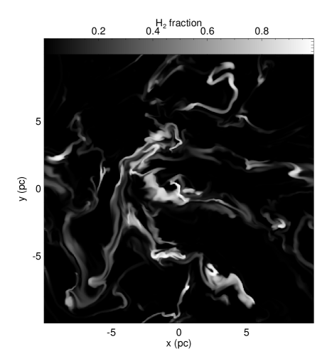
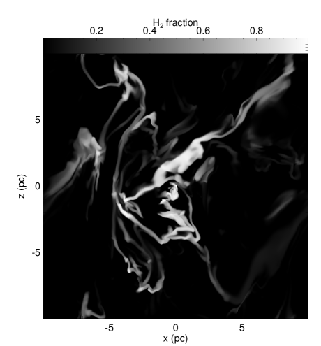
Figure 5: (a) Slice in the $x$-$y$ plane through $512^{3}$ zone run MT512 at time $t=1.9\>{\rm Myr}$ showing the spatial variation of the $\rm{H}_{2}$ fraction. We have used the fact that our simulations were performed with periodic boundary conditions to shift the image so that the zone with the highest gas density lies at the center of the figure. (b) As (a), but for a slice in the $x$-$z$ plane.

An alternative way of visualizing the $\rm{H}_{2}$ distribution is to look at the molecular gas in projection, by computing the $\rm{H}_{2}$ column density distribution that would be seen by a distant observer. In Figures 6a and 6b, we show the $\rm{H}_{2}$ column density distribution that would be seen by an observer looking along the $y$ axis or the $z$ axis respectively. These images again highlight the inhomogeneous nature of the $\rm{H}_{2}$ distribution, and also demonstrate that considerable small-scale structure exists in this distribution, despite the fact that our initial turbulent velocity field included power only on large scales.

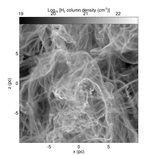
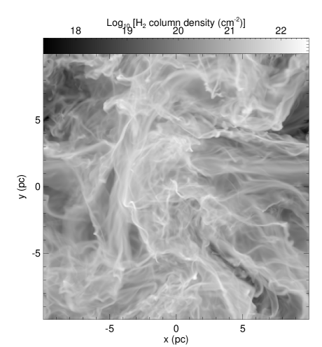
Figure 6: (a) The $\rm{H}_{2}$ column density in $512^{3}$ zone run MT512 at time $t=1.9\>{\rm Myr}$, computed for lines of sight parallel to the $y$-axis of the simulation. (b) As (a), but for lines of sight parallel to the $z$-axis.

5.2 Density dependence of the ${\mathbf{H}_{2}}$ fraction

We can study the $\rm{H}_{2}$ distribution in a more quantitative fashion by examining how the $\rm{H}_{2}$ fraction varies with density. To do this, we computed $x_{\rm{H}_{2}}$ and $n$ for each of the zones in run MT512 at $t=1.9\>{\rm Myr}$ and then binned the data by number density, using bins of width 0.05 dex. We then computed the mean and standard deviation for $x_{\rm{H}_{2}}$ in each bin. The resulting values are plotted in Figure 7. Note that although the mean values we compute here are volume weighted, we would not expect the mass weighted values to differ greatly, since the narrow width of our density bins means that there is little variation in the gas mass from zone to zone within a given bin. We also plot in Figure 7 the mean value of $x_{\rm H_{2},eq}$ for each density bin, computed using the local shielding approximation.

Figure 7: $\rm{H}_{2}$ fraction as a function of the number density of the gas (crosses) for $512^{3}$ zone run MT512 at time $t=1.9\>{\rm Myr}$. To compute these values, we binned the data by number density, using bins of width 0.05 dex, and computed the mean value of $x_{\rm{H}_{2}}$ for each bin. The standard deviation in the value of $x_{\rm{H}_{2}}$ in each bin is also indicated, as is the mean value of $x_{\rm H_{2},eq}$ for each bin (dotted line).

Three features of Figure 7 deserve particular comment. First, it is clear that there is considerable scatter in the value of $x_{\rm{H}_{2}}$ at a given density. Comparison with the plots of $x_{\rm{H}_{2}}$ versus $n$ presented in paper I for smoothly collapsing gas shows that the scatter is much greater in the turbulent case. Despite this, however, there is still an obvious underlying trend in the distribution of $x_{\rm{H}_{2}}$ with $n$, which runs in the direction that we would expect (i.e. high density gas is more highly molecular than low density gas). Second, even though $\langle x_{\rm{H}_{2}}\rangle_{\rm M}\simeq 0.4$ at this point in the simulation, there are already regions where the $\rm{H}_{2}$ fraction is very much higher, and indeed gas with a number density $n>10^{4}\>{\rm cm^{-3}}$ is already almost entirely molecular.

Finally, comparison of the distribution of $x_{\rm{H}_{2}}$ with $n$ with the equilibrium distribution (computed using the same local shielding approximation as is used in the simulation, and given by the dashed line in Figure 7) indicates that in most of the gas, the $\rm{H}_{2}$ fraction has yet to reach equilibrium. For densities in the range $300<n<10^{4}\>{\rm cm^{-3}}$, the actual $\rm{H}_{2}$ fraction lies below the equilibrium curve, indicating that the $\rm{H}_{2}$ fraction in this gas is still growing. More interestingly, in gas with $n<300\>{\rm cm^{-3}}$, the mean $x_{\rm{H}_{2}}$ lies above the equilibrium curve, implying that the $\rm{H}_{2}$ fraction in this gas must be decreasing: in other words, more $\rm{H}_{2}$ is being destroyed by photodissociation than is being formed on dust grains. To confirm that this interpretation is correct, we have computed the values of the formation and photodissociation rates of $\rm{H}_{2}$ for each grid zone in run MT512 at $t=1.9\>{\rm Myr}$. The resulting values were binned in a similar fashion to the $\rm{H}_{2}$ abundance, and the mean values in each density bin are plotted in Figure 8. As we can see, the formation rate is larger than the photodissociation rate in gas with $n>300\>{\rm cm^{-3}}$, but is smaller than the photodissociation rate in gas with $n<300\>{\rm cm^{-3}}$.

Figure 8: Mean $\rm{H}_{2}$ formation rate (solid line) and $\rm{H}_{2}$ photodissociation rate (dotted line), plotted as a function of density, for $512^{3}$ zone run MT512 at time $t=1.9\>{\rm Myr}$. For $n<300\>{\rm cm^{-3}}$, the photodissociation rate exceeds the formation rate, indicating that more $\rm{H}_{2}$ is being destroyed in this gas than is being formed in situ.

Since our simulations start with fully atomic gas, there are only two ways to explain the fact that $x_{\rm{H}_{2}}$ exceeds $x_{\rm H_{2},eq}$ at low densities: either $x_{\rm H_{2},eq}$ must have been much higher in the past, or some (or all) of the molecular content of the low density gas must have actually formed in higher density gas and then been transported to lower densities by the action of the turbulence. Of these two explanations, the first does not appear to be viable – most of the parameters that determine the value of $x_{\rm H_{2},eq}$ at a given density in our simulations (such as the strength of the UV background) are fixed, and the one parameter that does vary, the gas temperature, cannot give us the effect we seek. To demonstrate why, we have plotted in Figure 9 the variation of $x_{\rm H_{2},eq}$ with temperature for gas with a number density $n=100\>{\rm cm^{-3}}$. The mean temperature of the $100\>{\rm cm}^{-3}$ gas in our simulation is approximately $77\>{\rm K}$, and the corresponding value of $x_{\rm H_{2},eq}$ is indicated in Figure 9 by a cross. From the figure it is clear that if the temperature were slightly higher at early times in the simulation (i.e. if $T\sim 200$–300 K), then $x_{\rm H_{2},eq}$ may also have been slightly higher, but at most by about 20%. On the hand, if the temperature had been much higher, or much lower, then $x_{\rm H_{2},eq}$ would have been smaller than its present value. Given that we find a mean value of $x_{\rm{H}_{2}}$ at $n=100\>{\rm cm^{-3}}$ that is actually five times greater than the equilibrium value, it is clear that temperature variations at earlier times can be responsible for no more than a small portion of this excess, and that most or all of it must therefore be due to the transport of $\rm{H}_{2}$ from high density regions to low density regions.

Figure 9: Value of $x_{\rm H_{2},eq}$ as a function of the gas temperature $T$, computed for gas with $n=100\>{\rm cm^{-3}}$ which is shielded by a total hydrogen column density $N_{\rm\rm{H},tot}=6.0\times 10^{18}\>{\rm cm^{-2}}$. Note that this is the same amount of shielding as there would be in a zone with this value of $n$ in one of our $512^{3}$, $L=20\>{\rm pc}$ simulations. The sharp transition in $x_{\rm H_{2},eq}$ seen at $T\sim 250\>{\rm K}$ is due to the sudden onset of self-shielding: at higher temperatures, there is not enough $\rm{H}_{2}$ in the gas, even in the equilibrium state, to make the Lyman-Werner bands optically thick.

To test this hypothesis, we performed several simulations at $256^{3}$ resolution in which we artifically suppressed $\rm{H}_{2}$ formation in gas with a number density smaller than some threshold value $n_{\rm th}$. In runs MT256-th3e2, MT256-th1e3 and MT256-th3e3 we used values for $n_{\rm th}$ of 300, 1000, and $3000\>{\rm cm^{-3}}$ respectively. Our standard set of input parameters were used for all three runs. In Figure 10, we show how $\langle x_{\rm{H}_{2}}\rangle_{\rm M}$ evolves in these runs; we also plot the corresponding evolutionary track from run MT256 for comparison. Unsurprisingly, we see that as we increase $n_{\rm th}$, the total amount of $\rm{H}_{2}$ that forms in the simulations decreases. However, the reduction in $\langle x_{\rm{H}_{2}}\rangle_{\rm M}$ is less than a factor of two for $n_{\rm th}\leq 1000\>{\rm cm^{-3}}$, suggesting that most of the $\rm{H}_{2}$ that forms (and persists) in the simulation does so in the high density gas.

Figure 10: Evolution of $\langle x_{\rm{H}_{2}}\rangle_{\rm M}$ with time in $256^{3}$ zone runs MT256 (solid line), MT256-th3e2 (dashed line), MT256-th1e3 (dot-dashed line) and MT256-th3e3 (dotted line). In runs MT256-th3e2, MT256-th1e3 and MT256-th3e3, $\rm{H}_{2}$ formation was artificially suppressed in gas with a number density $n<n_{\rm th}=300$, 1000, and $3000\>{\rm cm^{-3}}$, respectively.

To examine how the $\rm{H}_{2}$ in these simulations is distributed with density, we computed the mean value of $x_{\rm{H}_{2}}$ in a set of density bins of width 0.05 dex in all three runs at time $t=1.9\>{\rm Myr}$, and compared the values with those previously computed for run MT256. The results are plotted in Figure 11; for clarity, we do not indicate the size of the standard deviations in these values, although they are comparable to those in Figure 7.

Figure 11: $\rm{H}_{2}$ fraction as a function of gas number density at $t=1.9\>{\rm Myr}$ in $256^{3}$ zone runs MT256 (solid line), MT256-th3e2 (short-dashed line), MT256-th1e3 (dot-dashed line) and MT256-th3e3 (long-dashed line). No $\rm{H}_{2}$ can form in these runs at densities $n<n_{\rm th}$, where $n_{\rm th}=0$, 300, 1000 and $3000\>{\rm cm^{-3}}$, respectively, which means that $\rm{H}_{2}$ present at $n<n_{\rm th}$ must have initially formed in denser gas. For reference, we also indicate the mean value of $x_{\rm H_{2},eq}$ as a function of number density in run MT256 (dotted line).

There are two important conclusions that we can draw from this figure. First, it is clear that although the imposition of a density threshold for $\rm{H}_{2}$ formation substantially reduces the amount of $\rm{H}_{2}$ present in gas with $n<n_{\rm th}$, it does not eliminate it: some $\rm{H}_{2}$ remains, and since it cannot have formed in situ in these simulations, it must have formed in higher density gas and been transported to the low density gas by the turbulent velocity field. Second, imposing a density threshold also affects the $\rm{H}_{2}$ abundance at densities above the threshold: although the results of the various runs eventually converge at high density, there are clear differences for densities $n\mathbin{\lower 3.0pt\hbox{$\hbox to0.0pt{\raise 5.0pt\hbox{$\char 60\relax$}\hss}\mathchar 29208\relax$}}3n_{\rm th}$, rather than at $n\mathbin{\lower 3.0pt\hbox{$\hbox to0.0pt{\raise 5.0pt\hbox{$\char 60\relax$}\hss}\mathchar 29208\relax$}}n_{\rm th}$ as we might have initially expected.

In retrospect, this behaviour should perhaps have been expected. Since the $\rm{H}_{2}$ formation rate scales as the square of the number density, $n^{2}$, overdense gas makes a disproportionately large contribution to the overall $\rm{H}_{2}$ formation rate compared to underdense gas or gas with densities near the mean value. However, previous numerical work on isothermal turbulence has shown that many of the overdense structures formed in supersonically turbulent flows are transient objects with short lifetimes (see e.g. Klessen, Heitsch & Mac Low, 2000; Vázquez-Semadeni et al., 2005). Therefore, any $\rm{H}_{2}$ formed within these transient overdensities will not remain at high densities for long, but will quite quickly find itself carried into much lower density surroundings. The results of runs MT256-th3e2, MT256-th1e3 and MT256-th3e3 suggest that a large fraction of the $\rm{H}_{2}$ in the gas is produced in this fashion.

It would clearly be of great interest to determine the extent to which $\rm{H}_{2}$ formed in transient overdensities is actually mixed into lower density material as the overdensities expand and are broken up by the flow; i.e. the amount of turbulent mixing of material which occurs. Unfortunately, to determine this with an Eulerian code such as ZEUS-MP, we would need to use tracer particles to follow individual fluid elements and these are not currently implemented in our version of the code. We intend to revisit this issue in future work.

Finally, we have investigated how sensitive our results on the density distribution of $\rm{H}_{2}$ are to the choice of shielding approximation. In Figure 12 we plot $x_{\rm{H}_{2}}$ as a function of $n$ in runs MT256 and MT256-RT at time $t=1.9\>{\rm Myr}$. Above $n=1000\>{\rm cm^{-3}}$, the results of these two runs are almost indistinguishable. Since, as we have just seen, the majority of $\rm{H}_{2}$ in these simulations forms at densities $n>1000\>{\rm cm^{-3}}$, this provides a simple explanation for the insensitivity of $\langle x_{\rm{H}_{2}}\rangle_{\rm M}$ to our choice of shielding approximation. At lower densities, the difference between runs MT256 and MT256-RT is greater. However, for $100<n<1000\>{\rm cm^{-3}}$, the mean value of $x_{\rm{H}_{2}}$ derived in run MT256-RT lies within the range of values found in run MT256, and the two runs only differ significantly at $n<100\>{\rm cm^{-3}}$. In run MT256, the $\rm{H}_{2}$ fraction at $n<100\>{\rm cm^{-3}}$ very quickly falls to almost zero, as there is not enough shielding at these densities to maintain a large $\rm{H}_{2}$ fraction. In run MT256-RT, on the other hand, shielding by the surrounding gas enables $\rm{H}_{2}$ to survive in some regions, even at these low densities, producing the extended tail seen in the distribution.

Figure 12: $\rm{H}_{2}$ fraction as a function of the number density of the gas for $256^{3}$ zone runs MT256 (crosses) and MT256-RT (squares) at time $t=1.9\>{\rm Myr}$. The standard deviation in the value of $x_{\rm{H}_{2}}$ in each bin is also indicated.

5.3 Density probability distribution function and cumulative mass function

We can further characterize the $\rm{H}_{2}$ distribution produced in our simulations by determining at which densities the bulk of the molecular gas resides. We have already seen that the highest molecular fractions are found in the densest gas, but in order to quantify how much of the total molecular mass is located at high densities, we need to characterize the density distribution of the gas. To do this, we have computed the mass-weighted density probability function (PDF) for run MT512 at $t=1.9\>{\rm Myr}$ (plotted in Figure 13). For ease of comparison with other values in the literature, we plot the PDF here as a function of $s=\ln(n/n_{\rm i})$, where $n_{\rm i}=100\>{\rm cm^{-3}}$ is the mean number density of hydrogen nuclei, which in our simulations is identically equal to the initial number density of hydrogen nuclei. We also plot in Figure 13 a log-normal function of the form

$$p_{\rm m}(s)=\frac{1}{\sqrt{2\pi\sigma^{2}}}\exp\left[-\frac{(s-s_{\rm m})^{2}}{2\sigma^{2}}\right],$$ (16)

where $s_{\rm m}$ and $\sigma$ are the mean and dispersion of the log-normal distribution, respectively; note that these are related by $|s_{\rm m}|=\sigma^{2}/2$. To construct the log-normal distribution in Figure 13 we have set $s_{\rm m}=1.32$, which is the mean of the actual dataset. Figure 13 demonstrates that at densities above the mean ($s>0$), the density PDF of run MT512 is close to a log-normal in form. On the other hand, at densities below the mean, clear deviations from a log-normal are apparent: there is a pronounced excess of power at $s=-2$, corresponding to $n\simeq 10\>{\rm cm^{-3}}$, and a deficit of power at lower densities. Previous investigations by Passot & Váquez-Semadeni (1998) and Scalo et al. (1998) of the influence of the polytropic exponent $\gamma$ on the shape of the density PDF produced by a turbulent flow suggested that a highly turbulent flow with $\gamma<1$ should produce a power-law density PDF at densities above the mean, and that a log-normal PDF is only recovered if $\gamma=1$; i.e. if the gas is isothermal. However, this prediction is based primarily on the results from one-dimensional simulations and the predicted behaviour is not seen in the three-dimensional simulations of Li, Klessen & Mac Low (2003) or Mac Low et al. (2005). Our simulations have an effective polytropic exponent $\gamma_{\rm eff}<1$ (see § 6.2 below), but we also see no convincing evidence for power-law behaviour at high density, suggesting that in this case the results of one-dimensional simulations are also not a good guide to the three-dimensional behaviour.

Figure 13: Mass-weighted density PDF of the gas in $512^{3}$ zone run MT512 at times $t=1.3\>{\rm Myr}$ (long-dashed line) and $t=1.9\>{\rm Myr}$ (solid line). Several log-normal functions are also plotted: one with the same mean as the $t=1.9\>{\rm Myr}$ data, $s_{\rm m}=1.32$ (short-dashed line), a second with a mean $s_{\rm m}=1.082$, corresponding to the Padoan et al. (1997) prediction (dotted line) and a third with a mean $s_{\rm m}=15.40$, corresponding to the Passot & Váquez-Semadeni (1998) prediction (dot-dashed line).

For driven isothermal turbulence, there is general agreement that the resulting density PDF should have a log-normal form (Padoan et al., 1997; Passot & Váquez-Semadeni, 1998; Nordlund & Padoan, 1999). However, there is less agreement on the dispersion of this PDF. Based on the results of three-dimensional turbulence simulations, Padoan et al. (1997) predict that the dispersion, $\sigma$, is related to the RMS Mach number of the flow, ${\cal M}$, by

$$\sigma^{2}=\ln\left(1+0.25{\cal M}^{2}\right).$$ (17)

On the other hand, based on their one-dimensional simulations, Passot & Váquez-Semadeni (1998) predict that the relationship between $\sigma$ and ${\cal M}$ is actually $\sigma\simeq{\cal M}$. At $t=1.9\>{\rm Myr}$, the RMS Mach number in run MT512 is ${\cal M}=5.55$, and so according to the Padoan et al. prediction, we should find that $\sigma=1.471$, and hence that $s_{\rm m}=1.082$. On the other hand, the Passot & Váquez-Semadeni prediction gives $\sigma=5.55$ and hence $s_{\rm m}=15.40$. In Figure 13, we compare these predictions with the actual density PDF in run MT512 at this time. We see that although neither prediction fits the data perfectly, the Padoan et al. prediction comes very much closer to doing so than the Passot & Váquez-Semadeni (1998) prediction; the former merely underestimates the amount of dense gas slightly, while the latter dramatically overestimates it.

Since Padoan et al. simulate driven turbulence in isothermal gas without self-gravity, whereas we simulate decaying turbulence in non-isothermal gas with self-gravity, it is perhaps not surprising that we obtain a slightly different result. We have examined whether the difference that we find between the Padoan et al. prediction and the true PDF is due to the inclusion of self-gravity in our simulations by comparing the density PDF we obtained from run MT512 at $t=1.9\>{\rm Myr}$ with that in run MT512-ng at the same time. We find no significant difference, suggesting that self-gravity has so far had little effect on the PDF. The difference may rather be due to the fact that we are examining decaying rather than driven turbulence, since the highest density portion of the PDF appears to be established at an earlier time than the one which we examine here, as can be seen from comparison of the density PDF at $t=1.3\>{\rm Myr}$ (the long-dashed line in Figure 13) with that at $t=1.9\>{\rm Myr}$. Alternatively, the difference may be due to our softer equation of state. Mac Low et al. (2005) find a slightly higher level of disagreement between the dispersions of the density PDFs in their simulations and the predictions of Padoan et al., using highly non-isothermal turbulent gas to model the larger-scale ISM. Further investigation of this point might be worthwhile. Nevertheless, whatever the reason for the residual differences, it is clear that the Padoan et al. prescription provides a good description of the density PDF of the gas, while the Passot & Váquez-Semadeni prescription does not.

As far as the distribution of molecular gas is concerned, the main lesson to be drawn from Figure 13 is that only a small fraction of the gas is found at densities $n>10^{4}\>{\rm cm^{-3}}$. Therefore, even though this material is fully molecular, it does not represent a large fraction of the total mass of $\rm{H}_{2}$. Instead, most of the $\rm{H}_{2}$ is found in regions with number densities in the range $10^{2}\leq n\leq 10^{4}\>{\rm cm^{-3}}$, as can be seen more easily by examining the behaviour of the cumulative mass distribution of $\rm{H}_{2}$, plotted in Figure 15b below.

Finally, as part of our effort to understand the sensitivity of our results to our treatment of UV shielding, we have compared the cumulative mass distribution of $\rm{H}_{2}$ in runs MT256 and MT256-RT, performed using the local shielding approximation and the six-ray shielding approximation respectively. The results are shown in Figure 14. We see that although slightly more of the total mass of $\rm{H}_{2}$ is found at low densities in run MT256-RT than in run MT256, the difference is small, suggesting that the results discussed above are not significantly affected by our choice of shielding approximation.

Figure 14: Cumulative mass distribution of $\rm{H}_{2}$ with $n$ in $256^{3}$ zone runs using the six-zone approximation (MT256-RT; solid line) and the local approximation (MT256; dotted line) at time $t=1.9\>{\rm Myr}$.

5.4 Morphological evolution

So far, we have focused primarily on understanding the distribution of $\rm{H}_{2}$ in our simulations at a single moment in time. The particular time that we have chosen, $t=1.9\>{\rm Myr}$, corresponds to slightly less than a turbulent crossing time at our initial RMS turbulent velocity, and so represents a point in time at which the turbulence in the simulations is already well-developed, but has not yet decayed to insignificance. Moreover, it is also early enough that we can be reasonably confident that even in those cases where the runaway gravitational collapse of one or more dense clumps is occurring in the cloud, widespread star formation has not yet had sufficient time to occur, and therefore that our neglect of star formation and the associated feedback processes does not lead us to derive misleading results.

However, the choice of this particular moment in time remains somewhat arbitrary, and it is also not immediately obvious how the $\rm{H}_{2}$ morphology of the gas at this point in time is related to the $\rm{H}_{2}$ morphology at earlier or later times. To investigate this, we have therefore examined the distribution of $\rm{H}_{2}$ in run MT512 at several different output times between $t=0.6\>{\rm Myr}$ and $t=2.5\>{\rm Myr}$.

In Figure 15a, we show how the dependence of $x_{\rm{H}_{2}}$ on $n$ varies as the gas evolves. For clarity, we have omitted any indication in this plot of the scatter around the mean values at the different output times, but in each case this is similar to the scatter already seen in Figure 7. At $t=0.6\>{\rm Myr}$, most of the gas is still atomic: the molecular fraction exceeds 50% only at densities $n>6000\>{\rm cm^{-3}}$, and at this point in the simulation very little gas is found at these densities. Furthermore, a significant quantity of atomic hydrogen ($\sim 20\%$) remains in this highly dense gas. By $t=1.3\>{\rm Myr}$, much more $\rm{H}_{2}$ has formed, as is evident both from Figure 15a, and from our previous plot of the time evolution of $\langle x_{\rm{H}_{2}}\rangle_{\rm M}$ (Figure 1), which shows that it has increased from $\langle x_{\rm{H}_{2}}\rangle_{\rm M}\simeq 0.07$ at $t=0.6\>{\rm Myr}$ to $\langle x_{\rm{H}_{2}}\rangle_{\rm M}\simeq 0.25$ at $t=1.3\>{\rm Myr}$, an increase of almost a factor of four. We see from Figure 15a that gas at densities $n>10^{3}\>{\rm cm^{-3}}$ is now more than 50% molecular, and that gas at densities $n>10^{4}\>{\rm cm^{-3}}$ is almost entirely molecular. On the other hand, gas at densities $n<n_{\rm i}$ remains almost entirely atomic. Between these limits, there seems to be a simple relationship between the mean $x_{\rm{H}_{2}}$ fraction and the density, although this relationship is not well described by a simple power-law fit. At later output times, the dependence of $x_{\rm{H}_{2}}$ on $n$ remains qualitatively similar to the relationship found at $t=1.3\>{\rm Myr}$, but the curve shifts to progressively lower densities, indicating that as $t$ increases, the mean $x_{\rm{H}_{2}}$ fraction found at a given gas density also increases.

Figure 15: (a) $\rm{H}_{2}$ fraction as a function of number density $n$ in $512^{3}$ zone run MT512 at four different output times: $t=0.6\>{\rm Myr}$ (dotted line), $1.3\>{\rm Myr}$ (dashed line), $1.9\>{\rm Myr}$ (dot-dashed line) and $2.5\>{\rm Myr}$ (solid line). (b) As (a), but for the cumulative mass distribution of $\rm{H}_{2}$ with $n$.

We have also computed the cumulative $\rm{H}_{2}$ mass distribution for run MT512 for the same set of output times. This is plotted in Figure 15b. We see that at all of the output times that we examine, the majority of the $\rm{H}_{2}$ is found in the density range $10^{2}\leq n\leq 10^{4}\>{\rm cm^{-3}}$. As we saw in the previous subsection, only a small fraction of the gas in our simulations has densities $n>10^{4}\>{\rm cm^{-3}}$ and so little of the total $\rm{H}_{2}$ mass is located at these densities. On the other hand, while there is a significant amount of gas which has $n<100\>{\rm cm^{-3}}$, the molecular fraction in this gas is small, and so its contribution to the total $\rm{H}_{2}$ mass is also small. Figure 15b suggests that lower density gas contributes a larger fraction of the total $\rm{H}_{2}$ mass at later times, consistent with the increase in the mean molecular fraction at fixed $n$ noted above: gas closer to the peak of the density PDF is becoming more molecular and so is contributing a larger fraction of the mass.

Finally, the fact that it takes $\sim 1\>{\rm Myr}$ before the RMS density in our highest resolution runs stops increasing rapidly, as can be seen in Figure 2, suggests that it takes at least this long for the turbulence to become fully developed. This implies that our results at times $t<1\>{\rm Myr}$ will be significantly affected by initial transients, and so may be unrepresentative of the behaviour at later times. The results presented in Figure 15 certainly appear to be consistent with this conclusion, as the distribution of $\rm{H}_{2}$ at $t=0.6\>{\rm Myr}$ is qualitatively different from the distribution at our three later output times. This suggests that were we to allow the turbulence to develop fully in our simulations before beginning to follow the $\rm{H}_{2}$ formation, we would find somewhat different results at early times. Specifically, we would expect that in this case the $\rm{H}_{2}$ formation timescale would be even shorter than that found in the present work. However, it must be stressed that although our current set of initial conditions are rather artificial, deliberately suppressing $\rm{H}_{2}$ formation until after large density inhomogeneities have developed is equally artificial. Since our main aim in this paper is to put an upper limit on the $\rm{H}_{2}$ formation timescale, we believe that our current procedure is justified.

6 Thermodynamics

6.1 Gas temperature: evolution and distribution

In order to verify that our results are not sensitive to the initial temperature of the gas in our simulations, we ran a $256^{3}$ simulation (run MT256-T100) in which we set $T_{\rm i}=100{\rm K}$ but kept all of the other input parameters the same as in run MT256. The evolution with time of the minimum and maximum gas temperatures, $T_{\rm min}$ and $T_{\rm max}$, in this run and in run MT256 are plotted in Figure 16. We see that following a short initial period of cooling, the behaviour of the two runs is indistinguishable. We have also verified that there is no significant difference in the evolution of $\langle x_{\rm{H}_{2}}\rangle_{\rm M}$ between the two runs.

Figure 16: Evolution of the maximum temperature of the gas, $T_{\rm max}$, and the minimum temperature, $T_{\rm min}$ in $256^{3}$ zone runs MT256 (thick and thin solid lines) and MT256-T100 (thick and thin dashed lines). In run MT256, the initial gas temperature $T_{\rm i}=1000\>{\rm K}$, while in run MT256-T100, $T_{\rm i}=100\>{\rm K}$.

It is also interesting to examine how the gas temperature varies as a function of number density in these simulations. To do this, we took the output data from run MT512, binned it by number density $n$, and then computed the mean temperature and the standard deviation in the mean for each bin. The resulting values are shown in Figure 17. Comparison of these results with those obtained from run MS256 in paper I demonstrates that we recover the same mean temperature in our fiducial turbulent run as in the analogous, initially static runs, at least within the range of number densities occupied by gas in the latter. This is unsurprising, as the short cooling times lead us to expect that most of the gas in both sets of simulations should be in thermal equilibrium, but it is good to verify that this is actually the case.

However, the results from our turbulent runs do differ from those from the initially static runs of paper I in two important respects. The first is that gas is found at a very much wider range of densities in the turbulent runs, thanks to the strong compressions and rarefactions produced by the turbulence. The second is that at low densities ($n\mathbin{\lower 3.0pt\hbox{$\hbox to0.0pt{\raise 5.0pt\hbox{$\char 60\relax$}\hss}\mathchar 29208\relax$}}10^{2}\>{\rm cm^{-3}}$), there is considerable scatter in the temperatures found in the gas, as can be seen from the size of the error bars in Figure 17; this scatter is absent in the static runs. The cause of this scatter is the large number of strong shocks present in the turbulent simulations, or, more precisely, the large post-shock temperatures, which can be as large as a few thousand Kelvin, as can be seen from Figure 16. However, since the post-shock cooling regions are generally under-resolved in our simulations, it is likely that this scatter is overstated.

Figure 17: Mean gas temperature $T$ plotted as a function of the number density $n$ in $512^{3}$ zone run MT512 at time $t=1.9\>{\rm Myr}$. The data were binned in a similar fashion to that used in the construction of Figure 7 above. The standard deviation in the mean value in each bin is indicated wherever it exceeds the symbol size.

6.2 Effective polytropic index

Another thermodynamical quantity of interest is the effective polytropic index of the gas, $\gamma_{\rm eff}$, defined here as

$$\gamma_{\rm eff}=\frac{{\rm d}\ln p}{{\rm d}\ln\rho},$$ (18)

where $p$ is the gas pressure. Most simulations of turbulence within molecular clouds assume an isothermal equation of state, in which case $\gamma_{\rm eff}=1$ at all densities. However, simulations of turbulent fragmentation performed by Li, Klessen & Mac Low (2003) for gas with a polytropic equation of state (in which case $\gamma_{\rm eff}\neq 1$ but is independent of $\rho$) and by Jappsen et al. (2005) for gas with a piecewise polytropic equation of state ($p\propto\rho^{\gamma_{1}}$ for $\rho<\rho_{\rm c}$ and $p\propto\rho^{\gamma_{2}}$ for $\rho>\rho_{\rm c}$, with $\gamma_{1}\neq\gamma_{2}$) show that the outcome of the fragmentation process is dependent on the value of $\gamma_{\rm eff}$. Gas with a soft equation of state (low $\gamma_{\rm eff}$) fragments more easily than gas with a hard equation of state (high $\gamma_{\rm eff}$), producing a larger number of fragments with a smaller characteristic mass. In view of this, it is interesting to examine how $\gamma_{\rm eff}$ varies with density in our simulations.

The variation in $\gamma_{\rm eff}$ with $n$ is plotted in Figure 18 for run MT512 at $t=1.9\>{\rm Myr}$. To compute the values of $\gamma_{\rm eff}$ plotted here, we first computed the mean gas temperature as a function of density, as in the previous section, and also the mean molecular fraction as a function of density, as in § 5.1. We then used these values to compute the gas pressure as a function of density, and from this computed $\gamma_{\rm eff}$ through the use of equation 18. We see that although the gas in our simulations is not a simple polytrope, since $\gamma_{\rm eff}$ varies with density, its rate of change is small for densities in the range $10<n<10^{4}\>{\rm cm^{-3}}$, suggesting that at these densities a polytropic approximation with $\gamma_{\rm eff}\simeq 0.8$ may actually be adequate for many applications. This value of $\gamma_{\rm eff}$ is in reasonable agreement with the value of $\gamma_{\rm eff}=0.725$ derived by Jappsen et al. (2005) for these densities from a synthesis of various observational and theoretical sources. However, it is significantly smaller than the values computed by Spaans & Silk (2000) for this range of densities.

Figure 18: Value of $\gamma_{\rm eff}$ as a function of $n$ in $512^{3}$ zone run MT512 at time $t=1.9\>{\rm Myr}$. The data were binned as indicated in the text.

At densities $n<10\>{\rm cm^{-3}}$, we find larger values of $\gamma_{\rm eff}$, indicating a stiffening of the equation of state. However, at these densities the large scatter present in the gas temperature implies that the gas is not well described by an equation of state that is purely a function of density and so the values of $\gamma_{\rm eff}$ that we have derived for this density regime are of questionable validity.

We also discount the large fluctuations we see in $\gamma_{\rm eff}$ at high densities ($n>10^{4}\>{\rm cm^{-3}}$). These are caused by small fluctuations in the mean temperature, with bin-to-bin variations of less than a degree, and our treatment of cooling at these densities is not sufficiently accurate for us to trust in the reality of these features.

6.3 Influence of the cosmic ray ionization rate

As previously discussed in paper I, measurements of the cosmic ray ionization rate in diffuse gas (McCall et al., 2003; Liszt, 2003; Le Petit, Roueff & Herbst, 2004) and dense gas (Caselli et al., 1998; Bergin et al., 1999; van der Tak & van Dishoeck, 2000) give results that differ by an order of magnitude or more. In most of our simulations, both in paper I and here, we adopted an ionization rate $\zeta=10^{-17}\>{\rm s^{-1}}$, consistent with the value measured in dense gas. However, in order to establish the sensitivity of our results to the assumed ionization rate, we also performed one $256^{3}$ zone simulation with $\zeta=10^{-15}\>{\rm s^{-1}}$, a value that lies near the high end of current determinations. Aside from $\zeta$, the remaining input parameters of this simulation, which we designate MT256-CR, were the same as in run MT256, and so comparison of these two runs serves to highlight the effects of varying $\zeta$.

We compare the evolution of $T_{\rm min}$ and $T_{\rm max}$ in runs MT256 and MT256-CR in Figure 19. We see two main effects: both $T_{\rm min}$ and $T_{\rm max}$ are increased by about 10–20 K at times $0.02<t<0.2\>{\rm Myr}$, and $T_{\rm max}$ (but not $T_{\rm min}$) is increased by a factor of a few at times $t>2\>{\rm Myr}$. Interestingly, there is little difference between the runs in the interval $0.2<t<2\>{\rm Myr}$ during which much of the $\rm{H}_{2}$ forms. We would therefore expect to find little difference in the $\rm{H}_{2}$ formation rates in the two simulations, and this is borne out by our results. After $2\>{\rm Myr}$ of evolution, run MT256-CR has formed only 2% more $\rm{H}_{2}$ than run MT256, demonstrating that the influence of variations in $\zeta$ is small.

Figure 19: Evolution of the maximum temperature of the gas, $T_{\rm max}$, and the minimum temperature, $T_{\rm min}$ in $256^{3}$ zone runs MT256 (thick and thin solid lines) and MT256-CR (thick and thin dashed lines), which were performed with cosmic ray ionization rates $\zeta=10^{-17}\>{\rm s^{-1}}$ and $\zeta=10^{-15}\>{\rm s^{-1}}$ respectively.

7 Sensitivity to variations of the input parameters

As with the runs discussed in paper I, it is interesting to ask what happens as we vary some of the more important input parameters. The effects of varying the initial temperature of the gas have already been considered in the previous section; the effects of varying the box size $L$, the initial magnetic field strength $B_{\rm i}$, the initial turbulent velocity dispersion $v_{\rm rms,i}$ and the initial density $n_{\rm i}$ are examined in § 7.1–7.4 below.

7.1 Box size

To investigate the extent to which the quantity of $\rm{H}_{2}$ formed in our simulations and the rate at which it forms depend upon our choice of box size $L$, we have performed further $256^{3}$ zone simulations with $L=10$, 30 and $40\>{\rm pc}$, which we have designated as runs MT256-L10, MT256-L30 and MT256-L40 respectively. The evolution of $\langle x_{\rm{H}_{2}}\rangle_{\rm M}$ in these simulations is plotted in Figure 20a, along with the results from run MT256 for comparison. We see that as we decrease $L$, we increase the amount of $\rm{H}_{2}$ to form within the first 1–2 Myr of the simulation. This is most likely due to the fact that the network of dense sheets and filaments that characterizes the density field in our turbulent runs takes less time to develop in simulations run with a smaller $L$, since the turbulent crossing time of the box is directly proportional to $L$. Evidence for this can be seen in our plot of $\rho_{\rm max}$ versus time in Figure 20b.

Figure 20: (a) Evolution of $\langle x_{\rm{H}_{2}}\rangle_{\rm M}$ with time in $256^{3}$ zone runs MT256-L10 (solid line), MT256 (dashed line), MT256-L30 (dot-dashed line) and MT256-L40 (dotted line), which had box sizes $L=10$, 20, 30 and $40\>{\rm pc}$ respectively. (b) As (a), but for the time evolution of $\rho_{\rm max}$.

In runs MT256, MT256-L30 and MT256-L40 the differences resulting from the change in $L$ are small, and have mostly vanished by $t=3\>{\rm Myr}$, with the value of $\langle x_{\rm{H}_{2}}\rangle_{\rm M}$ in all three runs having converged at about 0.4. The behaviour of run MT256-L10, on the other hand, differs markedly: $\langle x_{\rm{H}_{2}}\rangle_{\rm M}$ reaches a peak value at $t\sim 1.6\>{\rm Myr}$ of $\langle x_{\rm{H}_{2}}\rangle_{\rm M}\sim 0.3$ and then begins to decline, decreasing by approximately 20% by $t=3\>{\rm Myr}$. The reason for this fall off in $\langle x_{\rm{H}_{2}}\rangle_{\rm M}$ is hinted at in Figure 20b: in the $L=10\>{\rm pc}$ simulation, none of the gas in the dense shocked regions undergoes gravitational collapse, and so the peak density begins to decrease as the turbulence decays. The total amount of dense gas also decreases as the turbulence decays, and so increasing amounts of $\rm{H}_{2}$ formed in high density gas finds itself in moderate or low density regions where $\rm{H}_{2}$ photodissociation occurs faster than $\rm{H}_{2}$ formation. Consequently, the total amount of $\rm{H}_{2}$ present in the simulation declines. However, it should be noted that since our treatment of $\rm{H}_{2}$ photodissociation leads us to overestimate the $\rm{H}_{2}$ photodissociation rate, it also causes this decline to occur much faster in our simulations than would be the case in a real cloud.

7.2 Initial magnetic field strength

We ran three $256^{3}$ simulations in which we varied only $B_{\rm i}$ in order to determine how sensitive our results are to the strength of the magnetic field. In the first of the simulations, run HT256, we set $B_{\rm i}=0.0$ and so examined purely hydrodynamical turbulence. In the second, run MT256-Bx2, we set $B_{\rm i}=11.7\mu{\rm G}$, twice our standard value, while in the third, run MT256-Bx10, we set $B_{\rm i}=58.5\mu{\rm G}$, ten times as large as our standard value. The mass-to-flux ratios in these three runs are $M/\Phi=\infty,2,0.4$ respectively; note that the gas in run MT256-Bx10 is magnetically subcritical and so will not undergo gravitational collapse.

In Figure 21, we show how $\langle x_{\rm{H}_{2}}\rangle_{\rm M}$ evolves in these three runs and how this compares to its evolution in run MT256. Clearly, the growth of $\langle x_{\rm{H}_{2}}\rangle_{\rm M}$ is more rapid in the $B_{\rm i}=0.0$ run than in any of the magnetized runs. This is not unexpected: in our $B_{\rm i}\neq 0.0$ runs, the magnetic pressure of the gas helps it to resist compression by the turbulence, and so we would expect it to take longer to build up the same amount of high density structure in the $B_{\rm i}\neq 0.0$ runs as in the $B_{\rm i}=0.0$ run. Indeed, if we compare how the density PDFs of the four runs evolve, we find that at early times, there is significantly more dense gas in run HT256 than in any of the magnetised runs, as illustrated in Figure 22a, while by $t\sim 2\>{\rm Myr}$ the PDFs in the four runs have almost converged, at least for densities near the peak (Figure 22b). Similarly, if we compare the evolution of $\rho_{\rm rms}$ in the four runs (Figure 23), we see that at $t<1\>{\rm Myr}$, $\rho_{\rm rms}$ is between 50% and 100% larger in run MT256 than in any of the magnetized runs.

Figure 21: Evolution of $\langle x_{\rm{H}_{2}}\rangle_{\rm M}$ with time in $256^{3}$ zone runs with different magnetic field strengths. We plot results for runs HT256 (solid line), MT256 (dashed line), MT256-Bx2 (dot-dashed line) and MT256-Bx10 (dotted line), which have initial field strengths $B_{\rm i}=0.0$, 5.85, 11.7 & $58.5\>\mu{\rm G}$ respectively.

Figure 22: (a) Mass-weighted density PDF at $t=0.63\>{\rm Myr}$ in $256^{3}$ zone runs HT256 (solid line), MT256 (dashed line), MT256-Bx2 (dot-dashed line) and MT256-Bx10 (dotted line), performed with different initial magnetic field strengths. (b) As (a), but for $t=1.9\>{\rm Myr}$.

Figure 23: Evolution of $\rho_{\rm rms}$ with time in $256^{3}$ zone runs HT256 (solid line), MT256 (dashed line), MT256-Bx2 (dot-dashed line) and MT256-Bx10 (dotted line), performed with different initial magnetic field strengths.

Another interesting feature of Figure 21 is the fact that in the $B_{\rm i}\neq 0.0$ runs, the relationship between $\langle x_{\rm{H}_{2}}\rangle_{\rm M}$ and $B_{\rm i}$ is not what we might expect: as we increase $B_{\rm i}$, and so increase the magnetic pressure of the gas, we find that $\langle x_{\rm{H}_{2}}\rangle_{\rm M}$ also increases. This behaviour is due to an effect previously noted by Heitsch, Mac Low & Klessen (2001) in their simulations of isothermal MHD turbulence. They note that as the strength of the magnetic field increases, the density enhancements found in their simulations become greater. They attribute this to the fact that when the magnetic field is strong, it remains highly ordered, causing the magnetic pressure to remain highly anisotropic. Gas can therefore flow along the field lines, forming dense shocked layers that are oriented perpendicularly to the mean field. On the other hand, when the field is weak it is easily tangled by the turbulent velocity field, and so the magnetic pressure becomes far more isotropic, making it harder to form highly dense regions. Figures 22 and 23, which show that more dense gas is present at early times in runs MT256-Bx2 and MT256-Bx10 than in run MT256, suggest that a similar effect is at work in our simulations. Further confirmation of this comes from an examination of the magnetic energy associated with the x, y and z components of the magnetic field in runs MT256 and MT256-Bx10, as plotted in Figure 24. In run MT256-Bx10, the magnetic energy associated with the z-component of the field remains orders of magnitude larger than the energy associated with either the x or y-components throughout the simulation, demonstrating that the field remains highly anisotropic. In run MT256, on the other hand, the difference between the three components is much smaller, indicating that the magnetic field is far more isotropic.

Figure 24: Evolution with time of the $x$, $y$ and $z$ components of the magnetic energy in $256^{3}$ runs MT256 (solid lines) and MT256-Bx10 (dashed lines). The initial magnetic field strength in run MT256-Bx10 is ten times stronger than in run MT256. In both cases, the uppermost line corresponds to the $z$ component of the field.

Finally, the significant $\rm{H}_{2}$ formation that occurs in magnetically subcritical run MT256-Bx10, which is not gravitationally unstable, is further confirmation that gravitational instability does not cause the rapid $\rm{H}_{2}$ formation seen in our simulations, and that turbulent compressions dominate even in strongly magnetized gas.

7.3 Initial velocity dispersion

To examine the extent to which our results depend upon the strength of the turbulence, as quantified by the initial rms velocity, $v_{\rm rms,i}$, we have run several simulations with differing values of $v_{\rm rms,i}$. In Figure 25, we show how $\langle x_{\rm{H}_{2}}\rangle_{\rm M}$ evolves in runs MT256-v1, MT256-v2.5 and MT256-v5, which have $v_{\rm rms,i}=1.0$, 2.5 and $5.0\>{\rm km}\>{\rm s}^{-1}$ respectively. We see that as we decrease the strength of the turbulence, we increase the $\rm{H}_{2}$ formation timescale, with the time taken to reach $\langle x_{\rm{H}_{2}}\rangle_{\rm M}\sim 0.4$ approximately doubling from $t\sim 2\>{\rm Myr}$ to $t\sim 4\>{\rm Myr}$ as we decrease $v_{\rm rms,i}$ from $10\>{\rm km}\>{\rm s^{-1}}$ to $2.5\>{\rm km}\>{\rm s^{-1}}$. However, the impact of varying $v_{\rm rms,i}$ on the amount of $\rm{H}_{2}$ to form during the simulation is surprisingly small: runs MT256, MT256-v5 and MT256-v2.5 have all formed roughly the same amount of $\rm{H}_{2}$ by the time the simulations end, and only in run MT256-v1 is the final value of $\langle x_{\rm{H}_{2}}\rangle_{\rm M}$ significantly smaller.

Figure 25: Evolution of $\langle x_{\rm{H}_{2}}\rangle_{\rm M}$ with time in $256^{3}$ zone runs with different initial RMS turbulent velocities. We plot results for runs MT256 (solid line), MT256-v5 (dashed line), MT256-v2.5 (dot-dashed line) and MT256-v1 (dotted line), which had $v_{\rm rms,i}=10$, 5, 2.5 & $1\>{\rm km}\>{\rm s^{-1}}$ respectively.

The reason we find faster $\rm{H}_{2}$ formation in runs with a larger $v_{\rm rms,i}$ becomes clear if we examine how the RMS density of the gas varies in these runs. In Figure 26, we plot the time evolution of $\rho_{\rm rms}$ in all four runs. We see that as we increase $v_{\rm rms,i}$, we find a faster increase in $\rho_{\rm rms}$ at early times. This behaviour is easily understood on the basis of a simple timescale argument: runs with a larger $v_{\rm rms,i}$ have a shorter turbulent crossing time, $t_{\rm cross}=L/v_{\rm rms}$, and so in these runs less time is required to produce the highly overdense regions where most of the $\rm{H}_{2}$ forms. At $t\sim 3\>{\rm Myr}$ in run MT256 and at $t\sim 4.5\>{\rm Myr}$ in runs MT256-v5 and MT256-v2.5, we see a sudden increase in $\rho_{\rm rms}$, consistent with the onset of runaway gravitational collapse at one or more locations in the simulation volume, but prior to this the evolution of the RMS density in these runs is dominated by turbulence. Since the turbulent compressions produce a very similar RMS density in all three cases, it is not surprising that we also find similar values for $\langle x_{\rm{H}_{2}}\rangle_{\rm M}$. Note also that the spread in $\rm{H}_{2}$ formation timescales seen in Figure 25 is comparable to the spread in RMS density growth rates in Figure 26, and that the values of $\langle x_{\rm{H}_{2}}\rangle_{\rm M}$ in the three runs converge later than the values of $\rho_{\rm rms}$ because $\rm{H}_{2}$ formation is not instantaneous, causing the growth in $\langle x_{\rm{H}_{2}}\rangle_{\rm M}$ to lag behind the growth in $\rho_{\rm rms}$.

Finally, although run MT256-v1 appears, on the basis of Figure 25, to behave differently from the other runs, Figure 26 suggests that this is not actually the case: it is simply taking significantly longer to produce large overdensities and the associated high $\rm{H}_{2}$ fractions in this run, which is to be expected given the smaller $v_{\rm rms}$ and hence greater turbulent crossing time.

Figure 26: Evolution of $\rho_{\rm rms}$ with time in $256^{3}$ zone runs MT256 (solid line), MT256-v5 (dashed line), MT256-v2.5 (dot-dashed line) and MT256-v1 (dotted line), performed with different initial RMS turbulent velocities.

7.4 Initial density

In Figure 27, we show how the evolution with time of $\langle x_{\rm{H}_{2}}\rangle_{\rm M}$ changes as we reduce the initial density of the gas in our simulations. Plotted in the figure are results from two runs performed using the local shielding approximation, MT256-n10 and MT256-n30, which had initial densities of $n_{\rm i}=10$ and $30\>{\rm cm^{-3}}$ respectively, and one run performed using the six-ray shielding approximation, MT256-RT-n10, which had an initial density $n_{\rm i}=10\>{\rm cm^{-3}}$. To ensure that the mass-to-flux ratio $M/\Phi$ remained approximately the same in these runs as in our runs with $n_{\rm i}=100\>{\rm cm^{-3}}$, we reduced $B_{\rm i}$ to $1.755\>\mu{\rm G}$ in run MT256-n30 and to $0.585\>\mu{\rm G}$ in runs MT256-n10 and MT256-RT-n10. All of the other input parameters had the same values as in run MT256.

Figure 27: Evolution of $\langle x_{\rm{H}_{2}}\rangle_{\rm M}$ with time in $256^{3}$ zone runs MT256-RT (upper solid line), MT256 (dashed line), MT256-n30 (dot-dashed line), MT256-RT-n10 (dotted line) and MT256-n10 (lower solid line), performed with different initial gas densities.

It is clear from Figure 27 that reducing $n_{\rm i}$ has a dramatic effect on the amount of $\rm{H}_{2}$ that forms in the simulations, particularly in the runs using the local shielding approximation. The decrease in $n_{\rm i}$ by about a factor of three between runs MT256 and MT256-n30 causes a roughly proportionate decrease in $\langle x_{\rm{H}_{2}}\rangle_{\rm M}$ at late times. Similarly, the reduction in $n_{\rm i}$ by an order of magnitude between runs MT256-RT and MT256-RT-n10 leads to an order of magnitude decrease in $\langle x_{\rm{H}_{2}}\rangle_{\rm M}$. The difference between runs MT256 and MT256-n10 is even more striking, with an order of magnitude decrease in $n_{\rm i}$ leading in this case to a reduction in $\langle x_{\rm{H}_{2}}\rangle_{\rm M}$ by more than a factor of 40.

The reason for this sensitivity is clear if we look at how the density distribution varies as we vary $n_{\rm i}$. In Figure 28, we plot the mass-weighted density PDF for the suite of runs at different densities at $t=1.9\>{\rm Myr}$. In each case, $s=\ln(n/n_{\rm i})$, where the mean density $n_{\rm i}$ is of course different in each run. As we decrease $n_{\rm i}$, the peak of the PDF moves closer to the mean and the amount of overdense gas decreases. Since the mean density has also decreased, the net effect is a sharp drop in the amount of high density gas: in run MT256, at this output time, approximately 22% of the total gas mass is in regions with $n>10^{3}\>{\rm cm^{-3}}$, while in runs MT256-n30 and MT256-n10, this figure decreases to 2% and 0.05%, respectively. The density PDFs in the six-ray runs strongly resemble those in the local approximation runs with the same initial density, and so a similar effect occurs in this case.

Figure 28: (a) Mass-weighted density PDF at $t=1.9\>{\rm Myr}$ in $256^{3}$ zone runs MT256 (solid line), MT256-n30 (dotted line) and MT256-n10 (dashed line), performed with different initial gas densities.

Since we already know that most of the $\rm{H}_{2}$ that forms in our simulations does so in dense gas, it is not surprising that substantially reducing the amount of dense gas available has a dramatic effect on $\langle x_{\rm{H}_{2}}\rangle_{\rm M}$. It is clear from a comparison of runs MT256-n10 and MT256-RT-n10 in Figure 27, however, that the magnitude of this effect does depend on our choice of self-shielding approximation: we see a significantly greater reduction when using the local shielding approximation than when using the six-ray approximation. This is unsurprising given our previous discussion of the dependence of $x_{\rm{H}_{2}}$ on $n$ in our turbulent models (see § 5.2). We have already seen that far more $\rm{H}_{2}$ survives at low densities when we use the six-ray approximation. This low density $\rm{H}_{2}$ represents only a small fraction of the total molecular mass present in our $n_{\rm i}=100\>{\rm cm^{-3}}$ simulations, but is far more significant in simulations with a lower value of $n_{\rm i}$. Nevertheless, even in the six-ray run there is a large reduction in $\langle x_{\rm{H}_{2}}\rangle_{\rm M}$ when $n_{\rm i}$ is reduced, and so although the quantitative details of the relationship between $n_{\rm i}$ and $\langle x_{\rm{H}_{2}}\rangle_{\rm M}$ depend on the treatment of self-shielding, the basic qualitative result does not: conversion of $\rm{H}$ to $\rm{H}_{2}$ is strongly suppressed at $n\mathbin{\lower 3.0pt\hbox{$\hbox to0.0pt{\raise 5.0pt\hbox{$\char 60\relax$}\hss}\mathchar 29208\relax$}}10\>{\rm cm^{-3}}$.

8 Summary

The simulations presented in this paper demonstrate that the timescale for $\rm{H}_{2}$ formation in turbulent gas is much shorter than the corresponding timescale in quiescent gas. For gas with a mean number density $n_{\rm i}=100\>{\rm cm^{-3}}$, and with a magnetic field strength and RMS turbulent velocity consistent with observations, we find that $\sim 40\%$ of the initial atomic hydrogen can be converted to $\rm{H}_{2}$ on a timescale of 1–$2\>{\rm Myr}$. Moreover, since these results are derived from simulations that use a local approximation to treat $\rm{H}_{2}$ shielding, they represent a lower limit on the amount of $\rm{H}_{2}$ formed. (Comparison between a run using a a six-ray shielding approximation and one with $\rm{H}_{2}$ photodissociation entirely absent suggests that this lower limit must lie within about 30% of the true value). The $\rm{H}_{2}$ formation timescale that we obtain is consistent with that required by models in which molecular clouds have short lifetimes, of the order of a turbulent crossing time (see e.g. Elmegreen 2000, Hartmann, Ballesteros-Paredes & Bergin 2001), and so criticism of these models on the grounds that they do not provide enough time to form the large quantities of $\rm{H}_{2}$ required is shown to be groundless.

By comparing the rate of $\rm{H}_{2}$ formation in simulations performed both with and without self-gravity, we have shown that the rapid growth of $\rm{H}_{2}$ is due to the large density enhancements created by the turbulent compressions. Self-gravity becomes important only at later times, as part of the gas goes into runaway gravitational collapse. We therefore predict that $\rm{H}_{2}$ should form rapidly in any dense turbulent atomic cloud, regardless of whether or not the cloud is gravitationally bound and regardless of whether it is magnetic subcritical or supercritical. Our finding that $\rm{H}_{2}$ forms quickly in a supersonically turbulent flow is consistent with the previous work of Pavlovski et al. (2002), who find a similar effect in simulations of high-speed decaying turbulence in $n=10^{6}\>{\rm cm^{-3}}$ gas.

We have investigated the distribution of the $\rm{H}_{2}$ formed in our simulations, and have shown that most is located at densities between 1 and 100 times our mean number density $n_{\rm i}=100\>{\rm cm^{-3}}$. Gas denser than $10^{4}\>{\rm cm^{-3}}$ is fully molecular, but contributes little to the total $\rm{H}_{2}$ mass as only a small fraction of the gas is found at these densities. On the other hand, gas that is less dense than $100\>{\rm cm^{-3}}$ contributes little because it is still primarily atomic.

A surprising result of our simulations is that in low density regions ($n<300\>{\rm cm^{-3}}$), there is more $\rm{H}_{2}$ than we would expect if the gas were in photodissociation equilibrium. We have shown that this is explained by the fact that a large fraction of the $\rm{H}_{2}$ found at low densities actually formed at high densities, in gas with $n>1000\>{\rm cm^{-3}}$, and that it has subsequently been transported to low densities by the action of the turbulence. This is consistent with previous findings that a large proportion of the dense structures produced in a supersonically turbulent flow are transient objects which are not gravitationally bound (Klessen, Heitsch & Mac Low, 2000; Vázquez-Semadeni et al., 2005). Our results show that these transient density enhancements have a profound impact on the $\rm{H}_{2}$ chemistry of the low density gas. Previous work by Garrod et al. (2005, 2006), using a highly simplified dynamical model, suggests that such transient density enhancements will also have a large impact on the chemistry of many other tracer species, such as CS. We might also speculate that strong, transient density enhancements associated with turbulence in the diffuse ISM are the cause of the puzzling small area molecular structures discovered by Heithausen (2002, 2004, 2006).

To fully characterize the impact of the turbulence on the chemistry of the gas, it is important to determine the amount of mixing which occurs (Xie, Allen & Langer, 1995; Willacy, Langer & Allen, 2002). Our current simulations have not allowed us to do this, since they are strictly Eulerian in nature, but we plan to address this point in future work.

We have also examined the sensitivity of our results to the choice of several of our main input parameters: the initial temperature of the gas, $T_{i}$, the box size $L$, the initial magnetic field strength $B_{\rm i}$, the initial turbulent velocity dispersion $v_{\rm rms,i}$, and the initial density $n_{\rm i}$.

We find very little sensitivity to the initial gas temperature. The gas in our simulations cools rapidly and reaches thermal equilibrium within only $0.05\>{\rm Myr}$ and at later times displays no memory of its initial temperature. Indeed, if we look solely at the mean gas temperature at times $t>0.05\>{\rm Myr}$, then we find that it behaves rather like a polytrope, with $T\propto n^{\gamma_{\rm eff}-1}$ and $\gamma_{\rm eff}\simeq 0.8$. However, at low gas densities, the scatter of the actual gas temperature around this mean value is considerable, and the polytropic approximation does not capture the full range of behaviour of the gas.

Simulations performed with different values for the box size $L$ do show some differences in behaviour, with $\rm{H}_{2}$ forming faster when $L$ is small. This appears to be due to the fact that altering $L$ alters the turbulent crossing time, which in turn alters the time required for large density enhancements to build up within the box. Nevertheless, in every case our main result – that $\rm{H}_{2}$ forms rapidly, on a timescale of a few megayears – remains the same.

Varying the strength of the initial magnetic field also leads to some differences in behaviour, although again in every case we find the same basic result. $\rm{H}_{2}$ forms more rapidly and in greater quantities when $B_{\rm i}=0$ than when $B_{\rm i}\neq 0$, apparently because large overdensities develop faster in the former case than in the latter. Surprisingly, $\rm{H}_{2}$ also forms more rapidly when the magnetic field is strong and the gas is subcritical than when it is weak (but still dynamically significant) and the gas is supercritical. This appears to be due to the fact that when the field is strong, it remains highly ordered, causing gas to flow preferentially along the field lines and leading to the formation of dense shocked layers that are oriented perpendicularly to the mean field. An effect of this kind was previously noted by Heitsch, Mac Low & Klessen (2001) in their simulations of isothermal MHD turbulence.

Decreasing the strength of the turbulence by decreasing $v_{\rm rms,i}$ lengthens the $\rm{H}_{2}$ formation timescale, as it again takes longer to build up the same amount of dense structure. However, $\rm{H}_{2}$ formation remains rapid compared to quiescent models (cf. paper I) and mass-weighted mean molecular fractions of $\sim 40\%$ can be produced in less than $4\>{\rm Myr}$ as long as $v_{\rm rms,i}\mathbin{\lower 3.0pt\hbox{$\hbox to0.0pt{\raise 5.0pt\hbox{$\char 62\relax$}\hss}\mathchar 29208\relax$}}2.5\>{\rm km}\>{\rm s^{-1}}$. Since observations of molecular clouds on scales $\sim 20\>{\rm pc}$ find one-dimension velocity dispersions of $2$–$7\>{\rm km}\>{\rm s^{-1}}$ (Solomon et al., 1987), corresponding to values of $v_{\rm rms}\simeq 3.5$–$12\>{\rm km}\>{\rm s^{-1}}$, this implies that $\rm{H}_{2}$ formation will be rapid in real clouds.

The input parameter to which our results are most sensitive is the initial number density $n_{\rm i}$. Decreasing $n_{\rm i}$ substantially decreases the amount of dense gas produced in the simulations, which has the effect of dramatically reducing the production of $\rm{H}_{2}$. Based purely on our results, we would expect significant $\rm{H}_{2}$ formation to occur only in clouds with mean densities greater than $\sim 10\>{\rm cm^{-3}}$, although we caution that this is no better than an order of magnitude estimate at this point.

In summary, we suggest that the key to understanding the formation of molecular clouds is understanding the process (or processes) that produce large, dense clouds of turbulent atomic gas, since our results demonstrate that such clouds will very quickly become molecular. Our results also show that the many transient overdense regions that are created by the turbulence play a central role in bringing about this rapid rate of $\rm{H}_{2}$ formation.

Table 1: Input parameters used for each simulation.

Run	$L$ (pc)	$n_{\rm i}$ ($\rm{cm^{-3}}$)	$T_{\rm i}$ (K)	$B_{\rm i}$ ($\mu$G)	$v_{\rm rms,i}$ (km s${}^{-}1$)	Notes
MT64	20	100	1000	5.85	10.0
MT128	20	100	1000	5.85	10.0
MT256	20	100	1000	5.85	10.0
MT512	20	100	1000	5.85	10.0
MT64-ng	20	100	1000	5.85	10.0	1
MT128-ng	20	100	1000	5.85	10.0	1
MT256-ng	20	100	1000	5.85	10.0	1
MT512-ng	20	100	1000	5.85	10.0	1
MT256-nr	20	100	1000	5.85	10.0	2
MT256-RT	20	100	1000	5.85	10.0	3
MT256-th3e2	20	100	1000	5.85	10.0	4
MT256-th1e3	20	100	1000	5.85	10.0	4
MT256-th3e3	20	100	1000	5.85	10.0	4
MT256-T100	20	100	100	5.85	10.0
MT256-L10	10	100	1000	5.85	10.0
MT256-L30	30	100	1000	5.85	10.0
MT256-L40	40	100	1000	5.85	10.0
HT256	20	100	1000	0.0	10.0
MT256-Bx2	20	100	1000	11.7	10.0
MT256-Bx10	20	100	1000	58.5	10.0
MT256-v1	20	100	1000	5.85	1.0
MT256-v2.5	20	100	1000	5.85	2.5
MT256-v5	20	100	1000	5.85	5.0
MT256-n10	20	10	1000	0.585	10.0
MT256-n30	20	30	1000	1.755	10.0
MT256-RT-n10	20	10	1000	0.585	10.0	3

Note. — 1: runs with self-gravity disabled; 2: run with $\chi=0.0$; 3: runs using the six-ray shielding approximation; 4: runs with $\rm{H}_{2}$ formation switched off in gas with $n<n_{\rm th}$

Table 2: $t_{\rm res}$, $t_{\rm f}$, and associated values of $\langle x_{\rm{H}_{2}}\rangle_{\rm M}$ for all runs in Table 1.

Run	$t_{\rm res}$ (Myr)	$\langle x_{\rm{H}_{2}}\rangle_{\rm M}(t_{\rm res})$	$t_{\rm f}$ (Myr)	$\langle x_{\rm{H}_{2}}\rangle_{\rm M}(t_{\rm f})$
MT64	1.17	0.12	7.92	0.80
MT128	0.98	0.15	7.92	0.40
MT256	1.08	0.18	3.01	0.42
MT512	1.49	0.30	2.54	0.42
MT64-ng	0.35	0.04	7.93	0.36
MT128-ng	1.77	0.27	7.92	0.30
MT256-ng	1.78	0.30	7.92	0.23
MT512-ng	1.81	0.35	2.85	0.41
MT256-nr	0.95	0.18	3.48	0.61
MT256-RT	0.98	0.19	2.85	0.55
MT256-th3e2	1.08	0.15	4.66	0.35
MT256-th1e3	1.08	0.11	3.23	0.28
MT256-th3e3	1.08	0.05	2.06	0.12
MT256-T100	1.08	0.18	2.06	0.35
MT256-CR	1.08	0.19	2.96	0.43
MT256-L10	—	—	3.96	0.18
MT256-L30	0.92	0.11	3.26	0.46
MT256-L40	0.66	0.05	3.01	0.41
HT256	0.60	0.25	1.97	0.57
MT256-Bx2	1.46	0.33	7.92	0.21
MT256-Bx10	—	—	3.19	0.43
MT256-v1	5.13	0.21	7.48	0.41
MT256-v2.5	2.66	0.22	5.13	0.48
MT256-v5	1.62	0.20	5.61	0.47
MT256-n10	—	—	7.92	$5.9\times 10^{-4}$
MT256-n30	—	—	3.01	0.1
MT256-RT-n10	—	—	2.76	0.07

Note. — $t_{\rm res}$ is the time at which the Truelove criterion is first violated during the course of the run; when no value is given, this indicates that the criterion was never violated. $t_{\rm f}$ is the time at which the simulation was stopped.

Table 3: $f_{\rm res}$ and $f_{\rm res,\rm{H}_{2}}$ for all runs in Table 1.

Run	$f_{\rm res}(t_{\rm f})$	$f_{\rm res,\rm{H}_{2}}(t_{\rm f})$
MT64	0.640	0.558
MT128	0.974	0.935
MT256	0.996	0.990
MT512	0.998	0.994
MT64-ng	0.999	1.000
MT128-ng	1.000	1.000
MT256-ng	1.000	1.000
MT512-ng	1.000	1.000
MT256-nr	0.883	0.877
MT256-RT	0.996	0.992
MT256-th3e2	0.998	0.993
MT256-th1e3	0.997	0.988
MT256-th3e3	0.999	0.992
MT256-T100	0.997	0.992
MT256-CR	0.997	0.993
MT256-L10	1.000	1.000
MT256-L30	0.987	0.971
MT256-L40	0.985	0.963
HT256	0.992	0.986
MT256-Bx2	1.000	1.000
MT256-Bx10	1.000	1.000
MT256-v1	0.936	0.847
MT256-v2.5	0.968	0.931
MT256-v5	0.979	0.953
MT256-n10	1.000	1.000
MT256-n30	1.000	1.000
MT256-nRT-n10	1.000	1.000

Note. — $f_{\rm res}$ is the fraction of the total gas mass that is situated in zones that satisfy the Truelove criterion, computed at the end of each simulation; $f_{\rm res,\rm{H}_{2}}$ is the fraction of the total $\rm{H}_{2}$ mass situated in these zones

References

- Audit & Hennebelle (2005) Audit, E., & Hennebelle, P. 2005, A&A, 433, 1
- Bakes & Tielens (1994) Bakes, E. L. O., & Tielens, A. G. G. M. 1994, ApJ, 427, 822
- Balsara et al. (2004) Balsara, D. S., Kim, J., Mac Low, M.-M., & Mathews, G. J. 2004, ApJ, 617, 339
- Beck (2001) Beck, R., 2001, Space Science Reviews, 99, 243
- Bergin et al. (2004) Bergin, E. A., Hartmann, L. W., Raymond, J. C., & Ballesteros-Paredes, J. 2004, ApJ, 612, 921
- Bergin et al. (1999) Bergin, E. A., Plume, R., Williams, J. P., & Myers, P. C. 1999, ApJ, 512, 724
- Blitz & Shu (1980) Blitz, L., & Shu, F. H. 1980, ApJ, 238, 148
- Caselli et al. (1998) Caselli, P., Walmsley, C. M., Terzieva, R., & Herbst, E. 1998 ApJ, 499, 234
- Cazaux & Tielens (2004) Cazaux, S., & Tielens, A. G. G. M. 2004, ApJ, 604, 222
- Crutcher (1999) Crutcher, R. M., 1999, ApJ, 520, 706
- Crutcher et al. (2004) Crutcher, R. M., Nutter, D. J., Ward-Thompson, D., & Kirk, J. M. 2004, ApJ, 600, 279
- de Avillez (2000) de Avillez, M. A., 2000, MNRAS, 315, 479
- de Avillez & Breitschwerdt (2004) de Avillez, M. A., & Breitschwerdt, D. 2004, A&A, 425, 899
- Draine (1978) Draine, B. T., 1978, ApJS, 36, 595
- Draine & Bertoldi (1996) Draine, B. T., & Bertoldi, F. 1996, ApJ, 468, 269
- Elmegreen (2000) Elmegreen, B. G., 2000, ApJ, 530, 277
- Evans (1999) Evans, N. J., 1999, ARA&A, 37, 311
- Garrod et al. (2005) Garrod, R. T., Williams, D. A., Hartquist, T. W., Rawlings, J. M. C., & Viti, S. 2005, MNRAS, 356, 654; erratum MNRAS, 362, 749
- Garrod et al. (2006) Garrod, R. T., Williams, D. A., & Rawlings, J. M. C. 2006, ApJ, 638, 827
- Glover & Mac Low (2006) Glover, S. C. O., & Mac Low, M.-M. 2006, ApJS, submitted (paper I); astro-ph/0605120
- Goldsmith & Langer (1978) Goldsmith, P. F., & Langer, W. D., 1978, ApJ, 222, 881
- Gould & Salpeter (1963) Gould, R. J., & Salpeter, E. E. 1963, ApJ, 138, 393
- Habing (1968) Habing, H. J. 1968, Bull. Astron. Inst. Netherlands, 19, 421
- Hartmann, Ballesteros-Paredes & Bergin (2001) Hartmann, L., Ballesteros-Paredes, J., & Bergin, E. A. 2001, ApJ, 562, 852
- Heiles & Crutcher (2005) Heiles, C., & Crutcher, R. 2005, in Lecture Notes in Physics 664, Cosmic magnetic fields, eds. R. Wielebinski & R. Beck, (Berlin: Springer), 137
- Heithausen (2002) Heithausen, A. 2002, A&A, 393, L41
- Heithausen (2004) Heithausen, A. 2004, ApJ, 606, L13
- Heithausen (2006) Heithausen, A. 2006, A&A, 450, 193
- Heitsch, Mac Low & Klessen (2001) Heitsch, F., Mac Low, M.-M., & Klessen, R. S. 2001, ApJ, 547, 280
- Hennebelle & Pérault (1999) Hennebelle, P., & Pérault, M. 1999, A&A, 351, 309
- Hennebelle & Pérault (2000) Hennebelle, P., & Pérault, M. 2000, A&A, 359, 1124
- Hollenbach, Werner & Salpeter (1971) Hollenbach, D. J., Werner, M. W., & Salpeter, E. E. 1971, ApJ, 163, 165
- Jappsen et al. (2005) Jappsen, A.-K., Klessen, R. S., Larson, R. B., Li, Y., & Mac Low, M.-M. 2005, A&A, 435, 611
- Joung & Mac Low (2006) Joung, M. K. R., & Mac Low, M.-M. 2006, astro-ph/0601005
- Katz et al. (1999) Katz, N., Furman, I., Biham, O., Pirronello, V., & Vidali, G. 1999, ApJ, 522, 305
- Klessen (2000) Klessen, R. S., 2000, ApJ, 535, 869
- Klessen, Heitsch & Mac Low (2000) Klessen, R. S., Heitsch, F., & Mac Low, M.-M. 2000, ApJ, 535, 887
- Korpi et al. (1999) Korpi, M. J., Brandenburg, A., Shukurov, A., Tuominen, I., & Nordlund, Å. 1999, ApJ, 514, L99
- Koyama & Inutsuka (2000) Koyama, H., & Inutsuka, S. 2000, ApJ, 532, 980
- Koyama & Inutsuka (2002) Koyama, H., & Inutsuka, S. 2002, ApJ, 564, L97
- Kravtsov (2003) Kravtsov, A. V. 2003, ApJ, 590, L1
- Kritsuk & Norman (2002a) Kritsuk, A. G., & Norman, M. L. 2002a, ApJ, 569, L127
- Kritsuk & Norman (2002b) Kritsuk, A. G., & Norman, M. L. 2002b, ApJ, 580, 51
- Kritsuk & Norman (2004) Kritsuk, A. G., & Norman, M. L. 2004, ApJ, 601, L55
- Krumholz et al. (2006) Krumholz, M. R., Matzner, C. D., & McKee, C. F. 2006, ApJ, in press (astro-ph/0608471)
- Le Petit, Roueff & Herbst (2004) Le Petit, F., Roueff, E., & Herbst, E. 2004, A&A, 417, 993
- Li, Klessen & Mac Low (2003) Li, Y., Klessen, R. S., & Mac Low, M.-M. 2003, ApJ, 592, 975
- Li, Mac Low & Klessen (2005) Li, Y., Mac Low, M.-M., & Klessen, R. S. 2005, ApJ, 626, 823
- Liszt (2003) Liszt, H. 2003, A&A, 398, 621
- Mac Low (1999) Mac Low, M.-M. 1999, ApJ, 524, 169
- Mac Low et al. (2005) Mac Low, M.-M., Balsara, D. S., Kim, J., & de Avillez, M. A. 2005, ApJ, 626, 864
- Mac Low & Klessen (2004) Mac Low, M.-M., & Klessen, R. S. 2004, Rev. Mod. Phys., 76, 125
- Mac Low et al. (1998) Mac Low, M.-M., Klessen, R. S., Burkert, A., & Smith, M. D. 1998, Phys. Rev. Lett., 80, 2754
- Matzner (2002) Matzner, C. D. 2002, ApJ, 566, 302
- McCall et al. (2003) McCall, B. J., et al. 2003, Nature, 422, 500
- Mouschovias et al. (2006) Mouschovias, T. Ch., Tassis, K., & Kunz, M. W. 2006, ApJ, 646, 1043
- Nakano & Nakamura (1978) Nakano, T., & Nakamura, T. 1978, PASJ, 30, 671
- Nelson & Langer (1997) Nelson, R. P., & Langer, W. D. 1997, ApJ, 482, 796
- Nelson & Langer (1999) Nelson, R. P., & Langer, W. D. 1999, ApJ, 524, 923
- Nordlund & Padoan (1999) Nordlund, Å, & Padoan, P. 1999, in ‘Interstellar Turbulence: Proceedings of the 2nd Guillermo Haro Conference’, eds. Franco, J., Carraminana, A., CUP, 218
- Norman (2000) Norman, M. L. 2000, RevMexAA, 9, 66
- Padoan et al. (1997) Padoan, P., Nordlund, Å., & Jones, B. J. T. 1997, MNRAS, 288, 145
- Passot & Váquez-Semadeni (1998) Passot, T., & Váquez-Semadeni, E. 1998, Phys. Rev. E, 58, 4501
- Pavlovski et al. (2002) Pavlovski, G., Smith, M. D., Mac Low, M.-M., & Rosen, A. 2002, MNRAS, 337, 477
- Perets & Biham (2006) Perets, H. B., & Biham, O. 2006, MNRAS, 365, 801
- Scalo (1986) Scalo, J. M. 1986, Fund. Cosm. Phys., 11, 1
- Scalo et al. (1998) Scalo, J. M., Váquez-Semadeni, E., Chappell, D., & Passot, T. 1998, ApJ, 504, 835
- Sembach et al. (2000) Sembach, K. R., Howk, J. C., Ryans, R. S. I., & Keenan, F. P. 2000, ApJ, 528, 310
- Silva & Viegas (2002) Silva, A. I., & Viegas, S. M. 2002, MNRAS, 329, 135
- Slyz et al. (2005) Slyz, A. D., Devriendt, J. E. G., Bryan, G., & Silk, J. 2005, MNRAS, 356, 737
- Smith & Rosen (2003) Smith, M. D., & Rosen, A. 2003, MNRAS, 339, 133
- Solomon et al. (1987) Solomon, P. M., Rivolo, A. R., Barrett, J., & Yahil, A. 1987, ApJ, 319, 730
- Spaans & Silk (2000) Spaans, M., & Silk, J. 2000, ApJ, 538, 115
- Stone & Norman (1992a) Stone, J. M., & Norman, M. L. 1992a, ApJS, 80, 753
- Suttner et al. (1997) Suttner, G., Smith, M. D., Yorke, H. W., & Zinnecker, H. 1997, A&A, 318, 595
- Tassis & Mouschovias (2004) Tassis, K., & Mouschovias, T. Ch. 2004, ApJ, 616, 283
- Truelove et al. (1997) Truelove, J. K., Klein, R. I., McKee, C. F., Holliman, J. H., Howell, L. H., & Greenough, J. A. 1997, ApJ, 489, L179
- van der Tak & van Dishoeck (2000) van der Tak, F. F. S., & van Dishoeck, E. F. 2000, A&A, 358, 79
- Vázquez-Semadeni et al. (2005) Vázquez-Semadeni, E., Kim, J., Shadmehri, M., & Ballesteros-Paredes, J. 2005, ApJ, 618, 344
- Vázquez-Semadeni et al. (2006) Vázquez-Semadeni, E., Ryu, D., Passot, T., González, F. R., & Gazol, A. 2006, ApJ, 643, 245
- Wada (2001) Wada, K. 2001, ApJ, 559, L41
- Willacy, Langer & Allen (2002) Willacy, K., Langer, W. D., & Allen, M. 2002, ApJ, 573, 119
- Wolfire et al. (1995) Wolfire, M. G., Hollenbach, D., McKee, C. F., Tielens, A. G. G. M., & Bakes, E. L. O. 1995, ApJ, 443, 152
- Wolfire et al. (2003) Wolfire, M. G., McKee, C. F., Hollenbach, D., & Tielens, A. G. G. M. 2003, ApJ, 587, 278
- Xie, Allen & Langer (1995) Xie, T., Allen, M., & Langer, W. D. 1995, ApJ, 440, 674
- Yoshida et al. (2003) Yoshida, N., Abel, T., Hernquist, L., & Sugiyama, N. 2003, ApJ, 592, 645